Discovering the Most Frequently Changed Activities in Adaptive Processes
Chen Li1 ?, Manfred Reichert2, and Andreas Wombacher3
1 Information System Group, University of Twente, The Netherlands lic@cs.utwente.nl
2 Institute of Databases and Information System, Ulm University, Germany manfred.reichert@uni-ulm.de
3 Database Group, University of Twente, The Netherlands a.wombacher@utwente.nl
Abstract. Recently, a new generation of adaptive Process-Aware In- formation System (PAIS) has emerged, which enables dynamic service changes (i.e., changes of instances derived from a composite service and process respectively). This, in turn, results in a large number of pro- cess variants derived from the same process model, but differing in their structure due to the applied changes. Since such process variants are ex- pensive to maintain, the process model should evolve accordingly. It is therefore our goal to discover those activities that have been more often involved in process (instance) adaptations than others, such that we can focus on them when re-designing the process model. This paper provides two approaches to rank activities based on their involvement in process adaptations and process configurations respectively. The first approach allows to precisely rank the activities, but it is very expensive to perform since the algorithm is atN P level. We therefore provide as alternative approach an approximation ranking algorithm which computes in poly- nomial time. The performance of the approximation algorithm is evalu- ated and compared through a comprehensive simulation of 3600 process models. By applying statistical significance tests, we can also identify several factors which influence the performance of the approximation ranking algorithm.
1 Introduction
In today’s dynamic business world, success of an enterprise increasingly depends on its ability to react to changes in its environment in a quick, flexible and cost-effective way [16]. Along this trend a variety of process and service support paradigms as well as corresponding specification languages (e.g., WS-BPEL, WS- CDL) have emerged. In addition, different approaches for flexible processes and
?This work was done in the MinAdept project, which has been supported by the Netherlands Organization for Scientific Research (NWO) under contract number 612.066.512.
services respectively exist [17, 20]. Generally, adaptations of composite services and processes are not only needed for configuration purposes at buildtime, but also become necessary during runtime to deal with exceptional situations and changing needs; i.e., for single instances of composite services and processes respectively, it must be possible to dynamically adapt their structure (e.g. to insert, delete or move activities during runtime).
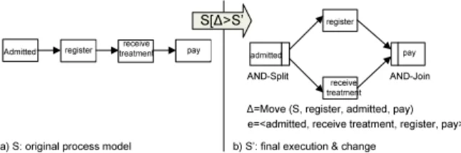
In response to this need adaptive process management technology has emerged [29]. It allows to adapt and configure process models at different levels. This, in turn, results in large collections of process model variants (process variants for short), which are created from the same process model, but slightly differ from each other in their structure. Fig. 1 depicts an example. The left hand side shows a high-level view on a patient treatment process as it is normally executed: a pa- tient isadmittedto a hospital, where he firstregisters, thenreceives treatment, and finally pays. In emergency situations, however, it might become necessary to deviate from this model, e.g., by first starting treatment of the patient and allowing him to register later during treatment. To capture this behavior in the model of the corresponding process instance, we need to move activityreceive treatment from its current position to a position parallel to activity register.
This leads to an instance-specific process model variantS0 as shown on the right hand side of Fig. 1. Generally, a large number of process variants may exist in a Process-Aware Information System (PAIS) at both the process type and process instance level [14].
S[∆>S’
receive treatment Admitted
a) S: original process model
register pay
b) S’: final execution & change register
receive treatment
pay
AND-Split AND-Join
admitted
∆=Move (S, register, admitted, pay) e=<admitted, receive treatment, register, pay>
Fig. 1.Original Process Model S and Process Variant S’
In most approaches which allow for the adaptation and configuration of pro- cess models, the resulting process variants have to be maintained separately.
Then even simple changes (e.g. due to new laws) often require manual re-editing of a large number of process variants. Over time this leads to divergence of the respective process models, which aggravates their maintenance significantly [31].
Considering a given reference process model and analyzing the collection of process variants configured from it, this paper aims at finding the problem mak- ers, i.e., the activities that are involved in process adaptations more often than others. These activities, in turn, cause most deviations from the reference process model and thus lead to highest configuration effort. In particular, we provide al- gorithms that solely use the reference process model and a collection of variants derived from it as input; i.e., we do not require the presence of a change log [18,
19] The discovered information is particularly useful for monitoring the devia- tions from the predefined process model or for redesigning it through learning from past executions.
Based on the two assumptions that: (1) process models are block-structured [17] (like for example BPEL 4) and (2) all activities in a process model have unique labels, this paper deals with the following fundamental research ques- tion:Given a reference process model and a collection of process variants config- ured from it, how to rank the activities according to their involvement in struc- tural process adaptations (i.e., the adaptations that become necessary when con- figuring the process variants)?
The remainder of this paper is organized as follows: Section 2 gives back- ground information needed for understanding this paper. To illustrate our algo- rithms, we provide an running example in Section 3. We provide a precise, but expensive ranking algorithm in Section 4 and a more efficient approximation ranking algorithm in Section 5. To test the performance of the two algorithms, we conduct comprehensive simulation. Section 6 describes the setup of this sim- ulation whereas Section 7 presents its result. Finally, Section 8 discusses related work and Section 9 concludes with a summary and an outlook.
2 Backgrounds
We first introduce basic notions needed in the following:
Process Model: Let P denote the set of all sound process models. A par- ticular process model S = (N, E, . . .)∈ P is defined as well-structured Activity Net [17, 29].N constitutes the set of process activities andE the set of control edges (i.e., precedence relations) linking them. To limit the scope, we assume Activity Nets to be block-structured like in BPEL. An example is provided in Fig. 1.
Process changeA process change is accomplished by applying a sequence of change operations to the process modelS over time [17]. Such change operations modify the initial process model by altering the set of activities and their order relations. Thus, each application of a change operation results in a new process model. We define process change andprocess variant as follows:
Definition 1 (Process Change and Process Variant). Let P denote the set of possible process models and C be the set of possible process changes. Let S, S0 ∈ P be two process models, let ∆ ∈ C be a process change expressed in terms of a high-level change operation, and let σ =h∆1, ∆2, . . . ∆ni ∈ C∗ be a sequence of process changes performed on initial model S. Then:
– S[∆iS0 iff∆is applicable toS andS0 is the (sound) process model resulting from the application of∆ toS.
– S[σiS0 iff ∃ S1, S2, . . . Sn+1 ∈ P with S = S1, S0 =Sn+1, and Si[∆iiSi+1
fori∈ {1, . . . n}. We denote S0 as variant of S.
4 see [28] for a technique transforming an unstructured process a model to block (tree) structured model
Examples of high-level change operations includeinsert activity, delete ac- tivity, andmove activity as implemented in the ADEPT change framework [17].
Whileinsert anddelete modify the set of activities in the process model,move changes activity positions and thus the order relations of the process model. For example, operation move(S,A,B,C) moves activity A from its current position within process model S to the position after activity B and before activity C.
Operationdelete(S, A), in turn, deletes activityAfrom process modelS. Issues concerning the correct use of these operations, their generalizations, and formal pre-/post-conditions are described in [17]. Though the depicted change oper- ations are discussed in relation to our ADEPT approach, they are generic in the sense that they can be easily applied in connection with other process meta models as well [29]. For example, a process change as described in the ADEPT framework can be mapped to the concept of life-cycle inheritance known from Petri Nets [25]. We refer to ADEPT since it covers by far most high-level change patterns and change support features when compared to other approaches [29], and it offers a fully implemented adaptive process engine.
Definition 2 (Distance and Bias). Let S, S0 ∈ P be two process models.
Then: Distance d(S,S0) between S and S0 corresponds to the minimal number of high-level change operations needed to transform process modelS into process modelS0; i.e.,d(S,S0):=min{|σ| |σ∈ C∗∧S[σiS0}. Furthermore, a sequence of change operationsσwithS[σiS0and|σ|=d(S,S0)is denoted as abiasbetweenS andS0. All the biases are summarized in a setB(S,S0)={σ∈ C∗| |σ|=dS,S0}, which we denote this set as the bias set.
Thedistance between two process models S and S0 is the minimal number of high-level change operations needed for transforming S into S0. Usually, it measures the complexity for model transformation. The corresponding sequence of change operations is denoted asbiasbetweenSandS0. Generally, it is possible to have more than one minimal sequence of change operations to realize the transformation from S into S0, i.e., given two process models S and S0 their bias is not necessarily unique [26, 12]. As example consider Fig. 1. Here, the distance between model S and process variantS0 isone, since we only need to perform one change operation ∆1 = move(S,register, addmitted, pay) to transformSintoS1. However, it is also possible to transformSintoS0with∆2= move(S,receive treatment, admitted, pay). Therefore, we obtainB(S,S0)= {∆1, ∆2}as bias set. In general, determining the bias and distance between two process models has complexity atN P level (see [12] for a computation method).
Here, we use high-level change operations rather than change primitives (i.e.
elementary changes like adding or removing nodes and edges) to measure the distance between process models. This allows to guarantee soundness of process models and also provides a more meaningful measure for distance [12].
Trace: A trace t on process model S = (N, E, . . .) denotes a valid and complete execution sequencet≡< a1, a2, . . . , ak>of activitiesai∈N according to the control flow set out by S. All traces S can produce are summarized in trace set TS. t(a ≺ b) is denoted as precedence relation between activities a
and b in trace t ≡< a1, a2, . . . , ak > iff ∃i < j : ai = a∧aj = b. Here, we only consider traces composing ’real’ activities, but no events related to silent ones (i.e. activity nodes which contain no action and exist only for control flow purpose [12]). Finally, we consider two process models being the same if they are trace equivalent, i.e.,S≡S0iffTS ≡ TS0. The stronger notion of bi-similarity [8]
is not required here.
3 Running Example
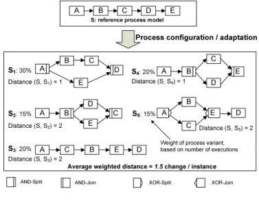
Fig. 2 gives an example, which is used for illustration purpose through out this paper. Regarding this example, out of a reference modelS, five different process variantsSi ∈ P (i= 1,2, . . .5) have been configured, which are weighted based on the number of process instances created from them. In our example, 30%
of all process instances were executed according to process variant S1, while 15% of the instances ran on S2. If we only know process variants, but have no runtime information about related instance executions, we assume the variants to be equally weighted; i.e., every process variant then has weight 1/n, wheren corresponds to the number of given variants.
Process configuration / adaptation S1: 30%
S2: 15%
S3: 20%
S4: 20%
S5: 15%
B C
E
A D
D
A C B E
A
D E
B C
B E
A
C
D
A E
B
C
D
Weight of process variant, based on number of executions
Distance (S, S1) = 1
Distance (S, S2) = 2
Distance (S, S3) = 2
Distance (S, S4) = 1
Distance (S, S5) = 2
Average weighted distance = 1.5 change / instance
A B C D E
S: reference process model
AND-Split AND-Join XOR-Split XOR-Join
Fig. 2.One illustrative example
We first compute the distances (cf. Def. 2) between process modelS and its variants. For example, when comparingS withS1 we obtain distance one, i.e., we only need to perform one change operation (i.e. move(S,E,A,D)) to trans- form S into S1. Or when comparingS with S2, needed change operations are move(S,D,B,C) and move(S,E,B,C), and distance between S and S2 is two.
Based on the weight of each variant, we can compute theaverage weighted dis- tance between reference model S and its variants; e.g., the distances between
S and Si, and the weights are depicted in Fig. 2. As average weighted distance we obtain 1×0.3 + 2×0.15 + 2×0.2 + 1×0.2 + 2×0.15 = 1.5. This means we need to perform on average 1.5 change operations to transform the reference model to a process variant and corresponding instance respectively. Generally, the average weighted distance between a reference model and its process variants expresses how ”close” they are; i.e., the higher the average weighted distance is, the greater configuration efforts have become
Though we are able to compute the distances between the reference model and each variant, it is not clear which activities are most involved in these configurations. Clearly, we should focus on the activities which are more often involved in these configurations, as they cause the major effort with respect to process configuration. In this context, we need an approach for ranking the activities based on their involvement in process variants configurations. Since we do not presume any run-time data (like change logs [19], or execution logs [27]), it is not possible to know which activities have been involved in process configurations particularly. In the following section, we will provide a method to measure the potential involvement of each activityai in process configurations, which we denote as change impact i.e., CI(ai). And based on the change impact of each activity, we are able to rank the activities, lets denote such ranking aschange impact ranking list.
In this paper, we are interested in detecting changes of order relations in pro- cess models. Therefore, we only considermoveoperations but factor outinsert or deleteoperations. Note that the latter can be easily detected by comparing activity sets of two process models (for details, see [10, 12]).
4 Computing the Precise Change Impact Ranking List
Since we do not presume the presence of a change log or execution log respec- tively, the major information we can use for our analysis are the bias setBS,Si
which describe the structural differences between the reference process model and each of its variant Si. From the bias set, we are able to compute the mini- mal number of change operations needed to transform the reference modelSinto a particular variant Si. The bias set, therefore, can be considered as a purified change log for our analysis. In this section, we present a method to compute the change impact of each activity based on the bias sets. A general description of our approach is as follows:
1. We compute the bias sets BS,Si which describe the structural difference be- tween the reference modelS and all the variantsSi (cf. Section 4.1).
2. For each bias set BS,Si, we measure the involvement of each activity ai in the captured adaptation. (cf. Section 4.2).
3. The change impactCI(ai) of an activityai is then measured by its involve- ment in all bias setsBS,Si (cf. Section 4.2).
4.1 Computing Biases
Let us re-consider the example from Fig. 2. By scanning the reference process model S and a process variant Si(i= 1. . .5), we are able to compute bias set BS,Si [12]. This bias set contains all possible sequences of change operations transforming S into Si with minimal number of change operations. However, the definition of bias set is too strict in our context, since we are only interested in the activities being involved in adaptation rather than the order in which the different changes were applied. For example, the bias set B(S,S2) comprise the two changes σ1, σ2 where σ1 =< ∆1, ∆2 > with ∆1 = move(S,D, B, C) and
∆2=move(S,E, B, C) andσ2=< ∆2, ∆1>. Althoughσ16=σ2, this difference is not relevant in our context since we are only interested in the activities being changed rather than the order in which different changes were applied.
Therefore, we keep the granularity of our bias analysis only on the activities that have been involved in changes changed rather than the applied change operations. Regarding our example, we only want to document these activities i.e.,{D,E} in the context ofσ1 (see above) rather than the change operationσ1
itself. When only looking at the changed activities, σ1 does not differ from σ2
since the activities concerned by the changes in the two biases are exactly the same.
Definition 3 (Changed Activity Set).
We define setAσrepresenting the activities changed by any change operation of biasσ, i.e.,Aσ={ai|(aiis an activity changed by ∆i)∧(∆i ∈σ)}. We define C(S,S0)={Aσ|σ∈ B(S,S0)} as theChanged Activity Setof S andS0.
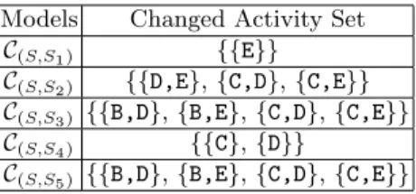
According to Def. 3, an element Aσ of the Changed Activity Set C(S,S0) corresponds to a set representing the activities changed by bias σ. Regarding our example from Fig. 2, the changed activity sets of the reference modelS and its variants Si (i= 1. . .5) are listed in Table 1.
Models Changed Activity Set C(S,S1) {{E}}
C(S,S2) {{D,E},{C,D},{C,E}}
C(S,S3) {{B,D},{B,E},{C,D},{C,E}}
C(S,S4) {{C},{D}}
C(S,S5) {{B,D},{B,E},{C,D},{C,E}}
Table 1.the Changed activity sets between reference model and all variants
As example, considerC(S,S2). We can either move activitiesDandE, or activ- itiesCand Dor activitiesC andEto transform modelS intoS2. When further analyzing Table 1, we can see thatC(S,S3)is exactly the same asC(S,S5)though the two process models S3 and S5 are quite different (cf. Fig. 2). The reason behind is that, for example, regarding move operations, the Changed Activity
Set only documents which activity has potentially been changed but does not specify to which position the activity have been moved to. Consequently, bias sets B(S,S3) and B(S,S5), which document the complete information about the changes, are rather different. However, in connection with the research ques- tion described in Section 1, we are only interested in activities which have been potentially involved in a change.
4.2 Computing the Change Impact CI(ai) of Each Activity ai
We measure the change impact CI(ai) of each activity ai by computing its contribution to the average weighted distance between the reference model and its variants. As example, consider distance d(S,S2) between reference model S and variant S2, which is 2. Here we want to measure how much each activity has contributed to this distance. We measure it by analyzing changed activity setCS,S2.
In general, for a given changed activity set, we enumerate all possible so- lutions to transform the reference process model S into the variants Si, i.e.,
∀Aσ ∈ C(S,Si): ∃σ ∈ B(S,Si). Note that we do not have any information about which sequence of change operations was applied to configureSiout ofS. There- fore, to each Aσ ∈ CS,Si we assign same weight d(S,Si)/|CS,Si|. Finally, for a particular activity aj ∈ Aσ∈ CS,Si, we choose |Cd(S,Si)
(S,Si)|×|A1
σ|.
Consider again the definition for the distance between process modelsS and Si(cf. Def. 2). Thend(S,Si)=|Aσ|holds, since biasσis a sequence with minimal number of change operations to transform S into Si. Consequently, the change impact for each activity aj between S and a particular Si can be computed as
|{Aσ∈C(S,Si)|aj∈Aσ}|
|C(S,Si)| .
LetS be the reference model and let Si(i = 1, . . . , n) be weighted process variantsSi(with weightwiandΣ1nwi= 1) derived fromS. Then the Change Im- pactCI(aj) of a particular activityaj, which measures its potential involvement in process adaptations, can be computed as follows:
CI(aj) = Xn i=1
wi×|{Aσ∈ C(S,Si)|aj∈ Aσ}|
|C(S,Si)| (1)
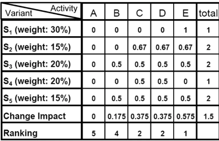
Figure 3 summarizes the Change Impacts of the activities from our example (cf. Figure 2). When reading the depicted table horizontally, it shows the poten- tial involvement of each activity when configuring the reference model S into a particular variantSi. As example takeS4. The distance betweenSandS4is one, since both activitiesCandDcould be potentially involved in the corresponding configuration (cf. Table 1). Each of the two activities therefore obtain Change Impact of 0.5 from this particular variant. When reading Figure 3 vertically, it shows the Change Impact of each activity based on the observation of all vari- ants. For example, activityBshows Change Impact of 0.5 for configuring variant S3and 0.5 for configuring variantS5. Considering the weight of each variant, the change impact of activity B CI(B) can be computed by Formula (1). As result
we obtain 0.175, which means that on average we need to move activityB0.175 times when configuring a variant out of the given reference model.
Activity Variant
Fig. 3.The change impact for each activity
Based on the change impact of each activity, we can also rank them accord- ingly. Clearly, activityEhas the highest change impact and therefore should be ranked first. Consequently, if we need to find an activity of the reference process model for re-positioning, activityEwill be the first candidate. Reason is that it has been reconfigured (i.e., re-positioned) more often than the other activities.
In fact, we have determined the contribution each activity has on the average weighted distance between the reference model and its variants. If we sum up the change impact of all activities, we obtain 0 + 0.175 + 0.375 + 0.375 + 0.575
= 1.5. Note that this corresponds to the actual value of the average weighted distance (cf. Fig. 2).
4.3 Discussion
The approach we described in this section is very precise: all possible changes be- tween the reference model and a process variant are enumerated and the change impact of a particular activity is computed by analyzing the reference model and all variants. However, enumerating all possible changes between two models is aN P problem, this approach can be very expensive. We need to call theN P algorithm every time we want to find possible changes between the reference model and a particular variant. Therefore, this approach will not scale up. If we have to deal with a large number of variants with complex structures (like models with tens up to hundreds of activities). In the next section, we introduce an approximation algorithm to solve the problem in an efficient way.
5 Compute the Approximation Change Impact Ranking List
To reduce the complexity for computing the change impact of each activity, we now introduce an approximation algorithm which only requires polynomial time to compute the ranking result. We first introduce the notion of order matrix in Section 5.1 and the notion of aggregated order matrix in Section 5.2. Section 5.3 then presents our approximation ranking algorithm.
5.1 Representing Process Models as Order Matrices
Theoretical backgrounds of high-level change operations have been extensively discussed in ADEPT [17]. One key feature of our ADEPT change framework is to maintain the structure of the unchanged parts of a process model [17].
For example, when deleting an activity this neither influences the successors nor predecessors of this activity, and therefore also not their order relations.
To incorporate this feature in our approach, rather than only looking at di- rect predecessor-successor relationships between activities (i.e. control edges), we consider the transitive control dependencies for each activity pairs; i.e. for a given process modelS= (N, E, . . .)∈ P, we examine for every pair of activities ai, aj∈N,ai6=ajtheir transitive order relations. Logically, we determine order relations by considering all traces the process model may produce (cf. Section 2).
Results are aggregated in an order matrixA|N|×|N|, which considers four types of control relations (cf. Def. 4):
Definition 4 (Order matrix). Let S = (N, E, . . .) ∈ P be a process model with N ={a1, a2, . . . , an}. Let furtherTS denote the set of all traces producible onS. Then: MatrixA|N|×|N| is calledorder matrixofS withAij representing the order relation between activitiesai,aj ∈N,i6=j iff:
– Aij = ’1’ iff (∀t∈ TS with ai, aj∈t⇒t(ai ≺aj))
If for all traces containing activitiesai andaj,ai always appears BEFORE aj, we denoteAij as ’1’, i.e.,ai always precedes ofaj in the flow of control.
– Aij = ’0’ iff (∀t∈ TS with ai, aj∈t⇒t(aj ≺ai))
If for all traces containing activities ai andaj, ai always appears AFTER aj, we denoteAij as a ’0’, i.e.ai always succeeds ofajin the flow of control.
– Aij = ’*’ iff (∃t1 ∈ TS, with ai, aj ∈ t1∧t1(ai ≺ aj)) ∧ (∃t2 ∈ TS, with ai, aj∈t2∧t2(aj≺ai))
If there exists at least one trace in which ai appears before aj and another trace in which ai appears afteraj, we denote Aij as ’*’, i.e. ai and aj are contained in different parallel branches.
– Aij = ’-’ iff (¬∃t∈ TS :ai∈t∧aj ∈t)
If there is no trace containing both activityai andaj, we denote Aij as ’-’, i.e.ai andaj are contained in different branches of a conditional branching.
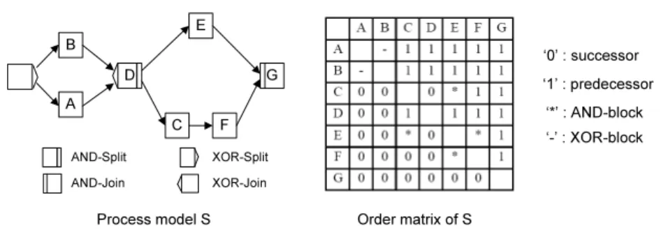
Fig. 4 shows an example. Besides control edges, which express direct predecessor- successor relationships, process modelSalso contains four kinds of control con- nectors: AND-Split and AND-Join (corresponding to a flow activity in BPEL),
A C
B E
F G D
Process model S Order matrix of S
AND-Split AND-Join
XOR-Split XOR-Join
‘0’ : successor
‘1’ : predecessor
‘*’ : AND-block
‘-’ : XOR-block
Fig. 4.Process model and its order matrix
and XOR-Split and XOR-join (corresponding to a switch or pick activity in BPEL). The depicted order matrix represents all four described relations. For example activitiesAandBwill never appear in the same trace since they are con- tained in different branches of an XOR block. Therefore, we assign ’-’ to matrix element AAB. Similarly, we can obtain the relation for each pair of activities.
The main diagonal of the matrix is empty since we do not compare an activity with itself.
Under certain conditions, an order matrix uniquely represents the process model it was created from. This is stated by Theorem 1. Before giving this theorem, we need to define the notion ofsubstring of trace:
Definition 5 (Substring of trace). Let S ∈ P be a process model and let t, t0 ∈ TS be two traces on S. We denote t as sub-string of t0 iff [∀ai, aj ∈ t, t(ai≺aj)⇒ ai,aj ∈t0∧t0(ai≺aj)] and [∃ak ∈N:ak ∈/ t∧ak∈t0].
Theorem 1. Let S, S0 ∈ P be two process models with same activity set N = {a1, a2, . . . , an}. Let furtherTS,TS0 be the related trace sets andAn×n,A0n×n be the order matrices of S andS0. ThenS6=S0 ⇔A6=A0, if [¬∃t1, t01∈ TS:t1 is a substring oft01] and [¬∃t2, t02∈ TS0:t2 is a substring oft02].
We give a proof of Theorem 1 in [12]. According to this theorem, there will be a one-to-one mapping between a process modelS and its order matrix A, if the substring constraint is met. (Note that the substring constraint can be easily checked and handled [12]); i.e., if the conditions of Theorem 1 are met, the order matrix will uniquely represent the process model. Analyzing its order matrix (cf.
Def. 4) will then be sufficient in order to analyze the process model.
5.2 Aggregated Order Matrix
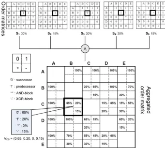
In order to analyze a given collection of process variants, we first compute the order matrix for each of these process variants (cf. Def. 4). Regarding our example from Fig. 2, for instance we obtain five order matrices (cf. Fig. 5). Then, we analyze the order relation for each pair of activities considering all five order matrices derived before. As the order relation between two activities might be not
the same in all order matrices, this analysis does not result in a fixed relationship, but provides a distribution for the four types of order relations (cf. Def. 4).
Regarding our example, in 65% of all cases activityC is a successor of activity B(as for variants S1, S2, S4), in 20% of all casesC is a predecessor of B (as in S3), and in 15% of the cases,Band Care contained in different branches of an XOR block (as in S5) (cf. Fig. 5). Therefore, we can define the order relation between two activitiesaandbas 4-dimensional vectorVab= (vab0 , v1ab, vab∗ , vab−):
each field corresponds to the frequency of the corresponding relation type (’0’,
’1’, ’*’ or ’-’) as specified in Def. 4. Take our example from Fig. 5: herev1CB= 0.65 corresponds to the frequency of all cases with activities B and C having order relation ’1’, i.e. all cases for which C precedes B. Regarding our example, we obtainVCB = (0.65,0.2,0,0.15).
We define anaggregated order matrix as follows:
Definition 6 (Aggregated Order Matrix).
LetSi∈ P,i= 1,2, . . . , nbe a collection of process variants with same activ- ity set N. Let furtherAi be the order matrix ofSi, and let weightwi represent the relative frequency of process instances executed on basis of Si. TheAggre- gated Order Matrixof all process variants is defined as 2-dimensional matrix Vm×m with m =|N| and each matrix element vjk = (vjk0 , vjk1 , v∗jk, v−jk)being a 4-dimensional vector. Forτ∈ {0,1,∗,−}, elementvτjkexpresses to what percent- age, activities aj and ak have order relation τ within the collection of process variantsSi. Formally:
∀aj, ak∈N, aj6=ak,∀τ∈ {0,1,∗,−} :vτjk = (Pn
i=1,Aijk=0τ0wi)/(Pn
i=1wi).
0 1
* -
‘0’ : successor
‘1’ : predecessor
‘*’ : AND-block
‘-’ : XOR-block
S1: 30% S2: 15% S3: 20% S4: 20% S5: 15%
V
VCB= (0.65, 0.20, 0, 0.15)
‘0’ : 65%
‘1’ : 20%
‘*’ : 0%
‘-’ : 15%
Order matrices Aggregatedorder matrix
Fig. 5.Aggregated order matrixV
Fig. 5 shows the aggregated order matrix of the process variants from Fig.
2. In an aggregated order matrix, main diagonal is always empty since we do not specify the order relation of an activity with itself. For all other elements, a non-filled value in a certain dimension means it corresponds to zero.
5.3 Approximation Algorithm for Ranking Activities According to Their Change Impact
We have introduced the aggregated order matrix to reflect the fact that the execution orders between two activities may not be the same in different variants.
For example, the execution orders between activitiesCandBcan be represented by VCB = (0.65,0.2,0,0.15). When reconsidering the reference process model from Fig. 2, we can see that the order relation between activities C and B is
”0”, i.e., C is a successor of B. If we built an aggregated order matrix Vref purely based on this reference model, as relationship betweenCandBwe would obtain VCBref = (1,0,0,0), i.e.,C would then always be a successor of B. When comparing VCB = (0.65,0.2,0,0.15) (which represents the variants) and VCBref (which represents the reference model), we can easily see that these two vectors are not the same. This indicates that when configuring reference model into the variants, the position of BorCmight have changed afterwards.
Configuring the reference model into a variant is realized by applying a se- quence of change operations (cf. Def. 1). Such an operation either changes the activity set (like insert and delete operations) or the original relationship be- tween the activities (e.g.move operation) of the reference model. Interestingly, the changes of the activity relations are represented by the changes of the order matrix. When configuring the reference model into variantS1, for example, we need to move activityEto the position betweenAandD, (i.e.,move(S,E, A, D)).
This change influences the order relation of E with the other activities. In the reference modelS for example,EsucceedsA, C, andD. Regarding process vari- ant S1 configured out of it by applying a move operation, the order relations betweenE on the one side andB, C and Don the other side is changed, i.e.,E now precedesDand is allocated in parallel toBandC.
Generally, we can assume that the more an activity is moved, the more its order relation differs from the original one. To quantitatively measure this difference, we compare the order relations set out by the reference model with those of the aggregated order matrix.
Before providing the comparison method, we first introduce functionf(α, β) which expresses the closeness between two vectors α= (x1, x2, ..., xn) and β = (y1, y2, ..., yn):
f(α, β) = α·β
|α| × |β| =
Pn
i=1xiyi
pPn
i=1x2i ×pPn
i=1yi2 (2)
f(α, β)∈[0,1] computes the cosine value of the angle θ between vectors α and β in Euclidean space. Iff(α, β) = 1 holds,αandβ exactly match in their directions;f(α, β) = 0 means, they do not match at all. Regarding our running
examples, for instance, we obtainf(VCB, VCBref) = 0.933. This number indicates high similarity between the order relations of the reference model and the ones of the variants (which are represented by the aggregated order matrix).
Based on these considerations, the change impact of a particular activity can be measured using the following formula. To differentiate it from Formula (1), we denote change impact computed by this approximation asCIa(ai).
CIa(ai)5= P
x∈N\{ai}f2(Vaix, Varefix)
|N| −1 (3)
CIa(ai)∈[0,1] corresponds to the average square mean value of the similarity (measured by Formula (2)) between activityaiand the rest of activities. It there- fore approximately reflects how muchai has been re-configured. If CIa(ai) = 1 holds, activityaiwill exactly have same order relations with respect to the other activities in both the reference model and all the variants. For this case, We can therefore assume that it has not been moved.W eight(ai) = 0, in turn, means that the order relation of ai as reflected shown in the reference model is com- pletely different from the order relations in the different variants. We therefore assume that in such case activityaihas been moved a lot. Note that our ranking is based on descending orders, i.e., the higher the change impactCIa(ai) is, the lower the chance will be that it has been potentially moved and the lower such activity should be ranked.
Regarding our example from Fig. 2, the ranking result of the five activities is shown in Table 2.
Activity E D C B A
CIa(ai) 0.6641 0.7384 0.8678 0.9280 1.0000
Rank 1 2 3 4 5
Table 2.Approximate ranking result
From Table 2, we can clearly derive a ranking order of the activities based on their potential involvement in changes. ActivityE is moved most frequently while activity Ais the least moved one.
5 Note that this is not a precise measure since not only the execution orders of the moved activities are affected, but the other activities may be influenced by a change operation as well. For example, when configuringSintoS1, we actually only need to move activityE. However, the execution orders of the remaining activities are also changed, e.g., activities B, C and D. Reason is that move operations can globally influence the execution order while our measure only examines the local information between every pair of activities.
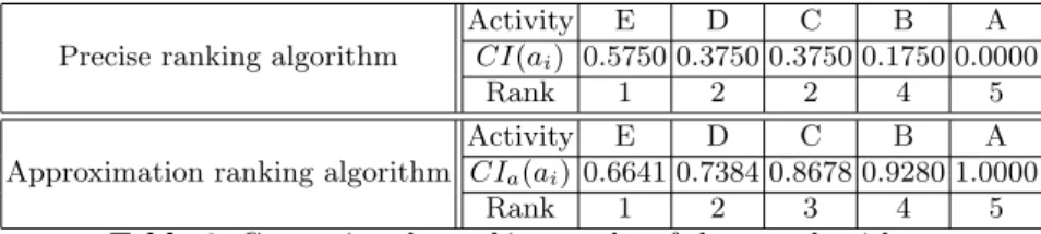
5.4 Comparing the Precision ranking Algorithm and the Approximation Ranking Algorithm
The approximation algorithm presented in Section 5.3 is a polynomial algorithm, i.e., the complexity for computing the change impactCIa(ai) of activityaivalue of an activity is atO(n2×m) wherenis the number of activities in each variant andmis the number of variants.6 Compared to theN P level complexity of the precise ranking algorithm, efficiency of the approximation ranking algorithm is much better. However, we still have to validate the performance of the approx- imation algorithm, i.e., we must show how close it is to the real optimum (i.e., the ranking provided by the precise ranking algorithm). Regarding our running example, comparison results are summarized in Table 3.
Precise ranking algorithm
Activity E D C B A
CI(ai) 0.5750 0.3750 0.3750 0.1750 0.0000
Rank 1 2 2 4 5
Approximation ranking algorithm
Activity E D C B A
CIa(ai) 0.6641 0.7384 0.8678 0.9280 1.0000
Rank 1 2 3 4 5
Table 3.Comparing the ranking results of the two algorithms
Table 3 shows the ranking results for our example from Fig. 2 using both precise ranking algorithm and the approximation ranking algorithm. More pre- cisely, tt shows the change impact of each activity, as well as its ranking order.
This simple comparison already indicate that that the performance of the ap- proximation ranking algorithm is quite good. Here, it generates the same ranking order as the precise ranking algorithm does.
Of course, such a simple comparison is far from being sufficient. First, as the comparison is only based on one example, it is not allowed to draw general conclusion about the performance of the approximation algorithm. Clearly, it cannotNOT perfectly match the precise ranking algorithm, since the latter one hasN P level complexity. While the approximation ranking algorithm only tries to achieve an approximation using a polynomial algorithm. A more systematic comparison is required to evaluate the real performance of the approximation ranking algorithm. In this context, we are also interested in those factors that influence the performance of the approximation ranking algorithm. In the fol- lowing, we try to answer the following two questions:
6 The complexity is computed based on the assumption that we have already had the order matrices for the reference model and the variants. Since the complexity for computing the order matrix from a process model is atO(n2), the overall complexity for computing the ranking value of an activity isO(m×n2+n) wherenis the number of activities andmis the number of variants.
1. How good does the approximation algorithm perform, i.e., how close are its ranking results in comparison to the precise ranking results?
2. What factors have influence on the performance of the approximation ranking algorithm, i.e., based on what conditions does it perform better or worse?
6 Simulation
We use simulation to answer the above questions, i.e., by generating hundreds or thousands of examples, we are able to conclude statistically how good the performance of the algorithm is and to test which factors significantly influence it.
In order to analyze the influential factors, we require the dataset for simula- tion to be well structured and well understood, i.e., we need to know the features of the dataset which we are analyzing in order to determine which parameters are more important than others. So far, there are no such real-life data available for simulation. And even if this had been the case, such data would certainly not cover all the scenarios we want to examine. Therefore, we use automatically created datasets to run our simulations.
This section will describe how the dataset are generated. Since both the ranking algorithms require a reference process model and a collections of process variants derived from it, this section has been divided into three subsections:
1. We first describe an algorithm to randomly generate a reference model in Section 6.1.
2. Besides purely examining the performance of our algorithms, we are also interested in whether the performance of our algorithms can be influenced by some external parameters (like the size of the models or the similarity between the models, etc). Therefore, Section 6.2 describes which parameters will be considered when configuring the reference model into process variants.
3. Section 6.3 then describes how we adjust the different parameters in config- uring the process variants.
In the following, we generate 36 groups of datasets using different values for the parameters we consider. For each of these groups, we generate 1 reference model and 100 process variants configured out of the reference model (i.e., we consider 3636 process models). For creating the data sets, we assume different scenarios. We compare the two ranking algorithms based on the ranking results we obtain from the 36 groups. In the following, we describe the scenarios we used to generate the datasets and in the next section (cf. Section 7), we will evaluated the ranking result of the different algorithms.
6.1 Generating the Reference Process Model
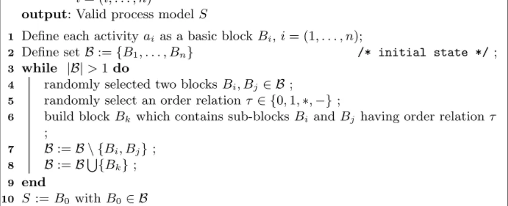
Our general idea of randomly generating (block structured) reference model is to cluster blocks, i.e., we randomly cluster activities (blocks) into a bigger block and
input : Set of activitiesaithe process model to be generated should contain, i= (i, . . . , n)
output: Valid process modelS
Define each activityaias a basic blockBi,i= (1, . . . , n);
1
Define setB:={B1, . . . , Bn} /* initial state */;
2
while |B|>1do
3
randomly selected two blocksBi, Bj∈ B;
4
randomly select an order relationτ ∈ {0,1,∗,−};
5
build blockBkwhich contains sub-blocksBiandBjhaving order relationτ
6
;
B:=B \ {Bi, Bj};
7
B:=BS {Bk};
8
end
9
S:=B0 withB0∈ B
10
Algorithm 1: Randomly generating a reference model
this clustering continues iteratively until all the activities (blocks) are clustered together. The detail of our approach is depicted in algorithm 1.
To illustrate how Algorithm 1 works, an example is given in Fig. 6. As input a set of activities{A,B,C,EandE}are given, and the goal is to construct a valid, block-structured process modelS out of them. The algorithm starts by consid- ering each activityai as basic blockBi, and adding these blocks to setB(lines 1 and 2). Regarding our example, B={{A},{B},{C},{D},{E}}. The algorithm first randomly select two blocksBi, Bj (lines 4) and link them with a randomly chosen order relationτ (lines 5 and 6). Regarding our example, blocks{B} and {C} are selected to construct a new block{B, C}with a randomly chosen order relation 1 (which meansBprecedesC). The newly created block{B, C}will then replace blocks {B} and {C} in the block setB, i.e., B ={{A},{B,C},{D},{E}}
(lines 7 and 8). This procedure (lines 4-8) is repeated until block setBcontains one single blockB0(B0={A,B,C,D,E}regarding our example). This block then represents our randomly generated process modelS. (line 10). Fig. 6 shows the process model we randomly generated as well as the block constructed in each iteration.
A
B C E D
1
*
1
Order relation 0
randomly chosen
Result
B C
E
D A
1 2
3 4
Fig. 6.Example of generating random process model
In practise, certain order relations are used more often than others. For exam- ple, the predecessor-successor relation is used more frequently than AND/XOR- splits [33]. When randomly generating a process model, we therefore take this into account as well. Rather than randomly setting the order relation for two blocks, we set the probability for choosing AND-split (τ =0 ∗0) and XOR- split (τ =0 −0) to 10% respectively, while predecessor-successor relationships (τ={0,1}) are chosen with probability of 80%.
We therefore randomly generate 3 reference models, containing 10, 20 and 50 activity respectively 7. According to [15], process models containing more than 50 activities have high risk of errors. therefore, it is not recommended to design such large model. Following this guideline, we also set the largest size of a process model for 50 activities in our simulation.
6.2 Parameters Considered for Generating Process Variants
Taking a generated reference process model, we control how variants are config- ured by adjusting specific parameters. For example, these parameters determine how many change operations needed to perform to configure a particular vari- ant and where activities should be moved to and so forth. Basically, we have considered the following parameters when generating the process variants.
1. Parameter 1 (Size of Process Models)The size of a variant (i.e., the number of its activities) can potentially influence results. Therefore, we need to check the behavior of our algorithm when applying them to variants of different sizes. This is also important to test the scalability of the approxi- mation algorithm, whose performance should not depend on the size of the sample data.
2. (Parameter 2 (Similarity of Process Variants) This parameter mea- sures how ”close” these variants are, e.g., whether or not the variants are similar to each other. In this context, similarity measures how difficult it is to configure one variant into another [12].
3. Parameter 3 (The Activities Been Changed) Often we can observe that the probability with which activities are changed is not uniformly dis- tributed, i.e., some activities might be involved in changes more often than others. We therefore want to analyze whether the probability distribution of how frequently an activity is changed would thus influence the performance of our algorithms.
4. Parameter 4 (Position Where Activities Are Moved To)Change can be local or global. A local change will influence the order relations of only very few activities (e.g., when swapping the order of two directly succeeding activities) while global ones can influence quite a lot of order relations in a process model (for example when moving one activity from the beginning to the end). Therefore, we need to check whether or not this influences the results.
7 Each of these model will be used in 12 groups of datasets, since we want to avoid the influence of the reference model. A detailed discussion can be found later in Section 6.3
6.3 Method for generating Data Sets
The dataset for our simulation analysis is generated by a randomly generating a reference model (cf. Section 6.1) and a collection of variants configured based on this reference model. When configuring these variants, by applying a sequences of change operations to the reference model, we vary the parameters described in Section 6.2 and consequently generate variants based on different scenarios.
The following choices are available for the different parameters:
Parameter 1 (Size of Process Models) This parameter controls how many activities shall be contained in a process model. There can be three options:
1. Small-sizedmodels : 10 activities per variant 2. Medium-sizedmodels: 20 activities per variant 3. Large-sizedmodels: 50 activities per variant
(Parameter 2 (Similarity of Process Variants)The closeness between the variants is measured by determining the total number of change operations we have to apply when generating variants (cf. Def. 2). Three possible choices exist:
1. Small change: 10% of activities are moved 2. Medium change: 20% of activities are moved 3. Large change: 30% of activities are moved
For example, for the datasets comprising large-size process variants (i.e., variants with 50 activities), medium-change would mean to randomly change 10 activities when generating generate a variant of the given a reference model. This way, we can control the distance between the reference model and its variant.
And indirectly, we can control the similarity between variants since they are all controlled in a certain distances with the reference model.
Parameter 3 (The Activities Been Changed)This parameter controls which activities are moved when generating the variant models. We consider two scenarios:
1. In this scenario, we randomly pick the activities be moved, i.e., each activity is assumed to have the same probability to be involved in a move operation.
As example assume that we need to move two activities in order to configure one particular variant out of the reference model. In this scenario, we assume each activity in the reference model would have the same probability to be chosen, i.e., we can randomly pick two different activities. Since every time activities are selected randomly, there will be no activity which has been moved significantly more often than others in the collection of variants.
Please note that it does not mean every activity will be changed exactly for the same number of times when configuring the collection of process variants.
Random differences will occur but these differences are not significant enough in a statistical sense. Table 4 shows one example for random picking activities with small model (10 activities) and small change (10% of them are changing, i.e., one change).
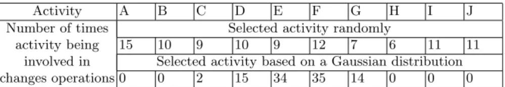
2. Activities are selected based on Gaussian distribution. Very often we can observe that some activities are involved in changes than others. We therefore have to simulate the situation in which activities are not been in- volved in change with same frequency. We set the probabilities for changing (i.e., moving) the activities by using a Gaussian distribution, i.e., some ac- tivities are assumed to be moved more often than others when generating the process variants. Ifncorresponds to the number of activities in the ref- erence model and we randomly give a permutation of the activity set: the probability for selection the numbernactivity follows Gaussian distribution X:(n/2,(n/10)2). This means the expected mean of the distribution isn/2 and its expected standard deviation is n/10. The Table 4 gives a general ideal of such distribution for a dataset with small size model (comprising 10 activities) and only small change (10% of them are changing) are performed to configure each process variant:
Activity A B C D E F G H I J
Number of times Selected activity randomly
activity being 15 10 9 10 9 12 7 6 11 11
involved in Selected activity based on a Gaussian distribution
changes operations 0 0 2 15 34 35 14 0 0 0
Table 4. When configuring 100 variants from the reference model, this table shows the number of times one particular activity being involved in change operations based on either random selection or Gaussian distribution
Parameter 4 (Position Where Activities Are Moved To). While pa- rameter 3 determines how frequent an activity is moved, Parameter 4 controls the position to which corresponding activities are moved to. Clearly, a local change (e.g., to swap the order of two directly succeeding activities) has less effects on order relations than a global change (e.g., move an activity from the beginning to the end). This section analyzes whether this will influence the performance of our ranking algorithms.
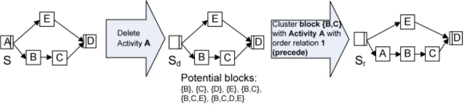
When performing a move operation, one important issue has to be considered.
Since we only consider block-structured process models, move operations must not ”destroy” this block structure. Given the reference modelSan the candidate activityai for moving, we perform the following three steps to guarantee block- structure of the resulting model:
1. We first remove activity aifrom the process modelS.
2. We enumerate all possible blocks the modified process model contains. A block can be one single activity or a self-contained part of the process model or even the model itself. (See Appendix A for an algorithm enumerating all possible blocks in a process model). Also note that the number of possible candidate blocks is normally very large, e.g., several hundred potential blocks can be identified for a large process model (with 50 activities).