An estimator for the quadratic covariation of asynchronously observed Itô processes with noise

SFB 649 Discussion Paper 2011-034

An estimator for the quadratic covariation of asynchronously

observed Itô processes with noise: Asymptotic distribution

theory

Markus Bibinger*

* Humboldt-Universität zu Berlin, Germany

This research was supported by the Deutsche

Forschungsgemeinschaft through the SFB 649 "Economic Risk".

http://sfb649.wiwi.hu-berlin.de ISSN 1860-5664

SFB 649, Humboldt-Universität zu Berlin Spandauer Straße 1, D-10178 Berlin

S FB

6 4 9

E C O N O M I C

R I S K

B E R L I N

An estimator for the quadratic covariation of asynchronously observed Itˆo processes with noise: Asymptotic distribution theory

Markus Bibinger¹

Institut f¨ur Mathematik, Humboldt-Universit¨at zu Berlin, Unter den Linden 6, 10099 Berlin, Germany

Abstract

The article is devoted to the nonparametric estimation of the quadratic covariation of non-synchronously observed Itˆo processes in an additive microstructure noise model. In a high-frequency setting, we aim at establishing an asymptotic distribution theory for a generalized multiscale estimator including a feasible central limit theorem with optimal convergence rate on convenient regularity assumptions. The inevitably remaining impact of asynchronous deterministic sampling schemes and noise corruption on the asymptotic distribution is precisely elucidated. A case study for various important examples, several generalizations of the model and an algorithm for the implementation warrant the utility of the estimation method in applications.

Keywords: non-synchronous observations, microstructure noise, integrated covolatility, multiscale estimator, stable limit theorem

MSC Classification:62M10, 62G05, 62G20, 91B84 JEL Classification:C14, C32, C58, G10

1. Introduction

The nonparametric estimation of the univariate quadratic variation of a latent semimartingale fromn observations in a high-frequency setting with additive observation noise has been studied intensively in recent years. It is known from [13] thatn^1/4 constitutes a lower bound for the rate of convergence. An important motivation which has stimulated an alliance of economists and statisticians to establish estima- tion techniques for this kind of latent semimartingale models is their utility in estimating daily integrated (co-)volatilities from high-frequency intraday returns that serve as a basis for risk management as well as portfolio optimization and hedging strategies. The last years have seen an enormous increase of the amount of trading activities for many liquid securities. Paradoxically, the availability of high-frequency data necessitated a new angle on financial modeling. In fact, for every semimartingale the discrete realized (co-)volatilities converge in probability to the integrated measures. However, realized volatilities of typical high-frequency financial time series data explode for very high frequencies. This effect is ascribed to mar- ket microstructure frictions. Sources of the market microstructure noise are manifold. One important role plays the occurrence of bid-ask spreads. Aside from that transaction costs, strategic trading, limited market depths and discreteness of prices spread out the structure of the long-run dynamics that can be character- ized by semimartingales.

This strand of literature followed [31] that has attracted a lot of attention to this estimation problem. The so-called two-scales realized volatility by [31] is based on subsampling and a bias-correction and a sta- ble central limit theorem withn^1/6-rate has been proved. A refinement of the subsample approach using multiple scales in [30] and related alternative techniques in [4], [23] and [29] have led to rate-optimal estimators and feasible stable central limit theorems. For the more specific nonparametric model with

1Financial support from the Deutsche Forschungsgemeinschaft via SFB 649 ‘ ¨Okonomisches Risiko’, Humboldt-Universit¨at zu Berlin, is gratefully acknowledged.

Gaussian noise, asymptotic equivalence in the Le Cam sense to a Gaussian shift experiment is shown in [26] and an asymptotically efficient estimator whose asymptotic variance equals the parametric efficiency bound is constructed.

In the article on hand we are concerned with a multivariate stetting and apart from taking additive mi- crostructure noise into account, we focus on a way to deal with non-synchronous observation schemes.

This is also a central theme in financial applications. When realized covolatilities are calculated for fixed time distances and a previous-tick interpolation is applied, the phenomenon of the so-called Epps effect described in [10] appears that the realized covolatility tends to zero at the highest frequencies.

A methodology to deal with non-synchronous observations in a bivariate Itˆo processes model has been proposed by [15]. The so-called Hayashi-Yoshida estimator has superseded simpler previous-tick inter- polation methods setting the standard for the estimation of the quadratic covariation from asynchronous observations in the absence of microstructure noise effects.

Our estimation approach, first proposed in [8], for the most general case in the presence of noise and non- synchronicity arises as a combination of the multiscale estimator to handle noise contamination on the one hand and a synchronization algorithm in accordance with the Hayashi-Yoshida estimator to cope with non- synchronicity on the other hand. A first attempt in the same direction, combining one-scale subsampling and the Hayashi-Yoshida estimator, has been given in [22].

In [8] it has been shown in the spirit of [13] that the optimal convergence raten^1/4carries over to the general multidimensional setup. The mathematical analysis of our generalized multiscale estimator in [8] shows that it is rate-optimal.

Alternative approaches to similar statistical models has been suggested by [5], [9] and [1]. In [5] a kernel- based method with a previous-tick interpolation to so-called refresh times is proposed and a stable central limit theorem with sub-optimaln^1/5-rate is established for a multivariate non-synchronous design. This estimator, furthermore, ensures that the estimated covariance matrix is positive semi-definite. [9] and [1]

come up with combinations of pre-averaging ([23],[19]) and the Hayashi-Yoshida estimator and of the univariate quasi-maximum-likelihood method by [29], the polarization identity and a generalized synchro- nization scheme which is different from the Hayashi-Yoshida ansatz that we use, respectively, both also attaining the optimal rate.

In this article we aim at providing an asymptotic distribution theory for the generalized multiscale estima- tor. In distinction from alternative methods, the influence of non-synchronicity effects on the expectation is null and on the variance limited up to an interaction of interpolation steps and microstructure noise. The main result is a feasible stable central limit theorem for its estimation error with optimal rate and a closed- form asymptotic variance that does not hinge on interpolation errors in the signal term. The stable weak convergence of the estimation error to a centred mixed Gaussian limit and the consistent estimation of the random unknown asymptotic variance are the essential steps towards statistical inference and confidence sets. The theory is grounded on stable limit theorems for semimartingales from [18].

In Section 2 we present the model and our main findings. Section 3 comes up with a concise overview on the construction of the estimator and in Section 4 we develop the asymptotic theory. In Section 5 we propose a consistent estimator for the asymptotic variance and Section 6 comprises various extensions and and a concluding discussion. The proofs are postponed to the Appendix.

2. Model and key result

The considered statistical model of noisy latently observed Itˆo processes at deterministic observation times is precisely described by Assumptions 1-3 in this section.

Assumption 1(efficient processes). On a filtered probability space(Ω,F,(Ft),P), the efficient processes X = (Xt)_t∈R+ and Y = (Yt)_t∈R+ are Itˆo processes defined by the following stochastic differential equations:

dX_t=µ^X_t dt+σ^X_t dB_t^X, dYt=µ^Y_t dt+σ^Y_t dB_t^Y ,

with two(F_t)–adapted standard Brownian motionsB^X andB^Y and ρ_tdt = d

B^X, B^Y

t. The drift processes µ^X_t and µ^Y_t are (F_t)–adapted locally bounded stochastic processes and the spot volatilities

σ^X_t andσ_t^Y andρtare assumed to be(Ft)–adapted with continuous paths. We assume strictly positive volatilities and the Novikov conditionE

h exp

(1/2)RT

0 (µ^·/σ^·)²_tdti

<∞forXandY.

Assumption 2(observations). The deterministic observation schemesT^X,n={0≤t⁽ⁿ⁾₀ < t⁽ⁿ⁾₁ < . . . <

t⁽ⁿ⁾n ≤T}ofX andT^Y,m ={0≤τ₀^(m)< τ₁^(m)< . . . < τm^(m)≤T}ofY are assumed to be regular in the following sense: There exists a constant0< α≤1/9such that

δ_n^X= sup

i∈{1,...,n}

t⁽ⁿ⁾_i −t⁽ⁿ⁾_i−1

, t⁽ⁿ⁾₀ , T −t⁽ⁿ⁾_n

=O

n^−8/9−α

, (1a)

δ^Y_m= sup

j∈{1,...,m}

τ_j^(m)−τ_j−1^(m)

, τ₀^(m), T −τ_m^(m)

=O

m^−8/9−α

. (1b)

We consider asymptotics where the number of observations ofX andY are assumed to be of the same asymptotic ordern=O(m)andm =O(n)and express that shortly byn∼m. The efficient processes X andY which satisfy Assumption 1 are discretely observed at the timesT^X,n andT^Y,mwith additive observation noise:

X˜_t(n) i

= Z t⁽ⁿ⁾_i

0

µ^X_t dt+ Z t⁽ⁿ⁾_i

0

σ_t^XdB^X_t +^X

t⁽ⁿ⁾_i ,0≤i≤n , (2a) Y˜_τ(m)

j

= Z τ_j^(m)

0

µ^Y_t dt+ Z τ_j^(m)

0

σ^Y_t dB_t^Y +^Y

τ_j^(m) ,0≤j≤m . (2b) Although we consider sequences of deterministic observation times, the case of random sampling that is independent of the observed processes is included when regarding the conditional law.

It turns out that it is accurate to prove the key result of the article on the following i. i. d. assumption on the microstructure noise since a closed-form expression for the asymptotic variance is not available for a combination of general asynchronous observation schemes and serially dependent observation errors.

Since an extension to non-i. i. d. noise is crucial for the utility in financial applications, we comment on the robustness of our estimator to that case in Section 6.

Assumption 3(microstructure noise). The discrete microstructure noise processes ^X

t⁽ⁿ⁾_i , ^Y

τ_j^(m),0≤i≤n,0≤j≤m .

are centred i. i. d. , independent of each other and independent of the efficient processesX and Y. We assume that the observation errors have finite fourth moments and denote the variances

η_X² =Var ^X

t⁽ⁿ⁾₁

, η²_Y =Var ^Y

τ₁^(m)

.

The number of synchronized observationsN ∼n∼mwhich appears in the rate of our feasible stable central limit theorem is introduced in Section 3.

Theorem 1(feasible stable central limit theorem). The generalized multiscale estimator(12)specified by the later given weights(A.1), withM_N =c_multi·√

Nconverges on the Assumptions 1, 2, 3 and further mild regularity conditions on the asymptotics of the sampling schemes, stated below in Assumptions 4 and 5,F −stably in law with optimal rateN^1/4∼n^1/4∼m^1/4to a mixed Gaussian limiting distribution:

N^1/4

[X, Y\]

multi

T −[X, Y]_T st

N(0,AVARmulti)

with an almost surely finite random asymptotic variance given in(18)in Theorem 3. With the consistent estimator for the asymptotic varianceAVAR\ _multiin Proposition 5.1 , the feasible central limit theorem

N^1/4

[X, Y\]

multi

T −[X, Y]_T

AVAR\ multi

st N(0,1), (3)

holds true.

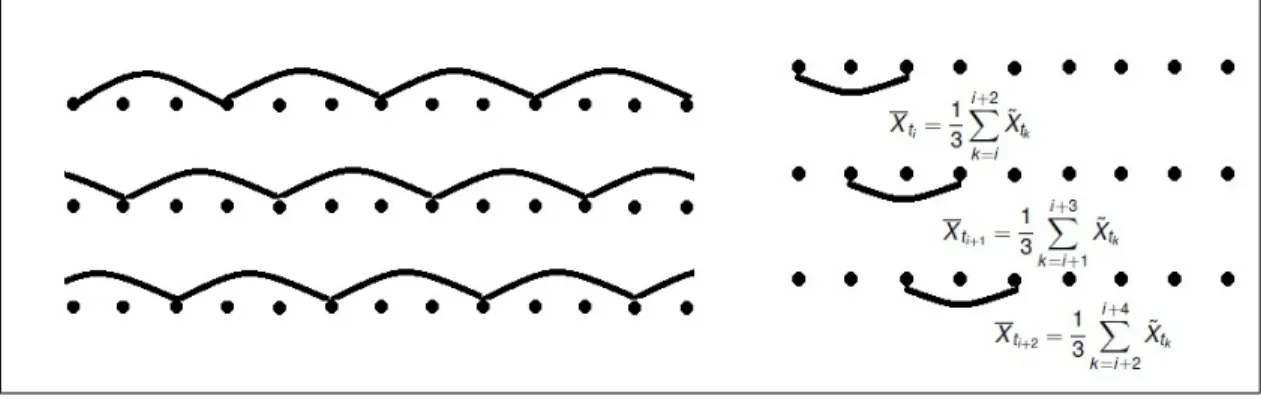
Figure 1: Sketch of the subsampling approach.

The notion of stable weak convergence going back to [27] is essential for our asymptotic theory. Stable weak convergenceX_n ^st X is the joint weak convergence of(X_n, Z)to(X, Z)for every measurable bounded random variableZ. The limiting random variables in stable limit theorems are defined on exten- sions of the original underlying probability spaces. The reason for us to involve this concept of a stronger mode of weak convergence is that mixed normal limiting distributions are derived where asymptotic vari- ances are themselves strictly positive random variables. Provided we have a consistent estimatorV_n²for such a random asymptotic varianceV²on hand, the stable central limit theoremXn

st V ZwithZ dis- tributed according to a standard Gaussian law, yields the joint weak convergence(Xn, V_n²) (V Z, V²) and alsoXn/Vn Zand hence allows to perform statistical inference providing tests or confidence inter- vals.

In the proofs of our limit theorems we will ‘remove’ the drifts in the sense that after a transformation to an equivalent martingale measure stable central limit theorems for Itˆo processes without drift are proved and, as illustrated in [21], stability of the weak convergence ensures that the asymptotic law holds true under the original measure. In this sense stable convergence is commutative with measure change.

From now on, we often omit the superscripts of observation times for a shorter notation.

3. Brief review on the foundation

3.1. Subsampling and the multiscale estimator

In the model imposed by Assumption 1, Assumption 2 with synchronous observations, n = mand t⁽ⁿ⁾_j =τ_j⁽ⁿ⁾,1≤j ≤n, and Assumption 3, the realized (co-)volatilities do not provide consistent estima- tors for the quadratic (co-)variations any more. The variance due to noise conditional on the paths of the efficient processes

VarX,Y





n

X

j=1

X˜_tj −X˜_tj−1 Y˜_tj −Y˜_tj−1



= 4n η_X²η²_Y ,

increases linearly withn. The error due to noise perturbation can be reduced by the following estimator, which has been proposed for the univariate estimation of integrated volatility as the “second best approach”

in [31] and which is called one-scale subsampling estimator in [8] and throughout this article. It can be motivated from two perspectives that are both sketched in Figure 1. On the left-hand side we have visualized that one can calculate simultaneously lower frequent realized covolatilities using subsamples, e. g. to the lag three in Figure 1, and (post-)average them.

[X, Y\]

sub T = 1

i

n

X

j=i

X˜t_j−X˜t_j−i Y˜t_j −Y˜t_j−i

. (4a)

This motivation given in [31] is in line with the former common practice of a sparse-sampled low-frequency realized (co-)volatility estimator and proposes to use an average instead of one single lower frequent real- ized measure.

The same estimator arises as the usual realized covolatility calculated from the time series on that a linear filter is run before, what means that non-noisy observations at a timetjare estimated with a (pre-)average of noisy observations at timestj, . . . , tj+ifor somei. This is sketched on the right-hand side of Figure 1 fori= 3. Passing over to increments leads to telescoping sums and we end up finally with the one-scale subsampling estimator.

Since on the Assumption 3 there is no bias due to noise for the bivariate estimator, it already corresponds to the “first best approach” from [31] whereas in the univariate case a bias-correction completes the two scales realized volatility (TSRV):

d[X]

T SRV

T = 1

i

n

X

j=i

X˜tj −X˜tj−i

²

− 1 2n

n

X

i=1

X˜tj −X˜tj−1

²

. (4b)

There is a trade-off between the signal term and the error due to noise. Choosingi=c_subn^2/3dependent on n with a constant c_sub, the overall mean square error is minimized and of order n^−1/3. The one- scale subsampling estimator (4a) is hence a consistent and asymptotically unbiased estimator. The rate of convergencen^1/6, however, is slow and does not attain the optimal rate n^1/4determined in [8]. For this reason, we focus on a multiscale extension of the subsampling approach on which the methods developed in [8] are based on. The multiscale realized covolatility (MSRC), and the univariate multiscale realized volatility (MSRV) introduced in [30], are linear combinations of one-scale subsampling estimators with Mndifferent subsampling frequenciesi= 1, . . . , Mn:

[X, Y\]

multi

T =

M_n

X

i=1

α^opt_i,M

n

i

n

X

j=i

X˜t_j−X˜t_j−i Y˜t_j −Y˜t_j−i

, (5a)

[X]d^multi_T =

M_n

X

i=1

α^opt_i,M

n

i

n

X

j=i

X˜t_j −X˜t_j−i

2

. (5b)

The weights are chosen such that the estimator is asymptotically unbiased and the error due to noise mini- mized. They are given later in (A.1) and can be chosen equally for the bivariate and the univariate case.

Those are the standard discrete weights of [30] and we abstain from giving a more general class of possible weight functions.

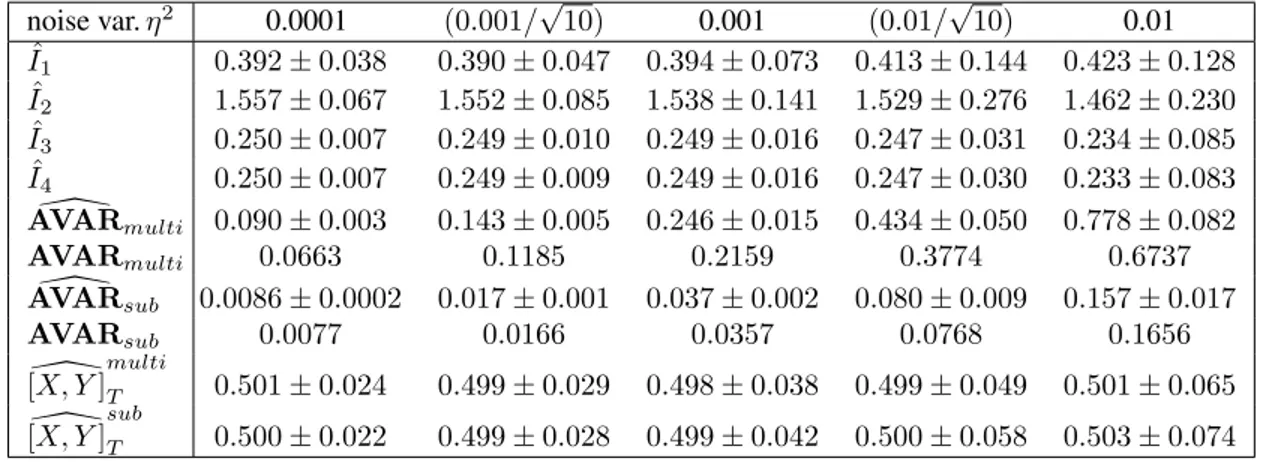
The mean square error of the multiscale realized covolatility (5a) can be split in uncorrelated addends that stem from discretization, microstructure noise and cross terms and end-effects. They are of ordersMn/n, n/M_n³, andM_n⁻¹, respectively. Hence, a choiceMn =cmulti

√nleads to a rate-optimaln^1/4-consistent estimator.

The following stable central limit theorems for the multiscale realized covolatility (5a) and the one-scale estimator (4a) are implied by Theorem 3 and Corollary 4.1:

Proposition 3.1. On Assumptions 1, 2 and 3 in the synchronous setup and if(n/T)P

i(t⁽ⁿ⁾_i −t⁽ⁿ⁾_i−1)²con- verges to a continuously differentiable limiting functionGand the difference quotients converge uniformly toG⁰on[0, T], the multiscale realized covolatility(5a)and the subsampling estimator(4a)converge stably in law to mixed normal limiting random variables:

n^1/4

[X, Y\]

multi

T −[X, Y]_T st

N(0,AVARmulti,syn) , (6a)

n^1/6

[X, Y\]

sub

T −[X, Y]_T st

N(0,AVARsub,syn) , (6b)

with

AVARmulti,syn =c⁻³_multi24η_X²η_Y² +cmulti

26 35T

Z T 0

G⁰(t)(ρ²_t+ 1)(σ^X_t σ_t^Y)²dt (6c) +c⁻¹_multi12

5 η_X²η²_Y +η_X² Z T

0

(σ^Y_t)²dt+η_Y² Z T

0

(σ^X_t )²dt

! ,

AVARsub,syn=c⁻²_sub4η_X²η²_Y +csub

2 3T

Z T 0

G⁰(t)(ρ²_t+ 1)(σ^X_t σ_t^Y)²dt . (6d) 3.2. Synchronization and the Hayashi–Yoshida estimator

We use the short notation∆X_ti, i= 1, . . . , nfrom now on for incrementsX_ti−X_ti−1and analogously forY. The Hayashi-Yoshida estimator

[X, Y\]

(HY)

T =

n

X

i=1 m

X

j=1

∆Xt_i∆Yτ_j1[min (ti,τj)>max (ti−1,τj−1)], (7) where the product terms include all increments of the processes with overlapping observation time in- stants, has been proved in [15] to be consistent in a model of asynchronously observed Itˆo processes with deterministic correlation, drift and volatility functions in the absence of observation noise and on further regularity conditions to be asymptotically normally distributed in [16].

For a combination of the strategy of the Hayashi-Yoshida estimator with techniques to handle noise conta- mination, we use an iterative algorithm introduced in [22] as ‘pseudo-aggregation’. Incorporating telescop- ing sums there are the following rewritings of the estimator (7):

[X, Y\]

(HY)

T =

n

X

i=1

∆Xt_i Yt_i,+−Yt_i−1,−

=

N

X

i=1

(Xgi−Xli) (Yγi−Yλi) (8)

=

N

X

i=1

X_TX

i,+−X_TX

i−1,− Y_TY

i,+−Y_TY i−1,−

,

with the notion of next-tick interpolated timesti,+ := min_0≤j≤m(τj|τj ≥ti)and previous-tick interpo- lated onest_i,− := max_0≤j≤m(τj|τj ≤ti)in the first equality. This rewriting can be as well done in the symmetric way.

The illustration of (8) that serves as a basis for the construction of the generalized multiscale estimator relies on an aggregation of the observations according to Algorithm 1. This algorithm, which is a concise version of the construction in [8], stops after(N+1)≤min (n, m)+1steps when all observation times are grouped. Summation in (8) can start withi= 0ori= 1. In the last equality only the denotation expres- sionsgi, γi, li, λi are substituted emphasizing that those sampling times obtained by Algorithm 1 can be interpreted as previous- and next-tick interpolations again with respect to a synchronous sampling scheme T_k := min (g_k, γ_k),1 ≤ k ≤ N, which we call the closest synchronous approximation. Increments in (8) are taken from previous-tick interpolations at left-end points of instants[T_k−1, T_k],2 ≤ k ≤ N to next-tick interpolated sampling times at right-end points. SinceT_k = max (l_k+1, λ_k+1), 1≤k≤(N−1) holds true, we split the estimation error of (8) in two uncorrelated partsD^N_T +A^N_T with

D_T^N :=

N

X

i=1

X_Ti−X_Ti−1

Y_Ti−Y_Ti−1

− Z Ti

Ti−1

ρ_tσ^X_t σ_t^Ydt

!

(9)

− Z t0∧τ0

0

ρ_tσ^X_t σ_t^Y dt− Z T

tn∧τm

ρ_tσ_t^Xσ^Y_t dt

Define t⁺(s) := min{ti∈ T^X,n|ti≥s},τ⁺(s) := min{τj ∈ T^Y,n|τj≥s};

t⁻(s) := max{ti∈ T^X,n|ti< s},τ⁻(s) := max{τj∈ T^Y,n|τj< s}.

first step:

• Fort₀≤τ₀ 99K g₀=t⁺(τ₀), l₀=t₀, γ₀=τ₀, λ₀=τ₀.

• Fort₀> τ₀ 99K g₀=t₀, l₀=t₀, γ₀=τ⁺(t₀), λ₀=τ₀. ith step (givengi−1andγi−1):

• Ifg_i−1=γ_i−1

– andt⁺(gi−1)≤τ⁺(γi−1) 99K gi=t⁺(τ⁺(γi−1)), li=gi−1, γi =τ⁺(γi−1), λi =γi−1. – andt⁺(gi−1)> τ⁺(γi−1) 99K gi=t⁺(gi−1), li =gi−1, γi=τ⁺(t⁺(gi−1)), λi =γi−1.

• Ifg_i−1< γ_i−1

– andγ_i−1≤t⁺(g_i−1) 99K gi=t⁺(g_i−1), li=g_i−1, γi=τ⁺(t⁺(g_i−1)), λi=τ⁻(γ_i−1).

– andγi−1> t⁺(gi−1) 99K gi=t⁺(γi−1), li=gi−1, γi=γi−1, λi=τ⁻(γi−1).

• Ifg_i−1> γ_i−1: symmetrically as forg_i−1< γ_i−1.

Algorithm 1: Iterative synchronization algorithm.

being the discretization error of a synchronous-type realized covolatility including in general non-observable idealized values at the times of the closest synchronous approximation andA^N_T an additional error due to the lack of synchronicity, in particular next- and previous-tick interpolations. The times T_k equal the so-called refresh times of [5] and thus our synchronization differs from the one in [5] by replacing pure previous-tick interpolation by the above given machinery of previous- and next-tick interpolations.

The asymptotic theory for the estimator (8) asN → ∞, concisely repeated here, is separately proved and presented in a more elaborate way in [7].

First, we take up the illustrative example from [8] to motivate the synchronization procedure. For further details and examples we refer to [8] and [22]. Figure 2 visualizes the aggregation carried out by Algorithm 1 and the timesTi, i = 0, . . . ,8for a toy example. The example emphasizes the important fact that con- secutive right-end points of increments can be the same time points. The realized covolatility calculated from previous-tick interpolated values to refresh times equals

(Xt₂−Xt₀)(Yτ₁−Yτ₀) + (Xt₃−Xt₂)(Yτ₃−Yτ₁) + (Xt₅−Xt₃)(Yτ₄−Yτ₃)+

(Xt₆−Xt₅)(Yτ₅−Yτ₄) + (Xt₇−Xt₆)(Yτ₆−Yτ₅) + (Xt₈−Xt₇)(Yτ₇−Yτ₆)+

(Xt9−Xt8)(Yτ8−Yτ7) + (Xt10−Xt9)(Yτ10−Yτ8) and is systematically biased downwards by interpolations, whereas (8) yields

(X_t3−X_t0)(Y_τ1−Y_τ0) + (X_t3−X_t2)(Y_τ3−Y_τ1) + (X_t6−X_t3)(Y_τ4−Y_τ3)+

(Xt₇−Xt₅)(Yτ₅−Yτ₄) + (Xt₈−Xt₆)(Yτ₆−Yτ₅) + (Xt₈−Xt₇)(Yτ₈−Yτ₆)+

(Xt₉−Xt₈)(Yτ₉−Yτ₇) + (Xt₁₀−Xt₉)(Yτ₁₀−Yτ₈), which is not biased due to interpolations.

Definition 1 (quadratic (co-)variations of time). For anyN ∈ NletT_i^(N), i = 0, . . . , N be the times of the closest synchronous approximation andg_i^(N), γ_i^(N), l^(N)_i , λ^(N)_i the corresponding observation times that appear in the estimator (8) defined above by Algorithm 1 . T /N is the mean of the time instants

i 0 1 2 3 4 5 6 7 8 Hⁱ {t0} {t1, t2, t3} {t3} {t4, t5, t6} {t6, t7} {t7, t8} {t8} {t9} {t10}

Gⁱ {τ0} {τ1} {τ2, τ3} {τ4} {τ5} {τ6} {τ7, τ8} {τ8, τ9} {τ9, τ10}

li t0 t0 t2 t3 t5 t6 t7 t8 t9

gi t0 t3 t3 t6 t7 t8 t8 t9 t10

λi τ0 τ0 τ1 τ3 τ4 τ5 τ6 τ7 τ8

γi τ0 τ1 τ3 τ4 τ5 τ6 τ8 τ9 τ10

Ti t0=τ0 τ1 t3=τ3 τ4 τ5 τ6 t8 t9 t10=τ10

Figure 2: Example for non-synchronous sampling design with the sets constructed by the synchronization algorithm, interpolated observation times occurring in the estimators and the synchronous approximation.

∆T_i^(N)=T_i^(N)−T_i−1^(N), i= 1, . . . , N. Define the following sequences of functions G^N(t) =N

T X

T_i^(N)≤t

∆T_i^(N)2

, (10a)

F^N(t) =N T

X

T_i+1^(N)≤t

(T_i^(N)−λ^(N_i ⁾)(g_i^(N)−T_i^(N)) +

T_i^(N)−l_i^(N) γ_i^(N)−T_i^(N)

+∆T_i+1^(N)

T_i^(N)−l^(N)_i+1

+ ∆T_i+1^(N)

T_i^(N)−λ^(N_i+1⁾

, (10b)

H^N(t) = N T

X

T_i+1^(N)≤t

T_i^(N)−l^(N)_i+1 g_i^(N)−T_i^(N) +

T_i^(N)−λ^(N_i+1⁾ γ_i^(N)−T_i^(N)

, (10c)

fort∈[0, T]that we call sequences of quadratic (co-)variations of times.

A stable central limit theorem for the estimation error is deduced in [7] on the assumption that the se- quences defined by (10a), (10b) and (10c) converge pointwise to continuous differentiable limiting func- tionsG, F, H and the sequences of difference quotients uniformly. The asymptotic quadratic variation of timeGof theT_i^(N)s influences the asymptotics ofD^N_T. The covariation of timesF^N measures an inter- action of interpolation errors between the two processes andH^N the impact of the in general non-zero correlations of the products involving previous- and next-tick interpolations at the sameT_i^(N)s for each process separately.

Consider as easiest example the synchronous equidistant sampling schemes with N = n = m and t⁽ⁿ⁾_i = τ_j⁽ⁿ⁾ = i/n, i = 0, . . . , n. In this caseF^N andH^N are identically zero since interpolations are redundant. The functionG^N is a step function that will tend to the identity on[0, T]asN → ∞.

Then, consider a situation of completely non-synchronous sampling schemes that originates from the com- plete synchronous equidistant one by shifting one time-scale half a time instant1/2N. We will call this situation intermeshed sampling. For this example, the synchronous approximation is still equidistant with instants1/Nand, hence,Gis the identity function.FandHare linear limiting functions with slope 1 and 1/4, respectively.

In [7] we show for an important special case, independent homogeneous Poisson sampling, that the conver- gence assumptions on (10a)-(10c) are fulfilled when replacing deterministic convergence by convergence

in probability. Furthermore, the stochastic limitsG⁰(t), F⁰(t), H⁰(t)are calculated explicitly.

The main result for the estimator (8) is Theorem 2. It serves as preparation to prove the stable limit theorem for the generalized multiscale estimator in Theorem 3 and gives insight into the asymptotic distribution of (8). For the proof we refer to [7]. A similar stable limit theorem for the original Hayashi-Yoshida estimator is provided in [17].

Theorem 2. The estimation error of (8)converges on the Assumptions 1, 2 and convergence assumptions on(10a)-(10c)and the difference quotients stably in law to a centred, mixed Gaussian distribution:

√ N

N

X

i=1

(Xgi−Xli) (Yγi−Yλi)−[X , Y]_T

!

st N(0, vD_T +vA_T) , (11)

with the asymptotic variance vD_T+vA_T=T

Z T 0

G⁰(t) σ_t^Xσ_t^Y2

ρ²_t+ 1 dt+T

Z T 0

F⁰(t) σ_t^Xσ^Y_t ²

+ 2H⁰(t) ρtσ_t^Xσ^Y_t ² dt

where the two addends come from the asymptotic variances ofD_T^N andA^N_T, respectively.

3.3. Hybrid approach to non-synchronous and noisy observations

In [8] we have proposed the following combined estimation method for the quadratic covariation or in- tegrated covolatility from noisy asynchronous observations. After applying Algorithm 1 to the observation times, the generalized multiscale estimator is defined by

[X, Y\]

multi

T =

M_N

X

i=1

α^opt_i,M

N

i

N

X

j=i

X˜_g(N) j

−X˜_l(N) j−i+1

Y˜_γ(N) j

−Y˜_λ(N) j−i+1

. (12)

It is a weighted sum ofMN one-scale subsampling estimators of the type [X, Y\]^sub_T = 1

iN N

X

j=i_N

X˜_g(N)

j

−X˜_l(N) j−iN+1

Y˜_γ(N) j

−Y˜_λ(N) j−iN+1

(13) with subsampling frequenciesi= 1, . . . , M_N and optimal weights given later in (A.1). Owing to the ag- gregation of non-synchronous observation times before applying subsampling and the multiscale approach, the resulting estimator has a conformable appearance as in the synchronous case (5a). Recall that in the synchronous settinggj=γj=Tjandl_j−i+1=λ_j−i+1 =T_j−iholds.

ChoosingMN =cmulti·√

N andiN =csub·N^2/3, both estimators above provide consistent and asymp- totically unbiased estimators with convergence rateN^1/4andN^1/6, respectively.

4. Asymptotics and a stable central limit theorem for the generalized multiscale estimator

A comprehensive analysis of the asymptotic distribution of the estimation error necessitates an elaborate screening of the conjunction of Algorithm 1 and the joint sampling design T^X,n,T^Y,m

.

Note that the generalized multiscale estimator (12) differs from the other plausible Hayashi-Yoshida version of a multiscale estimator

M_N

X

i=1

β_i,M^opt

N

i

n

X

j=i

X

k∈Z

X˜_t(n) j

−X˜_t(n) j−i

Y˜_τ(m) j+k·i

−Y˜_τ(m) j+(k−1)·i

1_{{max (t}⁽ⁿ⁾

j−i,τ_j+(k−1)·i^(m) )<min (t⁽ⁿ⁾_j ,τ_j+k·i^(m) )}, (14) which arises as natural Hayashi-Yoshida multiscale estimator when, on the basis of (non-synchronized) observations ofX˜ andY˜, sparse-sample Hayashi-Yoshida estimators are averaged to one-scale subsample estimators and those extended to a linear combination using different time lags. We state without proof that this estimator is consistent, asymptotically unbiased and will attain the optimal rate of convergence.

Nevertheless, we benefit from the data aggregation method and applying subsampling to the synchronized

i 1 2 3 4 5 6 7 8

caseX 2 1 3 3 2 1 1 1

caseY 1 1 1 1 1 3 4 1

relationsX g1=g2=l3 g2=l3 g3=l5 g4=l6 g5=l7 g6=l7 g7=l8 – relationsY γ1=λ2 γ2=λ3 γ3=λ4 γ4=λ5 γ5=λ6 γ6=λ8 – –

Table 1: Allocation of sampling times to cases −1 4 for the example.

scheme, since the variance of our estimator (12) is smaller than the one of this alternative estimator and we are able to find a feasible closed-form expression of the asymptotic variance.

The crucial difference between both approaches is that for the alternative method next- and previous-tick interpolation errors take place on sparse-sampling time intervals in average of order i/N whereas the interpolation errors of the generalized multiscale estimator (12) take place on the highest-frequency-scale and hence on intervals in average of order1/N. In particular the decomposition

X_g(N)

j

−X_l(N) j−iN+1

= X_g(N) j

−X_T

j(N)

| {z }

=O_p(N^−1/2)

+X_T

j(N)−X_T(N) j−i

| {z }

=O_p((i/N)^(1/2))

+X_T(N) j−i

−X_l(N) j−iN+1

| {z }

=O_p(N^−1/2)

of the increments ofX and analogously forY, give an heuristic that the interpolation errors driving the error due to non-synchronicity asymptotically not affect the variance of the signal term. The stochastic orders are given for time instants of average orderN⁻¹.

For a rigorous clarification of the asymptotic error due to noise and the cross term, both influenced by the i. i. d. observation errors at timesgi, li, γi, λi, we figure out the timesgi = gi+1and the right-end points g_i^(N)=l^(N)_i+1, g_i^(N)=l^(N_i+2⁾that are as well preceding left-end points and analogously for the sampling times ofY˜.

All observation timesγi, λiare characterized through one of the following four mutually exclusive cases.

Denote γj,− the last observation time of Y˜ before γj andγj,+ the first one afterγj. We illustrate the allocation of the observation times forT^Y,mandγj, j = 1, . . . , N−2:

1 γj ≤gj ⇒γj 6=γj+1, γj=λj+1, γj6=λj+2 , 2 γj > gj, γj≥gj,+ ⇒γj =γj+1, γj6=λj+1, γj=λj+2 , 3 γ_j > g_j, γ_j< g_j,+, γ_j,+> g_j,+ ⇒γ_j6=γ_j+1, γ_j 6=λ_j+1, γ_j =λ_j+2 ,

4 γj > gj, γj< gj,+, γj,+≤gj,+ ⇒γj6=γj+1, γj 6=λj+1, γj 6=λj+2, γj,+=λj+2 . Only sampling times distributed to case2 lead to repeatedγ_i=γ_i+1. In cases,1 2 and3 a subsequent left-end pointλ_k, k = i+ 1ork =i+ 2of observation time instants incorporated in the subsampling estimators is designated byγ_i. All otherλ_k, k= 2, . . . , Nappear in an allocation of sampling times of the type, where4 λ_j+2=γ_j,+6=γ_l∀l. Recall thatλ_i6=λ_kfor alli6=kholds true.

If2 holds forγ_j with fixedj ∈ {1, . . . , N−2}and ifk:= arg mink∈{j,...,N−1}(γ_k > g_k, γ_k ≥g_k,+) exists, then2 holds necessarily for onegl, l∈ {j+ 1, . . . , k−1}orgl=γl.

In Table 1 we list the relations for the sampling design of our previous example.

Assumption 4 (asymptotic quadratic variation of time). Assume that for the sequences of sampling schemes and the timesT_i^(N)of the closest synchronous approximations and for the sequence of quadratic variations of timeG^N(t)defined in Definition 1, the following holds true:

(i) G^N(t)→G(t)asN → ∞, whereG(t)is a continuously differentiable function on[0, T].

(ii) For any null sequence(h_N), h_N =O N⁻¹

G^N(t+h_N)−G^N(t) hN

→G⁰(t) (15)

uniformly on[0, T]asN → ∞.

(iii) The derivativeG⁰(t)is bounded away from zero.

Definition 2 (degree of regularity of asynchronicity). ForN ∈ N and timesg_i^(N), γ_i^(N), i= 0, . . . , N constructed from aggregated sampling schemesT^X,n,T^Y,mthat fulfill Assumption 2, define the following sequences of functions:

I_X^N(t) = 1 N

X

g^(N)_j ≤t

1_{g^(N)

j =g_j−1^(N)}, (16a)

I_Y^N(t) = 1 N

X

γ^(N)_j ≤t

1_{γ^(N)

j =γ_j−1^(N)}, (16b)

which describe the degree of regularity of asynchronicity between observation timesT^X,nandT^Y,m. In the completely asynchronous case, we can directly conclude that |I_X^N(t)−I_Y^N(t)| ≤ T /N for all t∈[0, T]and one sequence suffices to reflect the regularity of the non-synchronous sampling schemes.

Assumption 5(asymptotic degree of regularity of asynchronicity). Assume that for the sequences of sampling schemes and for the sequences of functionsI_X^N, I_Y^N defined in Definition 2, the following holds true:

(i) I_X^N(t) → IX(t), I_Y^N(t) → IY(t)asN → ∞, whereIX(t), IY(t)are continuously differentiable functions on[0, T].

(ii) For any null sequence(h_N), h_N =O N⁻¹

I_X^N(t+hN)−I_X^N(t) hN

→I_X⁰ (t), (17a)

I_Y^N(t+h_N)−I_Y^N(t) hN

→I_Y⁰ (t) (17b)

uniformly on[0, T]asN → ∞.

For both, synchronous and intermeshed sampling which have been introduced in the last section, the sequences of functionsI_X^N, I_Y^N are identically zero. The functions defined in Definition 2 are non-negative and bounded above by1. In Section 6 we explicitly deduce the asymptotic degree of regularity of asyn- chronicity for mutually independent homogeneous Poisson sampling schemes. The term (asymptotic) de- gree of regularity of asynchronicity has been chosen since Assumption 5 holds for all non-degenerate se- quences where observation times conforming to one of the cases −1 4 from above tend to be distributed according to some regular pattern and it gives information on the interaction of allocations of observation times.

It is interesting and might seem surprising at first glance that the asymptotics of the estimator (12) hinges on this asymptotic feature whereas, as indicated before, the asymptotic interpolations to the closest syn- chronous approximation are asymptotically immaterial. This circumstance is caused by the fact that for the construction of an estimator with Algorithm 1, as for the original Hayashi-Yoshida estimator (8), observed values of the processes at next-tick interpolated observation times can appear twice. If there is observa- tion noise, the number of observations allocated conforming to case2 has an impact on the asymptotics.

The influence of interpolations is asymptotically vanishing for the combined method in contrast to the estimator (8) with faster convergence rate√

N since interpolation steps take place on the time-scale of high-frequency observations, but lower-frequency sparse-sampled increments of the synchronous approxi- mation are involved to reduce the error due to noise. We continue with the central result of this article:

Theorem 3(Central limit theorem for the generalized multiscale estimator). On the Assumptions 1, 2, 3, 4 and 5, the generalized multiscale estimator(12)with noise-optimal weightsα^opt_i,M

N = (12i²/M_N³)− (6i/M_N²) (1 +O(1)), that are explicitly given in(A.1), andMN = cmulti·√

N convergesF −stably in law with optimal rateN^1/4to a mixed Gaussian limiting distribution:

N^1/4

[X, Y\]

multi

T −[X, Y]_T st

N(0,AVARmulti)

with the asymptotic variance

AVAR_multi=c⁻³_multi (24 + 12 (I_X(T) +I_Y(T)))η_X²η_Y²

| {z }

=AVARnoise

+c⁻¹_multi12η²_Xη²_Y 5

+c_multi 26 35T

Z T 0

G⁰(t)(σ_t^Xσ^Y_t)²(1 +ρ²_t)dt

| {z }

=AVARdis

(18)

+c⁻¹_multi 12 5 η_Y²

Z T 0

(1 +T I_Y⁰ (t))(σ^X_t )²dt +η²_X Z T

0

(1 +T I_X⁰ (t))(σ_t^Y)²dt

!

| {z }

=AVARcross

.

The weak convergence is proved to be stable with respect to theσ-algebraF associated with the ef- ficient processes. As a side result, we also obtain a stable central limit theorem for a simpler one-scale subsampling estimator:

Corollary 4.1(Central limit theorem for the one-scale subsampling estimator). On the Assumptions 1, 2, 3 and 4, the one-scale subsampling estimator with subsampling frequencyiN =csub·N^2/3converges F-stably in law with rateN^1/6to a mixed Gaussian limiting distribution:

N^1/6

[X, Y\]

sub

T −[X, Y]_T st

N(0,AVAR_sub) , (19) with the asymptotic variance

AVAR_sub=c⁻²_sub 4η²_Xη_Y²

| {z }

=AVARnoise,sub

+c_sub 2 3T

Z T 0

G⁰(t)(σ^X_t σ_t^Y)²(1 +ρ²_t)dt

| {z }

=AVARdis,sub

. (20)

For the proof of Theorem 3, we split the total estimation error of the generalized multiscale estimator in three asymptotically uncorrelated addends due to noise, cross terms and the signal term. For the one-scale subsampling estimator we follow the same ansatz. The orders of the errors have been derived in [8] and we focus on the asymptotic distribution here.

The error due to microstructure noise of the one-scale subsampling estimator has expectation zero and the variance yields

i⁻²_N

N

X

j=i_N

E

^X_g

j−^X_lj−

iN+1

2 ^Y_γ

j −^Y_λj−

iN+1

2

= 4N i⁻²_N η_X²η²_Y +O N i⁻²_N ,

since observation noises ofX˜andY˜ are independent of each other by Assumption 3 andlk6=lrfork6=r, λk 6=λrfork6=rand ifgk =gk+1 ⇒ γk < γk+1 ,0 ≤k ≤(N1). Hence, the error due to noise is a sum of uncorrelated centred random variables with equal variances and the standard central limit theorem applies.

For the generalized multiscale estimator, we further decompose the error due to noise in a main part of order N^1/2M_N^−3/2 and two terms due to end-effects of ordersM_N^−1/2, where all three terms are asymptotically