calibration of Lévy models and in deconvolution
D I S S E R T A T I O N
zur Erlangung des akademischen Grades Dr. Rer. Nat.
im Fach Mathematik eingereicht an der
Mathematisch-Naturwissenschaftlichen Fakultät II Humboldt-Universität zu Berlin
von
Dipl.-Math. Jakob Söhl
Präsident der Humboldt-Universität zu Berlin:
Prof. Dr. Jan-Hendrik Olbertz
Dekan der Mathematisch-Naturwissenschaftlichen Fakultät II:
Prof. Dr. Elmar Kulke Gutachter:
1. Markus Reiß
2. Vladimir Spokoiny 3. Richard Nickl
Tag der Verteidigung: 21.03.2013
Central limit theorems and confidence sets are studied in two different but related nonparametric inverse problems, namely in the calibration of an exponential Lévy model and in the deconvolution model.
In the first set–up, an asset is modeled by an exponential of a Lévy process, option prices are observed and the characteristic triplet of the Lévy process is estimated.
We show that the estimators are almost surely well–defined. To this end, we prove an upper bound for hitting probabilities of Gaussian random fields and apply this to a Gaussian process related to the estimation method for Lévy models. We prove joint asymptotic normality for estimators of the volatility, the drift, the intensity and for pointwise estimators of the jump density. Based on these results, we con- struct confidence intervals and sets for the estimators. We show that the confidence intervals perform well in simulations and apply them to option data of the German DAX index.
In the deconvolution model, we observe independent, identically distributed ran- dom variables with additive errors and we estimate linear functionals of the density of the random variables. We consider deconvolution models with ordinary smooth errors. Then the ill–posedness of the problem is given by the polynomial decay rate with which the characteristic function of the errors decays. We prove a uniform central limit theorem for the estimators of translation classes of linear functionals, which includes the estimation of the distribution function as a special case. Our results hold in situations, for which a√
n–rate can be obtained, more precisely, if theL2–Sobolev smoothness of the functionals is larger than the ill–posedness of the problem.
Zentrale Grenzwertsätze und Konfidenzmengen werden in zwei verschiedenen, nichtparametrischen, inversen Problemen ähnlicher Struktur untersucht, und zwar in der Kalibrierung eines exponentiellen Lévy–Modells und im Dekonvolutionsmodell.
Im ersten Modell wird eine Geldanlage durch einen exponentiellen Lévy–Prozess dargestellt, Optionspreise werden beobachtet und das charakteristische Tripel des Lévy–Prozesses wird geschätzt. Wir zeigen, dass die Schätzer fast sicher wohldefi- niert sind. Zu diesem Zweck beweisen wir eine obere Schranke für Trefferwahrschein- lichkeiten von gaußschen Zufallsfeldern und wenden diese auf einen Gauß–Prozess aus der Schätzmethode für Lévy–Modelle an. Wir beweisen gemeinsame asympto- tische Normalität für die Schätzer von Volatilität, Drift und Intensität und für die punktweisen Schätzer der Sprungdichte. Basierend auf diesen Ergebnissen konstruie- ren wir Konfidenzintervalle und –mengen für die Schätzer. Wir zeigen, dass sich die Konfidenzintervalle in Simulationen gut verhalten, und wenden sie auf Optionsdaten des DAX an.
Im Dekonvolutionsmodell beobachten wir unabhängige, identisch verteilte Zu- fallsvariablen mit additiven Fehlern und schätzen lineare Funktionale der Dichte der Zufallsvariablen. Wir betrachten Dekonvolutionsmodelle mit gewöhnlich glatten Fehlern. Bei diesen ist die Schlechtgestelltheit des Problems durch die polynomielle Abfallrate der charakteristischen Funktion der Fehler gegeben. Wir beweisen einen gleichmäßigen zentralen Grenzwertsatz für Schätzer von Translationsklassen linearer Funktionale, der die Schätzung der Verteilungsfunktion als Spezialfall enthält. Un- sere Ergebnisse gelten in Situationen, in denen eine√
n–Rate erreicht werden kann, genauer gesagt gelten sie, wenn dieL2–Sobolev–Glattheit der Funktionale größer als die Schlechtgestelltheit des Problems ist.
1 Introduction 1
2 Calibration of exponential Lévy models 7
2.1 Lévy processes . . . 7
2.2 Spectral calibration method . . . 8
2.3 The misspecified model . . . 14
2.4 Preliminary error analysis . . . 16
3 On a related Gaussian process 19 3.1 Continuity and boundedness . . . 20
3.2 Hitting probabilities . . . 23
3.2.1 General results . . . 25
3.2.2 Application . . . 27
3.2.3 Proof of Lemma 3.6 . . . 28
4 Asymptotic normality 33 4.1 Main results . . . 33
4.2 Discussion of the results . . . 38
4.3 Proof of the asymptotic normality . . . 39
4.3.1 The linearized stochastic errors . . . 39
4.3.2 The remainder term . . . 47
4.3.3 The approximation errors . . . 49
5 Uniformity with respect to the underlying probability measure 51 5.1 General approach . . . 51
5.2 Uniformity in the case σ= 0 . . . 56
5.3 Uniformity in the case σ >0 . . . 59
5.4 Uniformity for the remainder term . . . 60
6 Applications 63 6.1 Construction of confidence intervals and confidence sets . . . 63
6.2 Inference on the volatility . . . 66
7 Simulations and empirical results 71 7.1 The estimation method in applications . . . 72
7.2 Simulations . . . 74
7.3 Confidence intervals . . . 76
7.4 Empirical study . . . 79
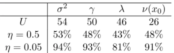
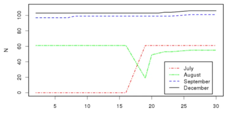
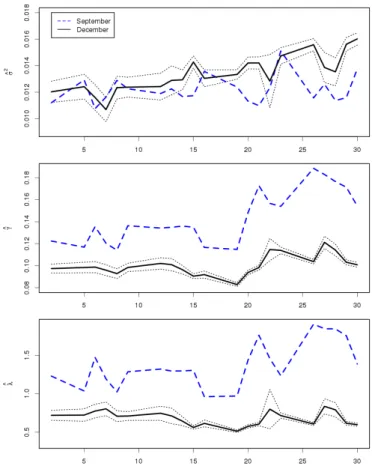
7.5 Finite sample variances of γ,λand ν . . . 82
8 A uniform central limit theorem for deconvolution estimators 87 8.1 The estimator . . . 88
8.2 Statement of the theorem . . . 89
8.3 Discussion . . . 92
8.4 The deconvolution operator . . . 95
8.5 Convergence of the finite dimensional distributions . . . 97
8.5.1 The bias . . . 97
8.5.2 The stochastic error . . . 98
8.6 Tightness . . . 100
8.6.1 Pregaussian limit process . . . 101
8.6.2 Uniform central limit theorem . . . 103
8.6.3 The critical term . . . 105
8.7 Function spaces . . . 108
9 Conclusion and outlook 111
Acknowledgements 115
Bibliography 117
Central limit theorems for estimators are of fundamental interest since they allow to assess the reliability of estimators and to construct confidence sets which cover the unknown parameters or functions with a prescribed probability. We focus on nonpara- metric inverse problems and study two different but related models. In the first one, an asset price is modeled by an exponential of a Lévy process. Option prices of the asset are observed and the aim is to estimate the characteristic triplet of the Lévy process.
The second model is deconvolution, where independent, identically distributed random variables with additive error are observed and the aim is statistical inference on the distribution of the random variables.
In both models, in the estimation of the Lévy process and in the deconvolution, we study central limit theorems for estimators that are based on Fourier methods. In the first set–up, the price of an asset (St) follows under the risk–neutral measure an exponential Lévy model
St=Sert+Lt with a Lévy process (Lt) for t>0,
where S > 0 the present value of the stock and r > 0 is the riskless interest rate.
Based on prices of European options with the underlying (St), we calibrate the model by estimating the characteristic triplet of (Lt), which consists of the volatility, the drift and the Lévy measure. We construct confidence sets for the characteristic triplet. This is of particular importance since the calibrated model is the basis for pricing and hedging.
The calibration problem is closely related to the classical nonparametric inverse problem of deconvolution. On the one hand the law of the continuous part is convolved with the law of the jump part of the Lévy process. On the other hand the Lévy measure is convolved with itself in the marginal distribution of the jump part. Besides being itself an interesting problem with many applications, the deconvolution model exhibits the same underlying structure as the nonlinear estimation of the characteristic triplet of a Lévy process and is easier to analyze since it is linear. In the deconvolution model, we observen random variables
Yj =Xj+εj, j= 1, . . . , n,
where the Xj are identically distributed with density fX, the εj are identically dis- tributed with density fε and where X1, . . . , Xn, ε1, . . . , εn are independent. The aim is to estimate the distribution function of the Xj or, more precisely, linear functionals R ζ(x−t)fX(x) dx of the density fX, where the special case ζ = 1(−∞,0] leads to the estimation of the distribution function. Since the central limit theorems show that the
estimators are asymptotically normally distributed, we also speak of asymptotic normal- ity. In both problems, we determine the joint asymptotic distribution of the estimators.
In the deconvolution problem, we even prove a uniform central limit theorem mean- ing that the asymptotic normality holds uniformly over all t ∈ R. Based on the joint asymptotic distribution of the estimators, we construct confidence intervals and joint confidence sets. The uniform convergence in the deconvolution paves the way for the construction of confidence bands.
Lévy processes are widely used in financial modeling, since they allow to reproduce many stylized facts well. Exponential Lévy models generalize the classical model by Black and Scholes (1973) by accounting in addition to volatility and drift for jumps in the price process. They are capable of modeling not only a volatility smile or skew but also the effect that the smile or skew is more pronounced for shorter maturities. For a recent review on pricing and hedging in exponential Lévy models see Tankov (2011).
The calibration of exponential Lévy models has mainly focused on parametric models, cf. Barndorff-Nielsen (1998); Carr et al. (2002); Eberlein et al. (1998) and the references therein. First nonparametric calibration procedures for Lévy models were proposed by Cont and Tankov (2004b, 2006) as well as by Belomestny and Reiß (2006a). In these approaches no parametrization is assumed on the jump density and thus the model mis- specification is reduced. In both methods, the calibration is based on prices of European call and put options. Cont and Tankov introduce a least squares estimator penalized by relative entropy. Belomestny and Reiß propose the spectral calibration method and show that it achieves the minimax rates of convergence. The spectral calibration method is designed for finite intensity Lévy processes with Gaussian component and it is based on a regularization by a spectral cut–off. We show asymptotic normality as well as con- struct confidence sets and intervals for the spectral calibration method. Similar methods were also applied by Belomestny (2010) to estimate the fractional order of regular Lévy processes of exponential type, by Belomestny and Schoenmakers (2011) to calibrate a Libor model and by Trabs (2012) to estimate self–decomposable Lévy processes.
The estimation of Lévy processes from direct observations has been studied for high–
frequency and for low–frequency observations. For high–frequency observations the time between observations tends to zero as the number of observations grows, while for low–
frequency observations the time between observations is fixed. As a starting point for high–frequency observations, Figueroa-López and Houdré (2006) estimate a Lévy pro- cess nonparametrically from continuous observations. Nonparametric estimation from discrete observations at high frequency is treated by Figueroa-López (2009) or by Comte and Genon-Catalot (2009, 2011). Nonparametric estimation of Lévy processes from low–
frequency observations has been studied for the estimation of functionals by Neumann and Reiß (2009), for finite intensity Lévy processes with Gaussian component by Gu- gushvili (2009) or for pure jump Lévy processes of finite variation via model selection by Comte and Genon-Catalot (2010) and by Kappus (2012).
We prove asymptotic normality for the spectral calibration method, where the Lévy process is observed only indirectly since the method is based on option prices. The indirect observation scheme does not correspond to direct observations at high frequency
the drift, the intensity and pointwise for estimators of the jump density. These theorems on asymptotic normality belong to the main results of this thesis and are also available in Söhl (2012). This calibration problem is a statistical inverse problem, which is completely different in the mildly ill–posed case of volatility zero and in the severely ill–posed case of positive volatility. We treat both cases. A confidence set is called honest if the level is achieved uniformly over a class of the estimated objects. We prove asymptotic normality uniformly over a class of characteristic triplets and use this to construct honest confidence intervals. The asymptotic normality results are based on undersmoothing and on a linearization of the stochastic errors. As it turns out the asymptotic distribution is completely determined by the linearized stochastic errors.
Based on the asymptotic analysis, we construct confidence intervals from the finite sample variance of the linearized stochastic errors. We study the performance of the confidence intervals in simulations and apply the confidence intervals to option data of the German DAX index. While we focus in this thesis on the spectral calibration method by Belomestny and Reiß (2006a), the approach can be easily generalized to similar methods. The construction of the confidence sets, the simulations and the empirical study will appear in Söhl and Trabs (2012b), where this is also carried out for the method by Trabs (2012).
Nonparametric confidence intervals and sets for jump densities have been studied by Figueroa-López (2011). The method is based on direct high–frequency observations so that the statistical problem of estimating the jump density is easier than in our set–up.
On the other hand the results yield beyond pointwise confidence intervals also confidence bands.
For low–frequency observations, Nickl and Reiß (2012) show in a recent paper a central limit theorem for the nonparametric estimation of Lévy processes. They consider the estimation of the generalized distribution function of the Lévy measure in the mildly ill–posed case for particular situations in which a √
n–rate can be obtained and prove a uniform central limit theorem for their estimators.
So while central limit theorems have been treated in the nonparametric estimation of Lévy processes for low–frequency observations in the mildly ill–posed case, there are to the best of the author’s knowledge no results in the severely ill–posed case and our results are the first for this case.
The estimation of the characteristic triplet from low–frequency observations of a Lévy processes is closely related to the deconvolution problem. Considering the deconvolution problem for two different densities fX andfX yields equation (8.2), namely
F[fX −fX](u) = ϕ(u)−ϕ(u)
ϕε(u) , (1.1)
where ϕand ϕare the characteristic functions of the observations belonging tofX and fX, respectively, andϕεis the characteristic function of the errorsεj. The corresponding formula (2.28) for two characteristic triplets of a Lévy process exhibits the same struc- ture. The difference is that there ϕandϕε are both replaced by the same characteristic
functionϕT of the Lévy process. This is called auto–deconvolution, since the distribution of the errors is replaced by the marginal distribution of the Lévy process itself. From the structure of the above formula one can also see that the decay of the characteristic functionsϕε andϕT, respectively, determines the ill–posedness of the problems. A poly- nomial decay corresponds to the mildly ill–posed case and an exponential decay to the severely ill–posed case.
We consider the deconvolution problem in the mildly ill–posed case, which is the deconvolution problem with ordinary smooth errors. Using kernel estimators, we estimate linear functionalsRζ(x−t)fX(x) dx, which are general enough to include the estimation of the distribution function as a special case. Our main result in the deconvolution problem is a central limit theorem for the estimators uniformly over all t ∈ R. This result will appear in Söhl and Trabs (2012a), where in addition also the efficiency of the estimators is shown. Similarly to the situation considered by Nickl and Reiß (2012) for Lévy processes, we treat the case where a √
n–rate can be obtained. Our work gives a clear insight into the interplay between the smoothness ofζ and the ill–posedness of the problem. A √
n–rate can be obtained whenever the smoothness of ζ in an L2–Sobolev sense compensates the ill–posedness of the problem determined by the polynomial rate by which the characteristic function of the error decays. The limit processGin the uniform central limit theorem is a generalized Brownian bridge, whose covariance depends on the functionalζ and through the deconvolution operatorF−1[1/ϕε] also on the distribution of the error. By uniform convergence the kernel estimator of fX fulfills the ‘plug–in’
property of Bickel and Ritov (2003). The theory of smoothed empirical processes as treated in Radulović and Wegkamp (2000) as well as in Giné and Nickl (2008) is used to prove the uniform central limit theorem.
Deconvolution is a well studied problem. So we focus here only on the closely related literature and refer to the references therein for further reading. Fan (1991b) treats minimax convergence rates for estimating the density and the distribution function. Bu- tucea and Comte (2009) treat the data–driven choice of the bandwidth for estimating linear functionals of the density fX, but assume some minimal smoothness and inte- grability conditions on the functional, which exclude, for example, the estimation of the distribution function since1(−∞,t] is not integrable. Dattner et al. (2011) study the minimax–optimal and adaptive estimation of the distribution function.
In view of our work, we focus now on asymptotic normality and on confidence sets.
Deconvolution is generally considered in the mildly ill–posed case of ordinary smooth errors and in the severely ill–posed case of supersmooth errors. In ordinary smooth deconvolution, asymptotic normality is shown for the estimation of the density by Fan (1991a) and on slightly weaker assumptions by Fan and Liu (1997). For the estimation of the distribution function, Hall and Lahiri (2008) show asymptotic normality in ordinary smooth deconvolution. In supersmooth deconvolution, asymptotic normality is proved for estimators of the density by Zhang (1990) and by Fan (1991a). Zhang (1990) covers also estimators of the distribution function and van Es and Uh (2005) further determine the asymptotic behavior of the variance for estimators of the density and of the dis- tribution function in supersmooth deconvolution. The asymptotic normality results on
characteristic function of the errors decays exponentially but possibly slower than the one of the Cauchy distribution. Further developing the work by Bickel and Rosenblatt (1973) on density estimation, Bissantz et al. (2007) construct confidence bands for the density in ordinary smooth deconvolution. Lounici and Nickl (2011) give uniform risk bounds for wavelet density estimators in the deconvolution problem, which can be used to construct nonasymptotic confidence bands.
In both problems, we apply spectral regularization. The higher the frequencies, the more they contribute to the stochastic error. We regularize by discarding all frequencies higher than a certain cut–off value. Since we regularize in the spectral domain, Fourier techniques are used for the estimation methods and their analysis.
Another common feature is that Gaussian processes arise naturally in both problems.
The limit process of the stochastic error in the deconvolution problem is a generalized Brownian bridge. The problem of estimating the characteristic triplet of a Lévy process can be simplified by studying observations in the Gaussian white noise model. Applying the estimation method to this modified observation scheme leads to a Gaussian process.
A bound on the supremum of this Gaussian process is derived which is later used to prove asymptotic normality of the estimators. For the Gaussian processes in both prob- lems, we study boundedness and continuity using Dudley’s theorem and metric entropy arguments. While these are classical topics in the theory of Gaussian processes, we also address the question of hitting probabilities for Gaussian processes or, more generally, for Gaussian random fields. These results on hitting probabilities are of independent interest and are published in Söhl (2010). They are used to show that points are polar for the Gaussian process resulting from the Gaussian white noise model meaning that it does not hit a given point almost surely. This implies that the estimators in the Lévy setting are almost surely well–defined.
In both problems, in the deconvolution and in the estimation of the Lévy process, we use nonparametric estimation methods. The estimation errors can be decomposed into a stochastic and an approximation part. Unlike the bias–variance trade–off sug- gests, we do not try to balance stochastic and approximation error but rather aim for undersmoothing. Then the approximation error is asymptotically negligible and thus the asymptotic distribution is centered around the true value. The asymptotic variance can be easily estimated by means of the already used estimators. In contrast to a bias cor- rection, which often leads to more difficult estimation problems, undersmoothing yields accessible asymptotic distributions and feasible confidence sets.
This thesis is organized as follows. Chapter 2 treats the exponential Lévy model and the spectral estimation method. Chapter 3 studies continuity, boundedness and hit- ting probabilities of a related Gaussian process. Chapter 4 contains the main results on asymptotic normality in the Lévy setting. Chapter 5 treats uniform convergence with respect to the underlying probability measure. In Chapter 6 the asymptotic normality results are applied to confidence sets and to a hypotheses test on the value of the volatil- ity. Chapter 7 contains a finite sample analysis, simulations and an empirical study on the calibration of the exponential Lévy model. Chapter 8 treats the deconvolution model
and is devoted to a uniform central limit theorem for estimators of linear functionals of the density. We conclude and give an outlook on further research topics in Chapter 9.
This chapter introduces the spectral calibration method and begins to analyze the esti- mation error. To this end, we provide some background on Lévy processes in Section 2.1.
We describe the spectral calibration method and a slight modification thereof both by Belomestny and Reiß (2006a,b) in Section 2.2, where we also briefly discuss the struc- tural similarity of the calibration and the deconvolution problem. In Section 2.3, an example of model misspecification is considered. We introduce an error decomposition in Section 2.4 which will be important later for the further analysis of the errors.
2.1 Lévy processes
In this section, we define Lévy processes and summarize some of their properties, which can be found, for example, in the monograph by Sato (1999). Later we will need only one dimensional Lévy processes. Nevertheless, we treat here Lévy processes with values inRd since this causes no additional effort.
Definition 2.1 (Lévy process). AnRd–valued stochastic process (Lt)t>0 on probability space (Ω,F,P) is called aLévy process if the following properties are satisfied:
(i) L0 = 0 almost surely,
(ii) (Lt) has independent increments: for any choice ofn>1 and 06t0 < t1 <· · ·< tn the random variablesLt0, Lt1−Lt0, . . . , Ltn−Ltn−1 are independent,
(iii) (Lt) has stationary increments: the distribution ofLt+s−Ltdoes not depend ont, (iv) (Lt) is stochastically continuous: for allt>0,ε >0, lims→0P(|Lt+s−Lt|> ε) = 0, (v) (Lt) has almost surely càdlàg paths: there exists Ω0 ∈ F withP(Ω0) = 1 such that for allω ∈Ω0,Lt(ω) is right–continuous at allt>0 and has left limits at allt >0.
Example 2.2. (i) A Brownian motion with a deterministic drift (ΣBt+γt) is a Lévy process, where Σ∈Rd×d,γ ∈Rd andBt is ad–dimensional Brownian motion.
(ii) A Poisson process (Nt) of intensity λ > 0 is a Lévy process. More generally, the compound Poisson process (Yt) is a Lévy process, where Yt := PNj=1t Zj with independent, identically distributed random variablesZj, which take values inRd. We note that the sum of two independent Lévy processes is again a Lévy process.
These examples capture the behavior of Lévy processes quite well. Indeed, the Lévy–
Itô decomposition states that any Lévy process can be represented as the sum of three
independent components L = L1+L2+L3, where L1 is a Brownian motion with de- terministic drift, L2 is a compound Poisson process with jumps larger or equal to one andL3 is a martingale representing the possible infinitely many jumps smaller than one, which may be obtained as the limit of compensated compound Poisson processes with jumps smaller than one. We call L1 the continuous part and L2+L3 thejump part of the Lévy process. For a precise formulation of the Lévy–Itô decomposition and a proof we refer to Sato (1999). Another main result on Lévy processes is the Lévy–Khintchine representation, whose statement and proof can be found in the same monograph.
Theorem 2.3(Lévy–Khintchine representation). Let(Lt)be a Lévy process. Then there exists a unique triplet (A, b, ν) consisting of a symmetric positive semi–definite matrix A∈Rd×d, a vectorb∈Rd and a measure ν on Rd satisfying
ν({0}) = 0 and Z
Rd(|x|2∧1)ν( dx)<∞, (2.1) such that for allT >0 and for all u∈Rd
ϕT(u) :=E[eihu,LTi]
= exp
T
−1
2hu, Aui+ihb, ui+ Z
Rd(eihu,xi−1−ihu, xi1{|x|61}(x))ν( dx)
Conversely, let(A, b, ν)be a triplet consisting of a symmetric positive semi–definite ma- trix A ∈Rd×d, a vector b∈Rd and a measure ν on Rd satisfying the properties (2.1), then there exists a Lévy process with characteristic function given by the above equation.
We call A ∈ Rd×d the Gaussian covariance matrix and ν the Lévy measure. The Blumenthal–Getoor index is defined as
α:= inf (
r >0 Z
|x|61
|x|rν( dx)<∞ )
and measures the degree of activity of the small jumps. The jump part of a Lévy process is almost surely of bounded variation on compact sets if and only ifR{|x|61}|x|ν( dx)<∞.
In this case we define the drift γ := b−R{|x|61}xν( dx) ∈ R. (A, γ, ν) is called the characteristic triplet of the Lévy process (Lt). If the intensity λ:=ν(Rd) is finite, then the jump part is a compound Poisson process. For a one dimensional Lévy process we write σ2 instead ofA and call σ>0 the volatility.
2.2 Spectral calibration method
In this section, we introduce the exponential Lévy model and describe the spectral calibration method. A slight modification of the spectral calibration method is also explained. At the end of this section, we discuss the similarity of the calibration and the deconvolution problem.
Exponential Lévy models describe the price of an asset by
St=Sert+Lt with a R–valued Lévy process (Lt) for t>0. (2.2) A thorough discussion of this model is given in the monograph by Cont and Tankov (2004a). Since the method is based on option prices, the calibration is in the risk neu- tral world modeled by a filtered probability space (Ω,F,P,(Ft)). We assume that the discounted price process is a martingale with respect to the risk–neutral measure Pand that underPthe price of the asset (St) follows the exponential Lévy model (2.2), where S >0 is the present value of the asset andr >0 is the riskless interest rate.
A European call option with strike price K and maturity T is the right but not the obligation to buy an asset for priceKat timeT. A European put option is the respective right for selling the asset. We denote by C(K, T) and P(K, T) the prices of European call and put options which are determined by the pricing formulas
C(K, T) =e−rT E[(ST −K)+], (2.3) P(K, T) =e−rT E[(K−ST)+], (2.4) where we used the notion (A)+ := max(A,0). Subtracting (2.4) from (2.3) yields the well known put–call parity
C(K, T)− P(K, T) =S−e−rTK,
where we used that (e−rtSt) is a martingale. By the put–call parity, call prices can be calculated into put prices and vice versa so that the observation may be given by either of them. We fix some T and suppose that the observed option prices correspond to different maturities (Kj) and are given by the value of the pricing formula corrupted by noise:
Yj =C(Kj, T) +ηjξj, j = 1, . . . , n. (2.5) The minimax result in Belomestny and Reiß (2006a) is shown for general errors (ξj) which are independent, centered random variables with Var(ξj) = 1 and supjE[ξj4]<∞.
The observation errors are due to the bid–ask spread and other market frictions. The noise levels (ηj) can be either determined from the bid–ask spread, which indicates by Cont and Tankov (2004a, p. 438/439) how reliable an observation is, or they can be estimated nonparametrically, for example, with the method by Fan and Yao (1998). We transform the observations to a regression problem on the function
O(x) :=
( S−1C(x, T), x>0, S−1P(x, T), x <0,
wherex:= log(K/S)−rT denotes the negative log–forward moneyness. The regression model may then be written as
Oj =O(xj) +δjξj, (2.6)
whereδj =S−1ηj. Since the design may change withn, it would be more precise to index the regression model (2.6) bynj instead of byj only. But for notational convenience we omit the dependence on n.
Denoting byδ0the dirac measure at zero, we define the measureνσ(dx) :=σ2δ0(dx) + x2ν(dx). Its structure in a neighborhood of zero is very natural, since it is most use- ful in characterizing weak convergence of the distribution of the Lévy process in view of Theorem VII.2.9 and Remark VII.2.10 in Jacod and Shiryaev (2003). The measure νσ determines the variance of a Lévy process and is relevant for calculating the ∆ in quadratic hedging as noted in Neumann and Reiß (2009). Volatility and small jumps both contribute to the mass assigned byνσ to a neighborhood of zero. Thus it is difficult to distinguish between small jumps and volatility, in fact Neumann and Reiß (2009) point out in their Remark 3.2 that without further restrictions the volatility cannot be estimated consistently. As in Belomestny and Reiß (2006a) we will resolve this problem by considering only Lévy processes (Lt) with finite intensity and with a Lévy measure, which is absolutely continuous with respect to the Lebesgue measure. Since then the Lévy measure is determined by its Lebesgue density, we will denote the Lebesgue density in the following likewise by ν. Then the Lévy–Khintchine representation in Theorem 2.3 simplifies to
ϕT(u) :=E[eiuLT] = exp T −σ2u2
2 +iγu+ Z ∞
−∞
(eiux−1)ν(x) dx
!!
, (2.7) where we call σ > 0 the volatility, γ ∈ R the drift and ν ∈ L1(R) the jump density with intensity λ := kνkL1(R). We call (σ2, γ, ν) the characteristic triplet of the Lévy process (Lt).
In view of the Lévy–Khintchine representation (2.7) and of the independent incre- ments, the martingale property of (e−rtSt) may be equivalently characterized by
E[eLT] = 1∀T >0 ⇐⇒ σ2 2 +γ+
Z ∞
−∞
(ex−1)ν(x) dx= 0. (2.8)
For a jump density ν we denote by µ(x) := exν(x) the corresponding exponentially weighted jump density. The aim is to estimate the characteristic triplet T = (σ2, γ, µ) (we use both equivalent parametrization of characteristic triplets in µ and ν). We will assume that E[e2LT] is finite, which implies that there is a constant C > 0 such that O(x)6Ce−|x| for all x∈R(Belomestny and Reiß, 2006a, Prop. 2.1). This assumption is equivalent to assuming a finite second moment of the asset price,E[ST2]<∞. ThenO is integrable and we can consider the Fourier transformF O.
In the remainder of this section we present and discuss the spectral calibration method and a slight modification thereof both by Belomestny and Reiß (2006a,b). The method is based on the Lévy–Khintchine representation (2.7) and on an option pricing formula
by Carr and Madan (1999) F O(u) :=
Z ∞
−∞
eiuxO(x) dx= 1−ϕT(u−i)
u(u−i) , (2.9)
which holds on the strip {u∈C|Im(u)∈[0,1]}. We define ψ(u) := 1
T log (1 +iu(1 +iu)F O(u)) = 1
T log(ϕT(u−i))
=−σ2u2
2 +i(σ2+γ)u+ (σ2/2 +γ−λ) +Fµ(u),
(2.10)
where the first equality is given by the pricing formula (2.9) and the second by the Lévy–Khintchine representation (2.7). The second equality holds likewise on the strip {u ∈C|Im(u)∈[0,1]} since there the characteristic functionϕT(u−i) is finite by the exponential moment of LT in the martingale condition (2.8). This equation links the observations of O to the characteristic triplet that we want to estimate. Let On be an empirical version of the true function O. For example, On can be obtained by linear interpolation of the data (2.6). ReplacingObyOnin equation (2.10) yields an empirical version of ψ. For direct observations of the Lévy process at low frequency one could plug in the empirical characteristic function of the observations into equation (2.10) and then proceed as described below. But we will stick to the observations in terms of option prices. So we define the empirical counterpart of ψby
ψn(u) := 1
T log>κ(u)(1 +iu(1 +iu)F On(u)), (2.11)
where the trimmed logarithm log>κ :C\{0} →C is given by log>κ(z) :=
( log(z), |z|>κ log(κ z/|z|), |z|< κ
and κ(u) := exp(−T σmax2 u2/2−4T R)/2∈(0,1). The quantities σmax, R>0 are deter- mined by the class of characteristic triplets in Definition 2.4 below. The logarithms are taken in such a way that ψ and ψn are continuous with ψ(0) = ψn(0) = 0. This way of taking the complex logarithm is called distinguished logarithm, see Theorem 7.6.2 in Chung (1974). We will further discuss the distinguished logarithm especially in connec- tion with the definition ofψnin Chapter 3. Considering (2.10) as a quadratic polynomial inu disturbed by Fµ motivates the following definitions of the estimators for a cut–off valueU >0:
σˆ2:=
Z U
−U
Re(ψn(u))wUσ(u)du, (2.12)
γˆ:=−ˆσ2+ Z U
−U
Im(ψn(u))wUγ(u)du, (2.13)
ˆλ:= σˆ2 2 + ˆγ−
Z U
−U
Re(ψn(u))wλU(u)du, (2.14) where the weight functions wσU,wγU andwλU satisfy
Z U
−U
−u2
2 wUσ(u)du= 1, Z U
−U
uwUγ(u)du= 1, Z U
−U
wλU(u)du= 1, Z U
−U
wUσ(u)du= 0, Z U
−U
u2wUλ(u)du= 0.
(2.15)
The estimator forµis defined by a smoothed inverse Fourier transform of the remainder µ(x) :=ˆ F−1
"
ψn(u) +σˆ2
2 (u−i)2−iˆγ(u−i) + ˆλ
! wµU(u)
#
(x), (2.16)
where wµU is compactly supported. The choice of the weight functions is discussed in Section 7.1, where also possible weight functions are given. The weight functions for all U >0 can be obtained fromwσ1,wγ1,w1λ andwµ1 by rescaling:
wσU(u) =U−3w1σ(u/U), wUγ(u) =U−2wγ1(u/U), wλU(u) =U−1w1λ(u/U), wµU(u) =wµ1(u/U).
Sinceψn(−u) =ψn(u), only the symmetric part ofwσ1,wλ1 and the antisymmetric part of wγ1 matter. The antisymmetric part of wµ1 contributes a purely imaginary part to ˆµ(x).
Without loss of generality we will always assume wσ1,wλ1, w1µ to be symmetric and w1γ to be antisymmetric. We further assume that the supports of wσ1, w1γ, wλ1 and w1µ are contained in [−1,1].
To bound the approximation errors some smoothness assumption is necessary. We assume that the characteristic triplet belongs to a smoothness class given by the following definition, which is Definition 4.1 by Belomestny and Reiß (2006a).
Definition 2.4. For s ∈ N and R, σmax > 0 let Gs(R, σmax) denote the set of all characteristic tripletsT = (σ2, γ, µ) such that (eLt) is a martingale, E[e2LT]6R holds, µiss–times (weakly) differentiable and
σ∈[0, σmax], |γ|, λ∈[0, R], max
06k6skµ(k)kL2(R)6R, kµ(s)kL∞(R)6R.
The assumption T ∈ Gs(R, σmax) includes a smoothness assumption of order son µ leading to a decay of Fµ. To profit from this decay when bounding the approximation error in Section 4.3.3, we assume that the weight functions are of orders, this means
F(w1σ(u)/us),F(wγ1(u)/us),F(w1γ(u)/us),F((1−w1µ(u))/us)∈L1(R). (2.17) A slightly modified estimation method is given in a second paper by Belomestny and Reiß (2006b), which is concerned with simulations and an empirical example. We present
this approach here for completeness and since our simulations and our empirical study are partly based on it. In addition, we will apply the modified method to an example and this will shed some light on misspecification in the next section. As noted, the equation (2.10) holds on the whole strip {u ∈ C|Im(u) ∈ [0,1]}. So instead of using this equation directly one could also shift the equation. A shift by one in the imaginary direction is particularly appealing, since then ν can be estimated directly without the intermediate step of estimating an exponentially scaled version of ν. Applying this shift to (2.10) yields
ψ(u+i) = 1
T log(1−u(u+i)F O(u+i)) = 1
T log(ϕT(u))
=−σ2u2
2 +iγu−λ+Fν(u).
(2.18)
Similar as for equation (2.10), one could also plug in an empirical characteristic function obtained from direct, low–frequency observations here. This is exactly the approach Gugushvili (2009) takes. But we noticeF O(u+i) =F[e−xO(x)](u). Again we substitute O by its empirical counterpartOn and define
ψn(u+i) := 1
T log(1−u(u+i)F[e−xOn(x)](u)). (2.19) So the slightly modified estimators are given by
σe2 :=
Z U
−URe(ψn(u+i))wUσ(u)du, (2.20) eγ :=
Z U
−U
Im(ψn(u+i))wUγ(u)du, (2.21) eλ:=−
Z U
−U
Re(ψn(u+i))wλU(u)du, (2.22) where the weight functions are assumed to satisfy the same conditions (2.15) as before.
The corresponding estimator ofν is
νe(x) :=F−1
"
ψn(u+i) +σe2
2 u2−iγue +λe
! wUν(u)
#
(x), (2.23)
where wνU is compactly supported. Belomestny and Reiß (2006b) proposed the weight functions
wUσ(u) := s+ 3
1−2−2/(s+1)U−(s+3)|u|s(1−2·1{|u|>2−1/(s+1)U}), u∈[−U, U], (2.24) wUγ(u) := s+ 2
2Us+2|u|ssgn(u), u∈[−U, U], (2.25)
wUλ(u) := s+ 1
2(22/(s+3)−1)U−(s+1)|u|s(2·1{|u|<2−1/(s+3)U}−1), u∈[−U, U], (2.26)
wνU(u) := (1−(u/U)2)+, u∈R. (2.27) In order to see the similarity of the estimation of the characteristic triplet of a Lévy process with the deconvolution problem we rewrite (2.18) as
TF((σ2/2)δ000−γδ00−λδ0+ν)(u) = log(ϕT(u)).
In the spectral calibration methodϕT is replaced by an empirical version and then this equation is used to estimate the characteristic triplet. We consider the equation for two different characteristic triplets (σ, γ, ν) and (σ, γ, ν) with intensitiesλandλ, respectively, and obtain
TF(((σ2−σ2)/2)δ000−(γ−γ)δ00 −(λ−λ)δ0+ (ν−ν))(u)
= log(ϕT(u))−log(ϕT(u))
= log
1 +ϕT(u)−ϕT(u) ϕT(u)
≈ ϕT(u)−ϕT(u)
ϕT(u) , (2.28)
where the approximation is valid if the absolute value of the last expression is small.
This formula reveals the deconvolution structure of the problem. On the one hand the similarity with the corresponding formula for deconvolution (1.1) is striking. On the other hand we can see the deconvolution structure directly from formula (2.28). To this end, we multiply withϕT on both sides. Since a multiplication in the spectral domain corresponds to a convolution in the spatial domain, we see that the difference in the characteristic triplet is convolved with the marginal distribution of the Lévy process. To estimate the characteristic triplet a deconvolution problem has to be solved. Interestingly, the marginal distribution of the Lévy process appears twice, it takes the place of both, the error distribution and the distribution of the observations in the deconvolution problem.
This phenomenon is calledauto–deconvolution.
The linearization of the logarithm in (2.28) will be important later, when we substitute the logarithm (2.31) in the stochastic errors by its linearization (2.32). ThenϕT will be an empirical version of the characteristic function ϕT, which justifies the assumption that ϕT and ϕT are close. The division by the possibly decaying function ϕT is taken care of in the estimation method by the spectral cut–off.
2.3 The misspecified model
We have chosen a nonparametric estimation method to reduce the error due to model misspecification and assume in general that the misspecification error is negligible. Nev- ertheless, model misspecification is an important issue to address. In this section, we want to study at least by means of an example how the misspecified model behaves.
The spectral calibration method is designed for finite intensity Lévy processes. Sudden changes in the price process are incorporated into the model by jumps of the Lévy pro- cess. The Gaussian component models the small fluctuations happening all the time.
Alternatively, one can interpret these fluctuations to be caused by infinitely many small
jumps. This can be modeled by an infinite intensity Lévy process and empirical inves- tigations indicate that Lévy processes with Blumenthal–Getoor index larger than one are particularly suitable. Stable processes allow to consider different Blumenthal–Getoor indices α ∈ (0,2). So we consider a symmetric stable process with additional drift and Gaussian component and study the behavior of the estimators for such a process. The characteristic function is given by
ϕT(u) = exp(T(−σ2u2/2−ηα|u|α+iγu)),
whereα∈(0,2),σ, η >0 andγ ∈R. It holdsψ(u+i) =−σ2u2/2−ηα|u|α+iγu. We take the weight functions wσU, wUγ and wUλ as in (2.24), (2.25) and (2.26), respectively, and wUν =1[−U,U]. We apply the second method given by (2.20)–(2.23) directly to ψ(u+i) and not to its empirical counterpart ψn(u+i) and obtain
σe2= Z U
−U
Re(ψ(u+i))wUσ(u)du=σ2+2−2(s+1−α)/(s+1)
1−2−2/(s+1)
s+ 3
s+α+ 1ηαU−(2−α), eγ=
Z U
−U
Im(ψ(u+i))wγU(u)du=γ, λe=−
Z U
−U
Re(ψ(u+i))wλU(u)du= 2(2−α)/(s+3)−1 22/(s+3)−1
s+ 1
s+α+ 1ηαUα, ν(0) =e F−1[(ψ(u+i) +σe2u2/2−ieγu+λ)1e [−U,U](u)](0)
= (−ηαUα+1/(α+ 1) + (σe2−σ2)U3/6 +λUe )/π.
We observe that the driftγ is estimated correctly. The estimated volatilityσe2 converges with rate U−(2−α) toσ2. The estimated jump intensity is finite, but grows as Uα. The estimated jump intensity at zero ν(0) grows ase Uα+1. Although the estimated jump intensities are always finite, the infinite intensity of the Lévy process is reflected in the estimators by growing jump intensities and by peaks of growing height at zero. For a Lévy process of infinite jump intensity, σe2 has to be interpreted as a joint quantity of volatility and small jumps. The corresponding singularity of the jump density is given bycηα/|x|α+1 withc >0. The smoothing by the weight function in the spectral domain corresponds to a kernel smoothing with bandwidth U−1 in the spatial domain. The integral ofx2ν(x) in a neighborhood of zero with sizeU−1 is proportional to
Z U−1
−U−1
x2ν(x)dx= Z U−1
−U−1
cηα|x|1−αdx= 2
2−αcηαUα−2.
We see that σe2 behaves as the mass assigned by νσ to a neighborhood of zero with size proportional to U−1. This example shows that with the above interpretation the estimators can give valuable information about the process even in the case of model misspecification.
2.4 Preliminary error analysis
In this section, we start with a preliminary analysis of the error in the correctly specified model. We decompose the error into an approximation error and a stochastic error. The stochastic error is further decomposed into a linearized part and a remainder term. The linearized stochastic error is considered in the Gaussian white noise model. This leads to the definition of the Gaussian process studied in Chapter 3. At the same time this error decomposition lays the ground for the proof of the asymptotic normality in Chapter 4.
We define the estimation error ∆ˆσ2 := ˆσ2−σ2and likewise for the other estimators. We will also use the notation ∆ψn:=ψn−ψ. The estimation error ∆ˆσ2 can be decomposed as
∆ˆσ2 : = 2 U2
Z 1 0
Re(Fµ(U u))wσ1(u)du+ 2 U2
Z 1 0
Re(∆ψn(U u))w1σ(u)du. (2.29) The first term is the approximation error and decreases in the cut–off valueU due to the decay ofFµ. The second is the stochastic error and increases inU by the growth of ∆ψn. For growing sample size n the term ∆ψn becomes smaller so that the stochastic error decays even if we letU → ∞asn→ ∞. Forσ= 0 the term ∆ψn(u) grows polynomially in u so that we can let U tend polynomially to infinity, whereas for σ > 0 it grows exponentially in u and we can let U tend only logarithmically to infinity. This is the reason for the polynomial and logarithmic convergence rates in the casesσ= 0 andσ >0, respectively. For fixed sample size the cut–off valueU is the crucial tuning parameter in this method and allows a trade–off between the error terms. The influence of the cut–
off valueU is analogous to the influence of the bandwidth h on kernel estimators, more preciselyU−1corresponds toh. The other estimation errors allow similar decompositions as ∆ˆσ2 in (2.29) and they are given by equations (4.1), (4.2) and (4.3) in the proof of Theorem 4.1.
To simplify the asymptotic analysis of the stochastic errors, we do not work with the regression model (2.6) but with the Gaussian white noise model. This is an idealized observation scheme, where the terms are easier to analyze. At the same time asymptotic results may be transferred to the regression model. The Gaussian white noise model is given by
dZn(x) =O(x)dx+nδ(x)dW(x), x∈R, (2.30) where W is a two–sided Brownian motion, δ ∈ L2(R) and n > 0. In the case of equidistant design the precise connection to the regression model (2.6) is given by δ(xj) = δj and n = n+1n−1(xn−x1)n−1/2, where x1 and xn are the minimal and maxi- mal design points and where we assume that the range of observations (xn−x1) grows slower than n1/2 such that n → 0 as n → ∞. Transferring asymptotic results from the Gaussian white noise model to the regression model is formally justified by Le Cam’s concept of asymptotic equivalence, see Le Cam and Yang (2000). In particu- lar, it can be used to transfer lower bounds and confidence statements. Brown and Low (1996) show that the regression (2.6) with Gaussian errors is asymptotically equiva-