SFB 649 Discussion Paper 2011-073
Calibration of self- decomposable Lévy
models
Mathias Trabs*
* Humboldt-Universität zu Berlin, Germany
This research was supported by the Deutsche
Forschungsgemeinschaft through the SFB 649 "Economic Risk".
http://sfb649.wiwi.hu-berlin.de ISSN 1860-5664
SFB 649, Humboldt-Universität zu Berlin Spandauer Straße 1, D-10178 Berlin
S FB
6 4 9
E C O N O M I C
R I S K
B E R L I N
Calibration of self-decomposable L´evy models
Mathias Trabs∗
Institute for Mathematics, Humboldt-Universit¨at zu Berlin, Germany,trabs@math.hu-berlin.de.
We study the nonparametric calibration of exponential, self-decomposable L´evy models whose jump density can be characterized by the k-function, which is typically nonsmooth at zero. On the one hand the estimation of the drift, the activity measureα:=k(0+) +k(0−) and analog parameters for the derivatives are considered and on the other hand we estimate the k-function outside of a neighborhood of zero. Minimax convergence rates are derived, which depend on α. Therefore, we construct estimators adapting to this unknown parameter. Our estimation method is based on spectral representations of the observed option prices and on regularization by cutting off high frequencies. Finally, the procedure is applied to simulations and real data.
Keywords: adaptation, European option, infinite activity jump process, minimax rates, non linear inverse problem, self-decomposability.
AMS Classification (2010):60G51, 62G20, 91B25.
JEL Classification: C14, G13.
1. Introduction
Since Merton [20] introduced his discontinuous asset price model, stock returns were frequently described by exponentials of L´evy processes. A review of recent pricing and hedging results for these models is given by Tankov [25]. The calibration of the underly- ing model, that is in the case of L´evy models the estimation of the characteristic triplet (σ, γ, ν), from historical asset prices is mostly studied in parametric models only. Re- markable exceptions are the nonparametric penalized least squares method of Cont and Tankov [10] and the spectral calibration procedure of Belomestny and Reiß [3]. Both articles concentrate on models of finite jump activity. Our goal is to extend their re- sults to infinite intensity models. More precisely, we study pure-jump self-decomposable L´evy processes. For instance, this class was considered in the hyperbolic model (Eberlein, Keller and Prause [11]) or the variance gamma model (Madan and Seneta [19]). More- over, self-decomposable distributions are discussed in the financial investigation using Sato processes (Carr et al. [8], Eberlein and Madan [12]). Our results can be applied in this context, too. The nonparametric calibration of L´evy models is not only relevant for stock prices, for instance, it can be used for the Libor market as well (see Belomestny and Schoenmakers [4]). In the context of Ornstein-Uhlenbeck processes, the nonparamet-
∗The author thanks Markus Reiß and Jakob S¨ohl for providing many helpful ideas and comments.
The research was supported by the Collaborative Research Center 649 “Economic Risk” of the German Research Foundation (Deutsche Forschungsgemeinschaft).
1
ric inference of self-decomposable L´evy processes was considered by Jongbloed, van der Meulen and van der Vaart [15].
The jump density of self-decomposable processes can be characterized by ν(x) =k(x)
|x| , x∈R\ {0}, (1.1)
with a non-negative so-called k-function k: R\ {0} →R+ which increases on (−∞,0) and decreases on (0,∞). While the Blumenthal-Getoor index, which was estimated by Belomestny [1], is zeroin our model, the infinite activity can be described on a finer scale by the parameter
α:=k(0+) +k(0−).
Sincekis typically nonsmooth at zero, we face two estimation problems: Firstly, to give a proper description of k at zero, we propose estimators forα and its analogs for the derivatives k(j)(0+) +k(j)(0−), with j ≥ 1, as well as for the drift γ, which can be estimated similarly. We prove convergence rates for their mean squared error which turn out to be optimal in minimax sense up to a logarithmic factor that depends on the precise setup. Secondly, we estimate the shape of the k-function outside of a neighborhood of zero. To this end, we construct an explicit estimator ofkwhose mean integrated squared error on the setR\[−τ, τ], for any τ >0, converges with nearly optimal rates.
Owing to bid-ask spreads and other market frictions, we observe only noisy option prices. The definition of the estimators is based on the relation between these prices and the characteristic function of the driving process established by Carr and Madan [6] and on different spectral representations of the characteristic exponent. Smoothing is done by cutting off all frequencies higher than a critical value depending on a maximal permitted parameterα. The whole estimation procedure is computationally efficient and achieves good results in simulations and in real data examples.
All estimators converge with a polynomial rate, where the maximalαdetermines the ill-posedness of the problem. Assuming sub-Gaussian error distributions, we provide an estimator withα-adaptive rates. The main tool for this result is a concentration inequality for our estimator ˆαwhich might be of independent interest.
This work is organized as follows: In Section 2 we describe the setting of our estimation procedure and give some details about self-decomposable processes. Subsequently, we derive the necessary representations of the characteristic exponent in Section 3. The estimation procedure is described in Section 4, where we also determine the convergence rates of our estimators. The construction of theα-adaptive estimator ofαis contained in Section 5. In view of simulations we discuss our theoretical results and the implementation of the procedure in Section 6. Applying the proposed calibration to real data, we compare our method with the spectral calibration of Belomestny and Reiß [3]. All proofs are given in Section 7.
2. The model
2.1. Self-decomposable L´ evy processes
A real valued random variable X has aself-decomposable law if for anyb >0 there is an independent random variableZb such that X =d bX+Zb. Since each self-decomposable distributionµis infinitely divisible (Sato [22, Prop. 15.5]), we can define the correspond- ing self-decomposable L´evy process as the L´evy process whose law at unit time equals µ.
Self-decomposable laws can be understood as the class of limit distributions of converg- ing scaled sums of independent random variables [22, Thm. 15.3]. This characterization is of economical interest. If we understand the price of an asset as an aggregate of small independent influences and release from the√
nscaling, which leads to diffusion models, we automatically end up in a self-decomposable price process. Owing to the infinite ac- tivity, the features of market prices can be reproduced even without a diffusion part (cf.
Carr et al. [7]). Examples of pure-jump and self-decomposable models for option pricing are the variance gamma model, studied by Madan and Seneta [19] and Madan, Carr and Chang [18], and the hyperbolic model introduced by Eberlein, Keller and Prause [11].
Sato [22, Cor. 15.11] shows that the jump measure of a self-decomposable distribution is always absolutely continuous with respect to the Lebesgue measure and its density can be characterized through equation (1.1). Note that self-decomposability does not affect the volatilityσnor the driftγof the L´evy process.
Assumingαto be finite andσ= 0, the process Xt has finite variation and the char- acteristic function ofXT is given by the L´evy-Khintchine representation:
ϕT(u) :=E[eiuXT] = exp T
iγu+ Z ∞
−∞
|eiux−1|k(x)
|x| dx
. (2.1)
Motivated by a martingale argument, we will suppose the exponential moment condition E[eXt] = 1 for all t≥0, which yields
0 =γ+ Z ∞
−∞
(ex−1)k(x)
|x| dx. (2.2)
In particular, we will imposeR∞
−∞(ex−1)k(x)|x| dx <∞. In this case ϕT is defined on the strip{z∈C|Imz∈[−1,0]}.
Besides L´evy processes there is another class that is closely related to self-decompos- ability. Dropping the condition of stationary increments while retaining the other prop- erties of L´evy processes, we obtain so-called additive processes. An additive process (Yt) which is additionally self-similar, that means for alla >0 it satisfies (Yat)= (ad HYt), for some exponentH >0, is calledSato process. Sato [21] showed that self-decomposable dis- tributions can be characterized as the laws at unit time of self-similar additive processes.
From the self-similarity and self-decomposability follows forT >0 ϕYT(u) =E[eiuYT] =E[eiTHuY1] = exp
iTHγu+ Z ∞
−∞
(eiux−1)k(T−Hx)
|x| dx .
Since our estimation procedure only depends through equation (2.1) on the distributional structure of the underlying process, we can apply the estimators directly to Sato processes using
Ts= 1, γs=THγ, and ks(·) =k(T−H•) instead ofT,γ andkin the case of L´evy processes.
Going back to a L´evy process (Xt), the parameterαcaptures many of its properties such as the smoothness of the densities of the marginal distributions [22, Thm. 28.4] and the tail behavior of the characteristic function of a self-decomposable distribution. Since the stochastic error in our model is driven by|ϕT(u−i)|−1, we prove the following lemma in the appendix.
Lemma 2.1. Let (Xt)be a self-decomposable L´evy process with σ= 0and k-function ksuch that the martingale condition (2.2)is valid.
i) If kexk(x)kL1 < ∞ then there exists a constant Cϕ = Cϕ(T,kexk(x)kL1, α) > 0 such that for all u∈Rwith|u| ≥1 we obtain the bound
|ϕT(u−i)| ≥Cϕ|u|−T α.
ii) Letα, R >¯ 0 then the constantCϕ(T, R,α)¯ holds uniformly for all functionskwith α≤α¯ andkexk(x)kL1≤R.
2.2. Asset prices and Vanilla options
Letr≥0 be the riskless interest rate in the market andS0>0 denote the initial value of the asset. In an exponential L´evy model the price process is given by
St=S0ert+Xt,
whereXtis a L´evy process described by the characteristic triplet (σ, γ, ν). Throughout these notes, we assume Xt to be self-decomposable with σ = 0 and α < ∞. On the probability space (Ω,F,P) with pricing (or martingale) measurePthe discounted process (e−rtSt) is a martingale with respect to its natural filtration (Ft). This property is equivalent toE[eXt] = 1 for allt≥0 and thus, the martingale condition (2.2) holds.
At timet = 0 the risk neutral price of an European call option with underlyingS, time to maturityT and strike price Kis given by
C(K, T) =e−rTE[(ST −K)+],
whereA+:= max{0, A}. Similarly, an European put has the priceP(K, T) =e−rTE[(K−
ST)+]. In terms of the negative log-forward moneynessx:= log(K/S0)−rT the prices can be expressed as
C(x, T) =S0E[(eXT −ex)+] and P(x, T) =S0E[(ex−eXT)+].
Carr and Madan [6] introduced the option function O(x) :=
S0−1C(x, T), x≥0, S0−1P(x, T), x <0 and set the Fourier transformF O(u) :=R∞
−∞eiuxO(x) dxin relation to the characteristic functionϕT through the pricing formula
F O(u) =1−ϕT(u−i)
u(u−i) , u∈R\ {0}. (2.3) The properties ofO were studied further by Belomestny and Reiß [3, Prop. 2.1]: At any x∈ R\ {0} the function O is twice differentiable with R
R|O00(x)|dx ≤3 and the first derivativeO0has a jump of height -1 at zero. Additionally, they showed that Assumption 1 ensures an exponential decay of the option function, i.e.|O(x)|.e−|x|holds forx∈R. Assumption 1. We assume that C2 := E[e2XT] is finite, which is equivalent to the moment conditionE[St2]<∞.
Our observations are given by
Oj=O(xj) +δjεj, j= 1, . . . , N, (2.4) where the noise (εj) consists of independent, centered random variables with E[ε2j] = 1 and supjE[ε4j] < ∞. The noise levels δj are assumed to be positive and known. In practice, the uncertainty is due to market frictions such as bid-ask spreads.
3. Representation of the characteristic exponent
Using (2.1) and (2.3), the shifted characteristic exponent is given by ψ(u) := 1
T log(1 +iu(1 +iu)F O(u)) = 1
T log(ϕT(u−i)) (3.1)
=iγu+γ+ Z ∞
−∞
(ei(u−i)x−1)k(x)
|x| dx (3.2)
for u ∈ R. Note that the last line equals zero for u = 0 because of the martingale condition (2.2). Throughout, we choose a distinguished logarithm, that is a version of the complex logarithm such that ψ is continuous with ψ(0) = 0. On the assumption R∞
−∞(1∨ex)k(x) dx <∞1we can apply Fubini’s theorem to obtain ψ(u) =iγu+γ+
Z 1 0
i(u−i)F(sgn(x)k(x))((u−i)t) dt, (3.3)
1We denoteA∧B:= min{A, B}andA∨B:= max{A, B}forA, B∈R.
where the Fourier transformF(sgn·k) is well-defined on{z∈C|Imz∈[−1,0]}.
Typically, the k-function and its derivatives are not continuous at zero. Moreover, for all non-zero k the functionx7→sgn(x)k(x) has a jump at zero. Therefore, the Fourier transform decreases very slowly. Letkbe smooth onR\ {0} and fulfill an integrability condition which will be important later:
Assumption 2. Assumek∈Cs(R\ {0})with all derivatives having a finite right- and left-hand limit at zero and(1∨ex)k(x), . . . ,(1∨ex)k(s)∈L1(R).
Our idea is to compensate those discontinuities by adding a linear combination of the functions
hj(x) :=xje−x1[0,∞)(x), x∈R, j∈N∪ {0}.
Forj≥1 it holdshj ∈Cj−1(R) and allhj are contained inC∞(R\ {0}). Hence, we can findαj, j= 0, . . . , s−2, such that
g(x) := sgn(x)k(x)−
s−2
X
j=0
αjhj(x)∈Cs−2(R)∩Cs(R\ {0}).
These coefficients are given recursively by the following formula, which can be proved by straight forward calculations. We omit the details.
Lemma 3.1. Grant Assumption 2. The factors αj, j = 0, . . . s−2, satisfying g ∈ Cs−2(R)∩Cs(R\ {0}), can be calculated via
αj = 1
j! k(j)(0+) +k(j)(0−)
−
j
X
m=1
(−1)m m! αj−m, especiallyα0=αholds.
Hence, the Fourier transform in (3.3) can be written as F(sgn·k)(z) = Fg(z) + Ps−2
j=0αjFhj(z), where integration by parts yields Fhj(v−ti) =
Z ∞ 0
ei(v+i(1−t))xxjdx= j!
(1−t−iv)j+1, v∈R, t∈[0,1), and|Fg(u)|decreases as |u|−sbecause of the smoothness ofg. From these preparations we derive a representation ofψwhich allows us to estimateγandα0, . . . αs−2. A plug-in approach yields estimators fork(j)(0+) +k(j)(0−), j = 0, . . . , s−2, using Lemma 3.1.
Since we only apply this representation whenψis multiplied with weight functions having roots of degrees−1 at zero, the poles that appear in (3.4) do no harm.
Proposition 3.2. Let s≥2. On Assumption 2 there exist functions D:{−1,1} →C andρ:R\ {0} →Csuch that|us−1ρ(u)|is bounded inuand it holds
ψ(u) =D(sgn(u)) +iγu−α0log(|u|) +
s−2
X
j=1
ij(j−1)!αj
uj +ρ(u), u6= 0, (3.4)
From the proof in Section 7.1 we deduce the form of the mappingD:{−1,1} →C: D(±1) =γ∓iπ
2 −
s−2
X
j=1
(j−1)!αj+
∞
Z
−∞
g(x)ex/2−1 x dx±i
∞
Z
0
F(ex/2g(x))(±v) dv.
Proposition 3.2 covers the cases≥2. Fors= 1 we conclude from (3.2) and the martingale condition (2.2)
ψ(u) =iγu+ Z ∞
−∞
(eiux−1)exk(x)
|x| dx=iγu+i Z u
0
F sgn(x)exk(x)
(v) dv, (3.5) where the last equation follows from Fubini’s theorem on the conditionR∞
−∞exk(x) dx <
∞, which is implied by Assumption 2. Hence,ψis a sum of a constant from the integra- tion, the linear driftiγu and a remainder of order log|u|, which follows from the decay of the Fourier transform as|u|−1(cf. Lemma 7.1). One can even show Corollary B.6 that there exists noL2-consistent estimator of αfors= 1. Therefore, we concentrate on the cases≥2 in the sequel.
Equation (3.5) allows another useful observation. Defining the exponentially scaled k-function
ke(x) := sgn(x)exk(x), x∈R, we obtain by differentiation
ψ0(u) = 1 T
(i−2u)F O(u)−(u+iu2)F xO(x) (u)
1 + (iu−u2)F O(u) =iγ+iFke(u). (3.6) Using this relation, we can define an estimator ofke.
4. Estimation procedure
4.1. Definition of the estimators and weight functions
Given the observations{(x1, O1), . . . ,(xN, ON)}, we fit a function ˜Oto these data using linear B-splines
bj(x) := x−xj−1 xj−xj−1
1[xj−1,xj)+ xj+1−x xj+1−xj
1[xj,xj+1], j= 1, . . . , N, and a functionβ0 withβ00(0+)−β00(0−) =−1 to take care of the jump ofO0:
O(x) =˜ β0(x) +
N
X
j=1
Ojbj(x), x∈R.
We chooseβ0 with support [xj0−1, xj0] where j0 satisfiesxj0−1<0≤xj0. ReplacingO with ˜Oin the representations (3.1) and (3.6) ofψandψ0, respectively, allows us to define their empirical versions through
ψ(u) :=˜ 1 T log
vκ(u)(1 +iu(1 +iu)FO(u))˜ ,
ψ˜0(u) := 1 T
(i−2u)FO(u)˜ −(u+iu2)F xO(x)˜ (u)
vκ(u)(1 +iu(1 +iu)FO(u))˜ , u∈R, whereκis a positive function and we apply a trimming function given by
vκ(z) :C\ {0} →C, z7→
(z, |z| ≥κ, κz/|z|, |z|< κ
to stabilize for large stochastic errors. A reasonable choice of κ will be derived below.
The function ˜ψis well-defined on the interval [−U, U] on the event
A:={ω∈Ω : 1 +iu(1 +iu)F( ˜O(ω,•))(u)6= 0∀u∈[−U, U]} ⊆Ω.
Forω∈Ω\Awe set ˜ψarbitrarily, for instance equal to zero. The more ˜O concentrates around the true functionOthe greater is the probability ofA. S¨ohl [23] shows even that in the continuous-time L´evy model with finite jump activity the identityP(A) = 1 holds.
In the spirit of Belomestny and Reiß [3] we estimate the parameters γ and αj, j = 0, . . . s−2, as coefficients of the different powers ofuin equation (3.4). Using a spectral cut-off valueU >0, we define
ˆ γ:=
Z U
−U
Im( ˜ψ(u))wUγ(u) du and for 0≤j≤s−2
ˆ αj:=
Z U
−U
Re( ˜ψ(u))wUα
j(u) du, ifj is even, Z U
−U
Im( ˜ψ(u))wUα
j(u) du, otherwise.
Owing to (3.6), the nonparametric objectkecan be estimated by ˆke(x) :=F−1
−γˆ−iψ˜0(u) wk(u
U)
(x), x∈R.
The weight functions wγU and wUαj are chosen such that they filter the coefficients of interest. Moreover,wk should decrease fast in the spatial domain and should cut off high frequencies:
Assumption 3. We assume:
• wUγ fulfills for all oddj∈ {1, . . . , s−2}
Z U
−U
uwγU(u) du= 1, Z U
−U
u−jwUγ(u) du= 0 and Z U
0
wUγ(±u) du= 0.
• wUα0 satisfies for all evenj∈ {1, . . . , s−2}
Z U
−U
log(|u|)wαU0(u) du=−1, Z U
−U
u−jwUα0(u) du= 0 and Z U
0
wαU0(±u) du= 0.
• Forj= 1, . . . , s−2 the weight functionswαUj fulfill Z U
−U
u−jwUα
j(u) du=(−1)bj/2c (j−1)! ,
Z U
−U
u−lwUα
j(u) du= 0and Z U
0
wUα
j(±u) du= 0, where 1 ≤ l ≤ s−2 and l is even for even j and odd otherwise. For even j we impose additionally
Z U
−U
log(|u|)wUαj(u) du= 0.
• wk is contained inCm(R)for some m≥2s+ 1and satisfies suppwk ⊆[−1,1]as well as wk ≡1 on(−ak, ak)for someak∈(0,1).
Furthermore, we assume continuity and boundedness of the functions u7→u−s+1wq1(u) forq∈ {γ, α0, . . . , αs−2}.
The integral conditions can be provided by rescaling: Letw1q satisfy Assumption 3 for q∈ {γ, α0, . . . , αs−2} andU = 1. Since 1 =R1
−1uw1γ(u) du=RU
−UuU−2w1γ(u/U) du, we can choosewγU(u) :=U−2w1γ(Uu). Similarly, a rescaling is possible forwUα0:
−1 = Z 1
−1
log(|u|)w1α0(u) du= Z U
−U
log(|u|)U−1wα10(u
U) du−log(U) U
Z U
−U
w1α0(u U) du
= Z U
−U
log(|u|)U−1wα10(u U) du.
Therefore, we define wUα
0(u) := U−1wα1
0(Uu) and analogously wαU
j(u) := Uj−1w1α
j(Uu).
The continuity condition in Assumption 3 is set to take advantage of the decay of the remainderρ. In connection with the rescaling it implies
|wγU(u)|.U−s−1|u|s−1 and |wUαj(u)|.U−s+j|u|s−1, j= 0, . . . , s−2. (4.1) In the sequel we assume that the weight functions satisfy Assumption 3 and the property (4.1).
4.2. Convergence rates
To ensure a well-defined procedure, an exponential decay ofO, the identity (3.5) and to obtain a lower bound of|ϕT(u−i)|, we consider the classG0(R,α). Uniform convergence¯ results for the parameters will be derived in the smoothness classGs(R,α).¯
Definition 4.1. Lets∈NandR,α >¯ 0. We define
i) G0(R,α)¯ as the set of all pairs P = (γ, k) where k is a k-function and the corre- sponding L´evy processX given by the triplet (0, γ, k(x)/|x|)satisfies Assumption 1 with C2≤R, martingale condition (2.2)as well as
α∈[0,α]¯ and kkek ≤R,
ii) Gs(R,α)¯ as the set of all pairsP = (γ, k)∈ G0(R,α)¯ satisfying addionally Assump- tion 2 with
|k(l)(0+) +k(l)(0−)| ≤R, forl= 1, . . . , s−1, k(1∨ex)k(l)(x)kL1 ≤R, forl= 0, . . . , s.
In the classG0(R,α) Lemma 2.1 ii) provides a common lower bound of¯ |ϕT(u−i)|for
|u| ≥1. Using maxx∈R1−cos(x)x ∈(0,1], we estimate roughly foru∈(−1,1)\ {0}:
|ϕT(u−i)|= exp T
Z ∞
−∞
(cos(ux)−1)exk(x) x dx
≥exp
−T Z ∞
−∞
ex/|u|k( x
|u|) dx
≥exp
−T R .
Hence, the choice
κ(u) :=κα¯(u) :=
(1
3e−T R, |u|<1,
1
3Cϕ(T, R,α)|u|¯ −Tα¯, |u| ≥1, satisfies
1
3|ϕT(u−i)| ≥κ(u), u∈R, (4.2) where the factor 1/3 is used for technical reasons. As discussed above, we can restrict our investigation to the cases≥2.
Since the L´evy process is only identifiable if O is known on the whole real line, we consider asymptotics of a growing number of observations with
∆ := max
j=2,...,N(xj−xj−1)→0 and A:= min(xN,−x1)→ ∞.
Taking into account the numerical interpolation error and the stochastic error, we analyze the risk of the estimators in terms of the abstract noise level
ε:= ∆3/2+ ∆1/2kδkl∞.
Theorem 4.2. Let s ≥2, R,α >¯ 0 and assumee−A .∆2 and ∆kδk2l2 . kδk2l∞. We choose the cut-off valueUα¯ :=ε−2/(2s+2Tα+1)¯ to obtain the uniform convergence rates
sup
P=(γ,k)∈Gs(R,¯α)
EP[|ˆγ−γ|2]1/2.ε2s/(2s+2Tα+1)¯ and sup
P=(γ,k)∈Gs(R,¯α)
EP[|αˆj−αj|2]1/2.ε2(s−1−j)/(2s+2Tα+1)¯ , j= 0, . . . , s−2.
As one may expect the rates forαj, j= 0, . . . , s−2,become slower asjgets closer to its maximal value because the profit from the smoothness ofk decreases. Note that the cut-off for all estimators is the same.
Remark 4.3. The proof in Section 7.2 reveals that the condition ∆kδk2l2 .kδk2l∞ is only used to estimate the remainder term. In the cases≥3 our bound is not strict and we can replace the constraint by the weaker one
∆rkδk2l2.kδk4−2rl∞ for somer∈
1,3s+ 2Tα¯−1 2s+ 2Tα¯+ 1 i
.
In this settingδj can be bounded away from 0 ifA increases slowly enough whereas for r= 1 the noiseδj must tend to 0 forxj → ±∞. Otherwise ∆kδk2l2 could not be bounded because of ∆N≥ 2AN N→ ∞.
Forτ ∈(0,12) we study the loss of the exponentially scaled k-function ke in the norm kkekL2,τ :=Z
R\[−τ,τ]
|ke(x)|2dx1/2
.
In contrast toGs(R,α) we assume Sobolev conditions on¯ kein the classHs(R,α) in order¯ to applyL2-Fourier analysis.
Definition 4.4. Let s∈ N andR,α >¯ 0. We define Hs(R,α)¯ as the set of all pairs P = (γ, k) ∈ G0(R,α)¯ satisfying additionally k ∈ Cs(R \ {0}), EP[|XTeXT|] ≤ R for corresponding L´evy processX as well as
|γ| ≤R, and kk(l)e kL2 ≤R, forl= 0, . . . , s.
In the next theorem the conditions onAandδare stronger than for the upper bounds of the parameters which is due to the necessity to estimate also the derivative of ψ.
However, the estimation ofψ0 does not lead to a loss in the rate.
Theorem 4.5. Lets≥1, R,α >¯ 0, τ ∈(0,12)and assume Ae−A.∆2 and∆(kδjk2l2+
∆2k(xjδj)jk2l2) . kδk2l∞. We choose the cut-off value Uα¯ := ε−2/(2s+2Tα+5)¯ . Then we obtain for the risk ofˆke the uniform convergence rate
sup
P=(γ,k)∈Hs(R,¯α)
EP[kkˆe−kek2L2,τ]1/2.ε2s/(2s+2Tα+5)¯ .
Remark 4.6. The convergence rates in the Theorems 4.2 and 4.5 are minimax optimal up to a logrithmic factor, which is shown in Appendix B and C.
5. Adaptation
The convergence rate of our estimation procedure depends on the bound ¯αof the true but unknownα∈R+. Therefore, we construct an α-adaptive estimator. For simplicity we concentrate on the estimation of αitself whereas the results can be easily extended toγ,αj, j= 1, . . . , s−2, andke. In this section we will require the following
Assumption 4. LetR >0,s≥2andα∈[0,α]¯ for some maximalα >¯ 0. Furthermore, we suppose e−A.∆2 and∆kδk2l2 .kδk2l∞.
These conditions only recall the setting in which the convergence rates of our param- eter estimators were proven. Given a consistent preestimator ˆαpre of α, let ˜α0 be the estimator using the data-driven cut-off value and the trimming parameter
U˜ :=Uαˆpre:=ε−2/(2s+2Tαˆpre+1) and (5.1)
˜
κ(u) :=κα¯pre(u) :=
(1
2e−T R, |u|<1,
1
2Cα¯pre|u|−Tα¯pre, |u| ≥1, (5.2) respectively, with ¯αpre:= ˆαpre+|logε|−1. If ˆαpreis sufficiently concentrated around the true value, the adaptation does not lead to losses in the rate as the following proposition shows. Note that the condition ˜α0 ∈ [0,α] is not restrictive since any estimator ˆ¯ α of α∈[0,α] can be improved by using (0¯ ∨α)ˆ ∧α¯ instead.
Proposition 5.1. On Assumption 4 let αˆpre be a consistent estimator which is inde- pendent of the dataOj, j= 1, . . . , N, and fulfills for ε→0 the inequality
P(|ˆαpre−α| ≥ |logε|−1)≤dε2 (5.3) with a constantd∈(0,∞). Furthermore, we supposeα˜0∈[0,α]¯ almost surely. Thenα˜0
satisfies the asymptotic risk bound sup
P∈Gs(R,α)
EP,ˆαpre[|α˜0−α|2]1/2.ε2(s−1)/(2s+2T α+1)
where the expectation is taken with respect to the common distribution PP,ˆαpre of the observationsO1, . . . , ON and the preestimatorαˆpre .
To use ˆα0 on an independent sample as preestimator, we establish a concentration result for the proposed procedure. Therefor, we require (εj) to be uniformly sub-Gaussian (see e.g. van de Geer [27]). That means there are constants C1, C2 ∈ (0,∞) such that the following concentration inequality holds for allt, N >0 anda1, . . . aN ∈R
P
N
X
j=1
ajεj ≥t
≤C1exp
−C2 t2 PN
j=1a2j
. (5.4)
Proposition 5.2. Additionally to Assumption 4 let (εj) be uniformly sub-Gaussian fulfilling (5.4). Then there is a constant c > 0 and for all κ > 0 there is an ε0 ∼ κ(2s+2Tα+1)/(2s−2)¯ , such that for all ε < ε0∧1 the estimatorαˆ0 satisfies
P(|ˆα0−α| ≥κ)≤((7N+ 1)C1+ 2) exp −c(κ2∧κ1/2)ε−(s−1)/(2s+2Tα+1)¯
. (5.5) Concentration (5.5) is stronger than in Proposition 5.1 needed. To apply the proposed estimation procedure, letSpre andS be two independent samples with noise levelsεpre and ε as well as sample sizes Npre and N, respectively. Using Spre for the estimator ˆ
αpre, we construct adaptively ˜α0 onS. We suppose Npre grows at most polynomial in εpre, that is Npre . ε−ppre holds for some p >0. This is fulfilled for polynomially strike distributions with a logarithmically growing domain as considered in Appendix B . To satisfy (5.3), it is sufficient if there exists a powerq >0, which can be arbitrary small, such thatεpre∼εq owing to the exponential inequality (5.5). Usingε2&AN/N≥1/N, we estimate
Npre
N .ε−ppreε2∼ε2−pq→0
forq <2/p. Thus, relatively to all available data the necessary number of observations for the preestimator tends to zero.
6. Discussion and application
6.1. Numerical example
We apply the proposed estimation procedure to the variance gamma model (see [18]). In view of the empirical study of Madan, Carr and Chang [18] we choose the parameters ν ∈ {0.05,0.1,0.2,0.5}, σ = 1.2 and θ = −0.15. The value of γ is then given by the martingale condition (2.2):
γ= 1
νlog(1−θν−σ2ν/2).
According to the different choices ofν, we set ¯α= 40 as maximal value ofα.
The deterministic design of the sample{x1, . . . , xN}is distributed normally with mean zero and variance 1/3. The observationsOjare computed from the characteristic function ϕT using the fast Fourier transform method of Carr and Madan [6]. The additive noise consists of normal centered random variables with variance|δO(xj)|2for some δ >0.
We estimateq ∈ {γ, α0, α1, α2, ke}. Hence, we needs ≥ 4 (see Corollary B.6 ). We used maturityT = 0.25, interest r= 0.06, smoothnesss= 6, sample sizeN = 100 and noise level δ = 0.01, which generates values of ε on average 0.168. The results of our Monte Carlo simulations are summarized in Tables 1 and 2.
In order to apply the estimation procedure, we need to choose the tuning param- eters. Owing to the typically unknown smoothness s, let the weight functions satisfy Assumption 3 for some large valuesmax. The weights for the parameters can be chosen
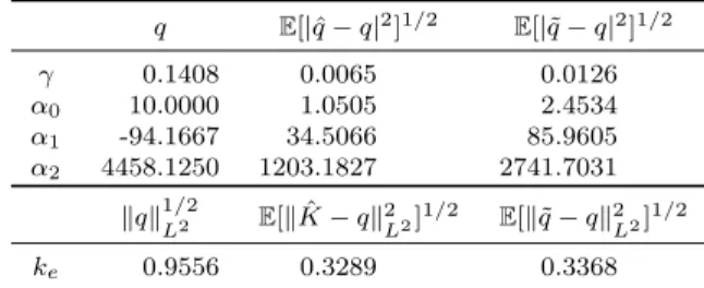
α E[|ˆα0−α|2]1/2 E[|˜α0−α|2]1/2
40 20.7998 23.3589
20 5.8362 7.7724
10 1.0505 2.4534
4 0.1729 1.1158
Table 1. 1000 Monte Carlo simulation of the variance gamma model withN= 100,δ= 0.01 and ν∈ {0.05,0.1,0.2,0.5}.
q E[|ˆq−q|2]1/2 E[|˜q−q|2]1/2
γ 0.1408 0.0065 0.0126
α0 10.0000 1.0505 2.4534
α1 -94.1667 34.5066 85.9605
α2 4458.1250 1203.1827 2741.7031 kqk1/2
L2 E[kKˆ−qk2
L2]1/2 E[k˜q−qk2
L2]1/2
ke 0.9556 0.3289 0.3368
Table 2. 1000 Monte Carlo simulations of the variance gamma model withN= 100,δ= 0.01 and ν= 0.2.
polynomial whereas a flat-top kernel function can be used aswk, as done by Belomestny [2]. The trimming parameterκis included mainly for theoretical reasons and is not im- portant to the implementation. The most crucial point is the choice of the cut-off value U. For ˆq we implement the oracle method U = argminV≥0|ˆq(V)−q| and an adaptive estimator ˜qbased on the construction of Section 5. The sample size for the preestimator is chosenNpre= 25. This adaptation toαis a first step to a data-driven procedure and should be developed further.
6.2. Discussion
The rates show that the studied estimation problem is (mildly) ill-posed compared with classical nonparametric regression models. In order to understand the convergence rate of the estimators forγ andαj better, we rewrite equation (3.6) in the distributional sense, denoting the Dirac distribution at zero byδ0, and differentiate representation (3.4)
ψ0(u) =F iγδ0+ike
(u) =iγ−
s−2
X
j=0
ijj!αju−j−1+ρ0(u), u∈R\ {0}.
Hence,ψ0 can be seen as Fourier transform of an s-times weakly differentiable function and estimatingγfrom noisy observations ofψ0corresponds to a nonparametric regression with regularity s. Since dividing by u on the right-hand side of the above equation corresponds to taking the derivative in the spatial domain, the estimation ofαjis similar to the estimation of the (j + 1)th derivative in a regression model. The convergence rate of ke is in line with the results of Belomestny and Reiß [3] for σ = 0. Outside a
neighborhood of zero estimating the k-function amounts to estimating the jump density itself so that their rates equals ours in the caseα= 0.
For ˆke(x) withxdifferent zero the degree of ill-posedness is given byT α+ 2. This can be seen analytically by observing that the noise is governed by u2|ϕT(u−i)|−1, which grows with rateT α+2. From a statistical point of view a higher value ofαleads to a more active L´evy process and hence, it is harder to distinguish the small jumps of the process from the additive noise. The influence of the time to maturityT on the convergence rates is an interesting deviation from the analysis of Belomestny and Reiß [3]. The simulation shown in Table 1 demonstrates the improvement of the estimation for small the values ofα.
The proposed estimator ˆkedoes not take into account the shape restrictions of the k- function. Therefore, it can be understood as estimator of the function|x|ν(x) for arbitrary absolutely continuous L´evy measures. Thus, the estimation procedure can be applied to exponential L´evy models with Blumenthal-Getoor index larger than zero, for example tempered stable processes. However, the behavior of the L´evy density at zero needs different methods in these cases and should be studied further. For instance, Belomestny [1] discusses the estimation of the fractional order for regular L´evy models of exponential type.
In the self-decomposable framework we reduce the loss of ˆke by truncating positive values on R− and negative ones on R+. The monotonicity can be generated by a re- arrangement of the function. Chernozhukov, Fern´andez-Val and Galichon [9] show that the rearrangement reduces weakly the error for increasing target functions on compact subsets. This result carries over to our estimation problem, whereke is decreasing and we restrict its support to a possibly large interval.
To calibrate the self-decomposable model completely, we combine the estimator ˆke, which works away from zero asymptotically optimal, and the estimators ˆαj, j≥0,which provide a proper description of the true k-function at zero. Using only ˆα0 and ˆα1, this can be done as follows: Choosing someτ >0, we take the estimation of ˆke(x) for|x| ≥τ and extend it continuously with linear functions on (−τ, τ) such that the result fits to ˆ
αj, j= 1,2. We define the combined estimator as
K(x) :=ˆ
m−(x+τ) + ˆke(−τ), −τ < x <0, m+(x−τ) + ˆke(τ), 0≤x < τ, ˆke(x), |x| ≥τ wherem± are uniquely given by the conditions
ˆ
α0= ˆK(0+)−K(0−)ˆ and 2 ˆα0+ ˆα1= ˆK0(0+)−Kˆ0(0−).
Since k is monoton, we force m± ≤ 0, which might lead to a violation of the second equation for large stochastic errors. Table 2 contains simulation results for the estima- tors ˆqand ˜q,q∈ {γ, α0, α1, α2, ke}, corresponding to oracle andα-adaptive cut-off values, respectively. The optimal combination of estimators ˆαj and ˆkeshould be developed fur- ther, for instance an exponential Taylor expansion could be used. However, taking ˆαj
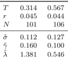
T 0.314 0.567
r 0.045 0.044
Npre 20 21
N 81 85
˜
γ 0.109 0.506
˜
α0 24.850 29.846
˜
α1 -59.595 256.049
˜
α2 9319.844 7570.380
Table 3.. Estimation based on ODAX from 29 May 2008.
Figure 1. Given ODAX data points from 29 May 2008 withT = 0.314 and the option function gen- erated from the estimated model.
for higherj into account leads to a loss in the convergence rate and it is actually not clear how to decompose the estimators into the left and right limits of the derivatives of k. Assuming finite right- and left-hand limits ofk and its derivatives at zero, one-sided kernels might estimate the k-function even in the neighborhood of zero optimally.
Even if the practitioner prefers specific parametric models that might achieve smaller errors and faster rates, the nonparametric method should be used as a goodness-of-fit test against model misspecification. This issue makes progress through study of confidence sets in the framework of L´evy processes with finite activity done by S¨ohl [24] and it would be interesting to derive confidence intervals forα.
6.3. Real data example
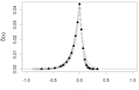
We apply our estimation method to a data set from the Deutsche B¨orse database Eurex2. It consists of settlement prices of put and call options on the DAX index with three and six months to maturity from 29 May 2008. The sample sizes are 101 and 106, respectively.
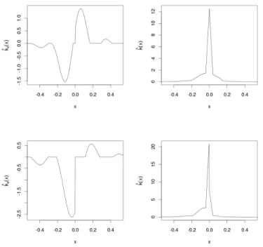
The interest rate is chosen such that the put-call parity holds as best as possible for all pairs of put and call options with the same strike and maturity. The subsample for the preestimator consists of every fifth strike while the main estimation is done from the remaining data points. By a rule of thumb the bid-ask spread is chosen as 1% of the option prices. Therefore, we get noise levelsεwith values 0.0138 and 0.069 for the two maturities, respectively. Table 3 shows the result of the proposed method. The estimations ofkeare presented in Figure 2, which show ˆke without rearrangement as well as the estimated k-function which results from ˆK. In Figure 1 the calibrated model is used to generate the option function in the case of three months to maturity, where the data points used for the preestimator are marked with triangles in the figure.
2provided through the Collaborative Research Center 649 “Economic Risk”
Figure 2. Estimation of ODAX data from 29 May 2008 with three (top) and six (bottom) months maturity.Left: Estimated function ˆke.Right: Estimation of the k-function using ˆK.
Finally, we compare the outcome of our estimation procedure with the spectral calibra- tion of Belomestny and Reiß [3], where the cut-off value is chosen by the penalized least squares criterion. The estimation results of the latter method applied to the same data set are presented in Table 4. We obtain that the higherαin the selfdecomposable model corresponds to a higherσin the L´evy model with finite jump activity. The parameterλ is even smaller forT = 0.567.
7. Proofs
7.1. Proof of Proposition 3.2
Standard Fourier analysis yields the decay of|Fg(u)|:
Lemma 7.1. Letf ∈Cs−2(R)∩Cs(R\ {0})fors≥2 andf ∈C1(R\ {0})in case of s= 1, respectively. Furthermore, we assume finite left- and right-hand limits of f(s−1) andf(s) at zero andf(0), . . . , f(s)∈L1(R). Then we obtain
|Ff(u)|.|u|−s for|u| → ∞.
T 0.314 0.567 r 0.045 0.044
N 101 106
˜
σ 0.112 0.127
˜
γ 0.160 0.100 λ˜ 1.381 0.546
Table 4. Estimation based on ODAX from 29 May 2008.
Especially, on Assumption 2 there is a constantCg >0 independent from t and usuch that
|Fg(v−it)| ≤Cg|v|−s fort∈[0,1)and|v| ≥ 1 2.
Proof. Part 1: Sincef ∈Cs−2(R) has a piecewise continuous (s−1)th derivative and all derivatives are inL1(R), standard Fourier analysis yields
F(f(s−1))(u) = (−iu)s−1Ff(u).
Therefore, it is enough to show forf ∈C1(R\ {0}) with f, f0 ∈L1(R) that|Ff(u)| ≤ C|u|−1,|u| ≥1, where C >0 does not depend onu. The integrability off0 ensures the existence of the limits off forx→ ±∞. Sincef itself is absolutely integrable, those limits equal 0. Integration by parts applied to the piecewiseC1-function verifies foru6= 0:
|Ff(u)|=
Z 0
−∞
eiuxf(x) dx+ Z ∞
0
eiuxf(x) dx = 1
|u||f(0−)−f(0+)− F(f0)(u)|
≤ 1
|u|(|f(0−)−f(0+)|+kf0kL1).
Part 2:From Part 1 and the Leibniz rule follow fort∈[0,1) and|v| ≥ 12
|Fg(v−it)|
= 1
|v|s F
∂s−1
∂xs−1etxg(x)
(v)
g(s−1)(0−)−g(s−1)(0+)− F ∂s
∂xsetxg(x)
(v)
≤ 1
|v|s s−1X
l=0
F
etxg(l)(x) (v)
g(s−1)(0−)−g(s−1)(0+) +
s
X
l=0
F
etxg(l)(x) (v)
.
Hence, it remains to bound |F etxg(l)(x)
(v)| uniformly over t ∈ [0,1) and |v| ≥ 12, wherel= 0, . . . , s. For eachj= 0, . . . s−2 andl = 0, . . . sthere is a linear combination h(l)j (x) =
j
P
m=0
βm(j,l)hm(x) with βm(j,l)∈R, m= 0, . . . , j. Thus, we can findβ(l)j ∈R, j = 0, . . . s−2,such that the derivatives ofg are given by
g(l)(x) = sgn(x)k(l)(x) +
s−2
X
j=0
αjβ(l)j hj(x), x∈R\ {0}, l= 0, . . . , s.
Therefore, we obtain for allt∈[0,1),|v| ≥ 12 andl= 0, . . . , s
F
etxg(l)(x) (v)
=
F
sgn(x)etxk(l)(x) (v) +
s−2
X
j=0
αjβj(l)F etxhj(x) (v)
≤ k(1∨ex)k(l)(x)kL1+
s−2
X
j=0
j!|αjβj(l)|
|1−t−iv|j+1
≤ k(1∨ex)k(l)(x)kL1+
s−2
X
j=0
2(j+1)j!|αjβj(l)|.
With this lemma at hand the representation (3.4) can be proved as follows: Owing to the symmetryψ(−u) =ψ(u), u∈R, it is sufficient to consider the caseu >0. We recall representation (3.3) ofψ:
ψ(u) =iγu+γ+ Z 1
0
i(u−i)F(sgn·k) ((u−i)t) dt.
To develop this integral further we consider forτ∈(0,12) ξτ(u) :=
Z 1−τ 0
i(u−i)F(sgn·k) ((u−i)t) dt
=
s−2
X
j=0
Z 1−τ 0
i(u−i)αjFhj((u−i)t) dt+ Z 1−τ
0
i(u−i)Fg((u−i)t) dt
=−
s−2
X
j=1
(j−1)!αj−α0log(τ−iu(1−τ)) +
s−2
X
j=1
(j−1)!αj
(τ−iu(1−τ))j +
Z 1−τ 0
i(u−i)Fg((u−i)t) dt
To calculate the last integral we split its domain in [0,12] and (12,1−τ]. By assumption and choice ofhj we obtain |ei(u−i)txg(x)| ≤ |(1∨ex/2)g(x)| ∈ L1, for 0≤ t ≤ 12, and thus, we can apply Fubini’s theorem to the first part:
Z 1/2 0
i(u−i)Fg((u−i)t) dt= Z ∞
−∞
g(x) Z 1/2
0
i(u−i)ei(u−i)txdtdx.
Sincez7→eizxis holomorphic, Cauchy’s integral theorem yields Z 1/2
0
i(u−i)ei(u−i)txdt=
Z (u−i)/2 0
ieizxdz= Z −i/2
0
ieizxdz+
Z (u−i)/2
−i/2
ieizxdz.
Hence, Z 1/2
0
i(u−i)Fg((u−i)t) dt= Z ∞
−∞
g(x) Z 1/2
0
etxdt+ Z u/2
0
ieivx+x/2dv
! dx.
Another application of Fubini’s theorem to the second term shows Z 1/2
0
i(u−i)Fg((u−i)t) dt
= Z ∞
−∞
g(x)ex/2−1 x dx+i
Z ∞ 0
F(ex/2g(x))(v) dv−i Z ∞
u/2
F(ex/2g(x))(v) dv. (7.1) The first two summands are independent from u whereas we can use Lemma 7.1 to estimate the last integral foru≥1:
Z ∞ u/2
F(ex/2g(x))(v) dv ≤Cg
Z ∞ u/2
|v|−sdv= 2s−1Cg
s−1 |u|−s+1. (7.2) Also the integral over (12,1−τ] can be estimated using Lemma 7.1. For all τ ∈(0,12) and for allu≥1 we obtain uniformly:
Z 1−τ 1/2
i(u−i)Fg((u−i)t) dt
≤Cg|(u−i)u−s| Z 1
1/2
t−sdt∼ |u|−s+1. (7.3) Thus, (7.1) yields
ξτ(u) =−
s−2
X
j=1
(j−1)!αj+ Z ∞
−∞
g(x)ex/2−1 x dx+i
Z ∞ 0
F(ex/2g(x))(v) dv
−α0log(τ−iu(1−τ)) +
s−2
X
j=1
(j−1)!αj
(τ−iu(1−τ))j +ρτ(u) (7.4) with
ρτ(u) : =−i Z ∞
u/2
F(ex/2g(x))(v) dv+ Z 1−τ
1/2
i(u−i)Fg((u−i)t) dt (7.5)
=−i Z ∞
u/2
F(ex/2g(x))(v) dv+ Z 1−τ
1/2
i(u−i)
F(sgn·k)((u−i)t)
−
s−2
X
j=0
j!αj (1−i(u−i)t)j+1
dt.
Plugging the estimates (7.2) and (7.3) into equation (7.5), we obtain|ρτ(u)|.|u|−s+1 uniformly overτ >0 andu≥1.
For u > 0 there exists ρ(u) := limτ→0ρτ(u) because F(sgn·k) is defined on {z ∈ C|Im(z) ∈[−1,0]} and is continuous on its domain whereas the integral over the sum can be computed explicitly. Then the bound|u|−s+1holds forρ(u),|u| ≥1, too. Also for smallu∈(0,1) the term|us−1ρ(u)|remains bounded sinceρhas a pole at 0 of maximal order s−2. Since all terms in (7.4) are continuous in τ at 0 this equation is true for τ= 0. Finally, we notice log(−iu) = log(| −iu|) +i arg(−iu) = log(|u|)−iπ/2 and insert (7.4) in (3.3).
7.2. Proof of the upper bounds
Let us recall some results of Belomestny and Reiß [3]: Because of the B-spline interpo- lation we obtainOl(x) :=E[ ˜O(x)] =PN
j=1O(xj)bj(x) +β0(x), x∈R. Furthermore, the decomposition of the stochastic error ˜ψ−ψ in a linearizationLand a remainderR,
L(u) :=T−1ϕT(u−i)−1(i−u)uF( ˜O − O)(u), R(u) := ˜ψ(u)−ψ(u)− L(u),
u∈R, has the following properties:
Proposition 7.2. i) Under the hypothesis e−A .∆2 we obtain uniformly over all L´evy triplets satisfying Assumption 1
sup
u∈R
|E[FO(u)˜ − F O(u)]|= sup
u∈R
|F Ol(u)− F O(u)|.∆2.
ii) If the function κ : R → R+ satisfies (4.2) then for all u ∈ R the remainder is bounded by
|R(u)| ≤T−1κ(u)−2(u4+u2)|F( ˜O − O)(u)|2. Upper bound forγ andαj (Theorem 4.2):
Since Theorem 4.2 can be proven analogously to Theorem 4.2 of Belomestny and Reiß [3], we only sketch the main steps. Note that in Gs(R,α) we can bound uniformly the¯ constant Cg from Lemma 7.1. Let us consider γ first. The definition of ˆγ and wγU, the decomposition of ˜ψ and representation (3.4) yield
ˆ γ=
Z U
−U
Im( ˜ψ(u))wUγ(u) du=γ+ Z U
−U
Im(ρ(u) +L(u) +R(u))wUγ(u) du.
Hence, we obtain
E[|ˆγ−γ|2]≤3
Z U
−U
ρ(u)wUγ(u) du
2
+ 3E h
Z U
−U
L(u)wUγ(u) du
2i
+ 3E h
Z U
−U
R(u)wUγ(u) du
2i ,