Deutsche Geodätische Kommission der Bayerischen Akademie der Wissenschaften
Reihe C Dissertationen Heft Nr. 777
Hu Wu
Gravity field recovery from GOCE observations
München 2016
Verlag der Bayerischen Akademie der Wissenschaften in Kommission beim Verlag C. H. Beck
ISSN 0065-5325 ISBN 978-3-7696-5189-8
Diese Arbeit ist gleichzeitig veröffentlicht in:
Wissenschaftliche Arbeiten der Fachrichtung Geodäsie und Geoinformatik der Leibniz Universität Hannover
ISSN 0174-1454, Nr. 324, Hannover 2016
Deutsche Geodätische Kommission der Bayerischen Akademie der Wissenschaften
Reihe C Dissertationen Heft Nr. 777
Gravity field recovery from GOCE observations
Von der Fakultät für Bauingenieurwesen und Geodäsie der Gottfried Wilhelm Leibniz Universität Hannover
zur Erlangung des Grades Doktor-Ingenieur (Dr.-Ing.) genehmigte Dissertation
von
M.Sc. Hu Wu
geboren am 25.09.1986 in Anhui, China
München 2016
Verlag der Bayerischen Akademie der Wissenschaften in Kommission bei der C.H.Beck'schen Verlagsbuchhandlung München
ISSN 0065-5325 ISBN 978-3-7696-5189-8
Diese Arbeit ist gleichzeitig veröffentlicht in:
Wissenschaftliche Arbeiten der Fachrichtung Geodäsie und Geoinformatik der Leibniz Universität Hannover ISSN 0174-1454, Nr. 324, Hannover 2016
Adresse der Deutschen Geodätischen Kommission:
Deutsche Geodätische Kommission
Alfons-Goppel-Straße 11 ! D – 80539 München
Telefon +49 – 89 – 230311113 ! Telefax +49 – 89 – 23031-1283 /-1100 e-mail post@dgk.badw.de ! http://www.dgk.badw.de
Prüfungskommission
Vorsitzender: Prof. Dr.-Ing. Jürgen Müller Korreferenten: Prof. Dr.techn. Wolf-Dieter Schuh
Prof. Dr.-Ing. Christian Heipke Tag der mündlichen Prüfung: 05.07.2016
© 2016 Deutsche Geodätische Kommission, München
Alle Rechte vorbehalten. Ohne Genehmigung der Herausgeber ist es auch nicht gestattet,
die Veröffentlichung oder Teile daraus auf photomechanischem Wege (Photokopie, Mikrokopie) zu vervielfältigen
ISSN 0065-5325 ISBN 978-3-7696-5189-8
Summary
An accurate model of the Earth’s gravity field is beneficial for practical engineering and scien- tific applications, such as the unification of height systems, study of sea-level changes or under- standing of dynamics of the Earth’s interior. In order to improve the knowledge of the gravity field, the dedicated Gravity field and steady-state Ocean Circulation Explorer (GOCE) mission was realized by the European Space Agency (ESA). It was successfully operated from March 2009 to October 2013, and delivered hundreds of millions of observations in this period. In addition to Satellite-to-Satellite Tracking in high-low mode (SST-hl) for the long-wavelength part of the gravity field, the GOCE mission firstly applied Satellite Gravity Gradiometry (SGG) in space to measure the medium- and short-wavelength part. Hence, GOCE provided the great opportunity to recover a gravity field model that is accurate in the full wavelength spectrum down to 100 km spatial resolution.
To recover such a gravity field model, the SST-hl and SGG observations are analysed both separately and jointly. The SST-hl observations are processed with the acceleration approach which balances the satellite accelerations with the first-order derivatives of the gravitational potential, while the SGG observations are directly balanced with the second-order derivatives of the gravitational potential. The separate analysis of the two types of observations leads to two models that are accurate at complementary wavelengths, and the joint analysis gives the final model with high accuracy over the full spectrum up to a spherical harmonic degree 200.
The model determination, i.e., the estimation of the spherical harmonic coefficients, is based on the Least- Squares method. Because of the huge amount of observations and the large number of unknown coefficients, the above-mentioned procedure is a very challenging task with high computational complexity in both time and memory. Also, measurement errors, i.e., outliers, systematic errors and coloured noise, form a big challenge to obtain the best accuracy of the derived model. Moreover, the polar gaps have a severe effect on the zonal and near-zonal coef- ficients. These challenges have been coped with properly to derive a model with high quality.
In addition, the performance of the recovered model is also affected by many other aspects such as the altitude of the satellite, the stochastic model of the observations and the amount of observations. All these issues are fully addressed in this dissertation and solutions are given to provide useful insight for future research.
With a self-developed software written in Fortran, the SST-hl and SGG observations are proces- sed on the cluster system of Leibniz Universit¨at IT Services (LUIS). In addition to two separate models that are accurate in complementary wavelength parts, four generations of combined gravity field models are derived from observations in four time spans (November 2009 - June 2010, November 2009 - April 2011, November 2009 - June 2012, November 2009 - October 2013). The geoid height errors of the four combined models up to a spherical harmonic degree 200 are 3.62, 3.23, 2.98 and 2.75 cm, respectively.
Keywords: GOCE, gravity field model, SST-hl, SGG, outlier, systematic error, coloured noise
iii
Zusammenfassung
Ein genaues Modell des Erdschwerefeldes ist sowohl f¨ur ingenieurpraktische als auch wissen- schaftliche Anwendungen von großem Interesse, wie z.B. bei der Untersuchung von ¨ Anderung- en des Meeresspiegels, der Vereinheitlichung von H¨ohensystemen oder f¨ur das Verst¨andnis der Dynamik des Erdinneren. Um die Kenntnisse ¨uber das Erdschwerefeld weiter zu verbessern, realisierte die European Space Agency (ESA) die GOCE (Gravity field and steady-state Ocean Circulation Explorer) Mission. GOCE umkreiste die Erde zwischen M¨arz 2009 und Oktober 2013 und lieferte in diesem Zeitraum hunderte Millionen von Daten. Neben dem Satellite-to- Satellite Tracking im high-low Modus (SST-hl) zur Bestimmung langwelliger Anteile, wur- de bei der GOCE Mission erstmals die Satellitengradiometrie (Satellite Gravity Gradiometry, SGG) zur Bestimmung mittel- und kurzwelliger Anteile des Erdschwerefeldes genutzt. Damit er¨offnete GOCE die großartige M¨oglichkeit, ein Schwerefeld zu bestimmen, das im gesamten Spektralbereich bis zur r¨aumlichen Aufl¨osung von 100 km hochgenaue Informationen enth¨alt.
Zur Bestimmung eines solchen Schwerefeldmodells werden SST-hl und SGG Beobachtungen sowohl gemeinsam als auch getrennt voneinander analysiert. Die SST-hl Beobachtungen wer- den mit dem Beschleunigungs-Ansatz (acceleration approach) verarbeitet, bei dem die Satel- litenbeschleunigungen mit den ersten Ableitungen des Gravitationspotentials verkn¨upft und ausgeglichen werden. Die SGG Beobachtungen werden ¨uber die direkte Verkn¨upfung zu den zweiten Ableitungen des Gravitationspotentials ausgeglichen. Die getrennte Analyse beider Beobachtungstypen liefert zwei Modelle, die in komplement¨aren Frequenzbereichen genau sind. Die gemeinsame Analyse f¨uhrt zum endg¨ultigen Modell, das eine gute Genauigkeit ¨uber den gesamten Frequenzbereich bis zum sph¨arisch-harmonischen Grad 200 aufweist.
Die Modellbestimmung, also die Sch¨atzung von sph¨arisch-harmonischen Koeffizienten, basiert auf der vermittelnden Ausgleichung nach der Methode der kleinsten Quadrate. Aufgrund der riesigen Anzahl an Beobachtungen und der großen Anzahl an unbekannten Koeffizienten stellt das genannte Verfahren eine sehr anspruchsvolle Aufgabe mit hohem Rechenaufwand in puncto Zeit und Arbeitsspeicher dar. Dar¨uber hinaus ist die Behandlung von Messfehlern, also Aus- reißern, systematischen Fehlern und farbigem Rauschen eine große Herausforderung, um die h¨ochste Genauigkeit des abgeleiteten Modells zu erhalten. Außerdem haben die Polarl¨ocher gravierende Auswirkungen auf die zonalen und nahen zonalen Koeffizienten. Die genannten Herausforderungen wurden zielgerichtet bearbeitet, um ein Modell mit guter Qualit¨at zu be- stimmen. Zus¨atzlich wird die G¨ute des abgeleiteten Modells auch durch viele andere Aspekte, wie beispielsweise die H¨ohe des Satelliten, das stochastische Modell der Beobachtungen und die Anzahl der Beobachtungen, beeinflusst. Alle diese Einflussfaktoren werden ausf¨uhrlich in dieser Arbeit diskutiert, und es werden L¨osungen pr¨asentiert, um wertvolle Hinweise f¨ur zuk¨unftige Forschungsarbeiten zu geben.
Mit einer selbstentwickelten Fortran-Software werden die SST-hl und SGG Beobachtungen auf dem Clustersystem des Leibniz Universit¨at IT Services (LUIS) verarbeitet. Neben zwei separa- ten Modellen, die in komplement¨aren Frequenzbereichen genau sind, werden vier Generationen
v
· vi ·
von kombinierten Schwerefeldmodellen abgeleitet, die sich in Bezug auf die Anzahl der einge- flossenen Beobachtungen unterscheiden (November 2009 - Juni 2010; November 2009 - April 2011; November 2009 - Juni 2012; November 2009 - Oktober 2013). Die Geoidh¨ohenfehler der vier kombinierten und bis zum sph¨arisch-harmonischen Grad 200 aufgel¨osten Modelle ergeben sich zu 3.62, 3.23, 2.98 und 2.75 cm.
Schlagw¨orter: GOCE, Schwerefeldmodell, SST-hl, SGG, Ausreißer, systematische Fehler, far-
biges Rauschen
Contents
1 Introduction 1
1.1 Motivation . . . . 2
1.2 Aim and objectives . . . . 4
1.3 Outline of this work . . . . 5
2 Global gravity field recovery – theory 7 2.1 Gravitational field model and its derivatives . . . . 7
2.2 Least-Squares adjustment . . . . 12
2.2.1 Basis of LS adjustment . . . . 12
2.2.2 Design matrix . . . . 14
2.2.3 Normal matrix . . . . 15
2.2.4 Variance/covariance matrix . . . . 16
2.3 Parameter pre-elimination technique . . . . 17
2.4 Regularization . . . . 19
2.5 Data combination . . . . 20
2.6 Validation of the gravitational field model . . . . 21
2.6.1 Validation in the spectral domain . . . . 21
2.6.2 Validation in the space domain . . . . 23
2.6.3 Validation by GPS leveling . . . . 24
3 Global gravity field recovery from GOCE SST-hl Data 25 3.1 Background of SST-hl technique and related work . . . . 25
3.1.1 SST-hl technique . . . . 25
3.1.2 Related work . . . . 27
vii
· viii · Contents
3.2 Acceleration approach . . . . 30
3.2.1 Theory of the acceleration approach . . . . 30
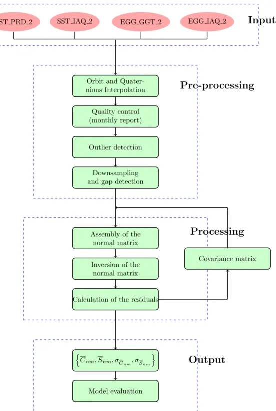
3.2.2 Workflow to process the GOCE SST-hl data . . . . 31
3.3 Data usage . . . . 32
3.4 Data pre-processing . . . . 34
3.4.1 Outlier detection . . . . 34
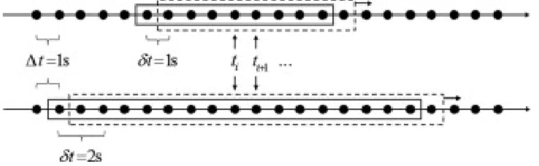
3.4.2 Down-sampling . . . . 36
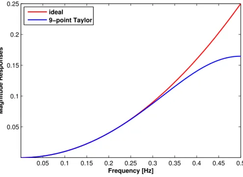
3.4.3 Numerical differentiation . . . . 38
3.4.4 Temporal corrections . . . . 39
3.5 Data processing . . . . 42
3.6 Result Analysis . . . . 46
4 Global gravity field recovery from GOCE SGG data 49 4.1 Technique background and related work . . . . 49
4.1.1 Introduction to gradiometry . . . . 50
4.1.2 Electrostatic Gravity Gradiometer . . . . 51
4.1.3 Overview of the recovering approaches for SGG data . . . . 53
4.2 The workflow of gravity field recovery from SGG data . . . . 55
4.3 Data understanding . . . . 57
4.3.1 Data description . . . . 57
4.3.2 Properties of the gravity gradients . . . . 58
4.3.3 Noise behaviour of the gravity gradients . . . . 62
4.4 Pre-processing of the gravity gradients . . . . 65
4.4.1 Removal of anomalous observations . . . . 65
4.4.2 Detection of outliers . . . . 66
4.4.3 Examination of big data gaps . . . . 67
Contents · ix ·
4.5 Model recovery . . . . 68
4.5.1 Functional model . . . . 68
4.5.2 The main steps of model recovery . . . . 70
4.5.3 Technical challenges . . . . 71
4.6 Result Analysis . . . . 73
4.6.1 Effect of model configurations . . . . 73
4.6.2 Contribution of each component . . . . 76
4.6.3 Results from different amounts of observations . . . . 81
4.6.4 Analysis of the gravity gradients at the lowered orbit . . . . 81
4.6.5 Final models from only gravity gradients . . . . 87
5 Combined gravity field models using all GOCE observations 91 5.1 Combined analysis of different data groups . . . . 91
5.2 Evaluation of the IFE models . . . . 92
5.2.1 Internal evaluation of the IFE models . . . . 93
5.2.2 External evaluation of the IFE models in the frequency domain . . . . . 96
5.2.3 External evaluation of the IFE models in the space domain . . . . 101
6 Conclusions and outlook 105 6.1 Conclusions . . . . 105
6.2 Outlook . . . . 107
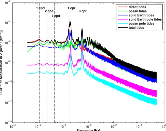
Appendix A Temporal corrections 109 A.1 Direct tides . . . . 109
A.2 Solid Earth tides . . . . 110
A.3 Ocean tides . . . . 112
A.4 Solid Earth pole tides . . . . 113
A.5 Ocean pole tides . . . . 114
· x · Contents
Bibliography 115
List of Figures 123
List of Tables 127
List of Abbreviations 129
Curriculum Vitae 131
Acknowledgements 133
Chapter 1 Introduction
Gravity is a fundamental force of nature that is responsible for many dynamic processes in the Earth’s interior, on and above its surface. The determination of the gravity field thus plays an important role in Earth’s science. On the Earth’s surface, gravity is the resultant of gravitational force and the centrifugal force due to Earth’s rotation. Since the contribution of the centrifugal force is analytical and easy to be computed, the Earth’s gravity field determination is commonly referred to the gravitational field determination.
According to Newton’s law of gravitation, each celestial body generates its own gravitational field. Assuming a spherically symmetrical body, the strength of the gravitational field at a given point is determined by the body’s mass and the distance to the center of the body. Hence, supposing that the Earth is spherically symmetrical, the strength of the gravitational field on the Earth’s surface would be constant. In reality, however, this value varies significantly from place to place due to the irregular shape and the heterogeneous mass distribution of the Earth.
Instead of a perfect sphere, the shape of the Earth is roughly a slightly flattened ellipsoid with lumpy topography. More specifically, the Earth’s radius is 21 km larger at the equator than at the poles, and the height difference between the high mountains and the deep ocean valleys reaches nearly 20 km. In addition, the density of the materials that make up the different layers of the Earth also varies, which further increases the heterogeneity of the gravitational field.
Figure 1.1: Gravity anomalies computed from GOCO03s, showing deviations from the theoretical grav- ity of an idealized smooth Earth, the so-called earth ellipsoid
1
· 2 · Chapter 1. Introduction
An accurate model of the Earth’s gravity field is essential for many Earth sciences. On the one hand, gravity anomalies (deviations between the actual field and an idealised Earth body) actually reflect the mass imbalance and dynamics of the Earth’s interior. Thus, an accurate gravity field model of the Earth can contribute to a better understanding of geophysical and geodynamical processes, thereby benefiting research on plate tectonics, geological phenomena such as volcanoes and earthquakes, and many more. On the other hand, the geoid (i.e. the equipotential surface at mean sea-level of a hypothetical ocean at rest) which serves as vertical reference surface for any topographic features is completely based on the gravity field model.
Hence, an accurate gravity field model will lead to an accurate geoid as well. The accuracy of the geoid is crucial for cases involving small height differences such as in engineering geodesy, or in studies of ice motion, sea-level change, ocean circulation, etc., (Rummel et al., 2002;
Johannessen et al., 2003).
In order to obtain the Earth’s gravity field signal, the European Space Agency (ESA) launched the satellite mission Gravity field and steady-state Ocean Circulation Explorer (GOCE) on March 17, 2009. The GOCE mission enables the mapping of the static Earth’s gravity field in an unprecedented detail. In this context, this dissertation aims to derive an accurate and precise global gravity field model of the Earth from the GOCE observations, thereby contributing to the multiple related research fields. The following sections outline the research motivation, objectives as well as the structure of this dissertation, intending to draw a clear overall picture of this research.
1.1 Motivation
Despite the consensus that an accurate global gravity field model is necessary for many Earth sciences, the current gravity field models that are derived from various observing techniques still have limitations from different perspectives. Before the launch of the dedicated satellite gravity missions starting in 2000, the gravity field models were mainly determined from terres- trial gravimetry, satellite altimetry and satellite tracking observations, and the recovered models were limited in terms of accuracy and resolution due to the limitation of their corresponding observation types. For example, the terrestrial data suffer from insufficient coverage due to operational or political reasons, and have limited accuracy in many parts of the world. Simi- larly, satellite altimetry provides accurate information only for the ocean regions, while satellite tracking observations are only sensitive to the very long-wavelength part of the gravity field.
With such kinds of “flawed” observations, only limited improvements of the recovered model
could be expected with some advanced processing procedures.
1.1. Motivation · 3 ·
Therefore, new observation concepts were required in order to obtain an accurate global gravity field model. The new technology should be able to produce observations that can cover the complete range of the gravity field spectrum down to a short wavelength, and data should be collected all over the Earth. This led to the development of dedicated satellite gravity missions where the gravity sensor (the spacecraft) is installed in a nearly polar orbit at an altitude that is low enough to sense gravity field signals down to short wavelengths and to cover the entire planet within a reasonable time period.
In 2000, the era of dedicated satellite gravity mission began with the launch of the Challenging Minisatellite Payload (CHAMP) satellite (Reigber et al., 2002). CHAMP was operated in a decaying polar orbit with an altitude of about 450 km in the beginning, and the technique of Satellite-to-Satellite tracking in high-low (SST-hl) mode with the Global Navigation Satellite System (GNSS) satellites as “high” counterpart, was firstly realized. The CHAMP mission provided homogeneous observations on a global scale, and led to an improvement of the long- wavelength gravity field with about one order of magnitude (Reigber et al., 2003). However, the nature of gravity attenuation with the altitude prohibited the attainment of high spatial resolution.
To highlight the effect of small-scale features, the idea of differentiation were conceived. Soon, the Satellite-to-Satellite tracking in low-low (SST-ll) mode was firstly applied in the Gravity Recovery And Climate Experiment (GRACE) mission (Tapley et al., 2004) which was launched in 2002. This mission consists of two satellites at the same altitude of about 500 km both in a decaying polar orbit, approximately 220 km apart. The two satellites track each other applying the K-band microwave ranging system and the relative motion between the two satellites is measured with high precision. The GRACE mission has been successfully operated for more than 14 years until now, and delivered millions of observations to the users. Thanks to the huge amount of observations, the best accuracy of the long- and medium-scale features of the Earth’s gravity field have been achieved with GRACE (Mayer-G¨urr et al., 2010). However, due to the relatively high altitude and the configuration (repeat cycle) of the satellites, the spatial resolution of the GRACE mission is still limited.
To counteract the attenuation of the Earth’s gravity field with altitude, the Gravity field and
steady-state Ocean Circulation Explorer (GOCE) mission was successfully realized in 2009
(Floberghagen et al., 2011). In addition to the adoption of the SST-hl technique for the long-
wavelength signal, the GOCE mission also applied gradiometry (differential accelerometry) to
improve the gravity field models in the medium- and high-frequency part. The gradiometer on
board of the GOCE satellite measures the second-order derivatives of the Earth’s gravitational
potential so that the gravity field signals are actually amplified. Moreover, the satellite was
· 4 · Chapter 1. Introduction
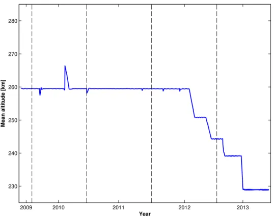
operated at an extremely low altitude of about 250 km which could be realized by a dedicated drag-free control system. The extremely low orbit increased the signal-to-noise ratio of the observations and helped to improve the spatial resolution. Thus, GOCE had the great potential to improve the gravity field in terms of both accuracy and spatial resolution. This dissertation works with the GOCE observations, aiming to derive an accurate (a few centimetres) global gravity field model of the Earth with high spatial resolution down to 80 km (corresponding to a spherical harmonic degree and order of 250) on the Earth’s surface.
1.2 Aim and objectives
The aim of this dissertation is to recover a global gravity field model of the Earth with high accuracy and high spatial resolution from the GOCE observations.
During the entire lifetime of the GOCE mission, the GOCE satellite has returned hundreds of millions of observations. However, recovering a high-accuracy and high-resolution global gravity field model of the Earth from the GOCE observations is still a challenging task. The challenges come from several aspects. First, the huge amount of GOCE observations imposes big efforts in terms of numerical computation. Second, the measurement errors contained in the GOCE observations could damage the quality of the recovered gravity field models and have to be properly dealt with. Third, the polar gaps caused by the inclined orbit of the GOCE satellite have a severe influence on the zonal and near-zonal coefficients. In order to derive an adequate global gravity field model of the Earth, these challenges have to be properly handled.
Numerical computation The Earth’s gravity field model is supposed to be described by tens of thousands of parameters, and these parameters are determined from the hundreds of millions of GOCE observations by Least-Squares (LS) adjustment. In the framework of the LS technique, the assembly and inversion of the normal matrix are the most challenging tasks in terms of computational complexity. For a model truncated at degree and order (d/o) 250, it would take hundreds of days on a single processing unit to assemble the normal matrix for one gravity gradient component, and a memory of about 30 GB to store the normal matrix. Hence, it is hardly feasible to perform the numerical computation on a personal computer. To cope with this challenge, the computation is carried out on the cluster system of Leibniz Universit¨at IT Services (LUIS). In addition, some parallel computation strategy is applied to reduce the computing time, and the Rectangular Full Package format is used to save memory space.
Measurement errors The measurement errors in the GOCE observations include gross errors
(outliers), systematic errors and random errors. They can cause severe problems for the re-
covered gravity field models if they are not properly handled. With the existence of system-
1.3. Outline of this work · 5 ·
atic errors, the detection of outliers is especially challenging. The Observed-Minus-Computed (OMC) observations are used for outlier detection. To absorb systematic errors, the functional models are extended to introduce empirical parameters into each short orbit arc. To reduce the effect of random errors which present a typical coloured noise behaviour, the empirical vari- ance/covariance matrix of the observations is constructed from the initial residuals and then used to de-correlate the observations.
Polar gap The GOCE mission leaves gaps with a radius of 6.5
◦in the polar regions, which severely affects the determination of the zonal and near-zonal coefficients (Sneeuw and van Gelderen, 1997). To handle this issue, some regularization is required. The regularization ma- trix is determined according to Kaula’s rule, while the choice of the regularization parameter that balances the contribution of the observations and the constraints requires extra investiga- tions.
1.3 Outline of this work
The two main types of GOCE observations, i.e., the SST-hl and the SGG observations, are sensitive to different wavelength parts of the Earth’s gravity field signal. To obtain a model that has adequate accuracy over the full wavelength spectrum, the two types of observations are firstly used separately to recover two models that are accurate in different wavelength parts, and then combined together for the recovery of the final model. The processing steps form the main structure of this dissertation.
The dissertation starts, in Chapter 2, with the background of global gravity field modelling as
well as the related theory and algorithms. Firstly, this chapter describes the representation of
the gravitational field and its derivatives, as well as their transformation between different ref-
erence frames. This serves as basis to set up the functional models for the SST-hl and SGG
data processing. Then, the classical LS technique is briefly reviewed. Considering the compu-
tational problem in the GOCE case, special emphasis is put on the theoretical analysis of the
construction of the design matrix, normal matrix and the weight matrix, so that the algorithms
can be optimised for the computation. Further, the functional model is extended by adding
empirical parameters to absorb the systematic errors in the observations, and the corresponding
algorithm, namely the parameter pre-elimination technique, is described thereafter. In addition,
the regularization issue is discussed to cope with the polar gaps and the joint inversion of dif-
ferent data types is addressed. Last but not the least, the strategy to validate the derived models
is described.
· 6 · Chapter 1. Introduction
Chapter 3 discusses the long-wavelength gravity field recovery from the SST-hl observations.
Firstly, the theory of the acceleration approach which is employed in this dissertation is intro- duced. Then, the pre-processing of the SST-hl data is discussed in detail, which includes the outlier detection for the kinematic orbit data, the numerical differentiation algorithm, the so- phisticated down-sampling filters as well as the temporal corrections. With the “clean” input, a GOCE-only long-wavelength gravity field model is derived. The model is then validated in the frequency and space domains.
Chapter 4 discusses the global gravity field recovery from the SGG observations which is sen- sitive to the medium- and short-wavelength part of the gravity field. In the beginning of this chapter, the background and related work of the GOCE SGG data analysis are briefly summa- rized. In the following, the SGG observations are analysed in the time, space and frequency domains in order to achieve a thorough understanding of this new observation type. Then, the pre-processing steps are described, which include the removal of the anomalous observations, the detection of the outliers, and the examination of the data gaps. Thereafter, the processing details are addressed, including the functional model and the computational issues in terms of time and memory. Afterwards, the derived models are analysed to reveal the effects of the model configuration (length of the arc, sampling interval, contribution of the VCMs), each sin- gle gradient component, data volume as well as the orbit altitude. Finally, the models that are purely derived from the gravity gradients are validated.
The combined analysis of SST-hl and SGG data is discussed in Chapter 5. The Variance Com- ponent Estimation (VCE) approach is employed to derive the final gravity field model which covers the full spectrum down to a spatial resolution of 80 km. The derived models reflect four generations depending on different observation time spans. The four generations’ models are validated internally and externally in both the frequency and space domains.
Finally, the results and findings of this research are summarised in Chapter 6, where also direc-
tions for potential future work in global gravity field recovery are identified.
Chapter 2
Global gravity field recovery – theory
This chapter introduces the theoretical background and techniques for global gravity field re- covery. To start with, section 2.1 covers the base functions, i.e., the representations of the grav- itational field and its derivatives, and their transformation between different reference frames.
Together they provide the knowledge required to set up the functional model for gravity field recovery. The GOCE mission has provided a huge amount of observations to generate grav- ity field solutions, while it also poses challenges in several ways. First, the huge amount of observations and large number of unknown parameters form a large-scale linear equation sys- tem, which poses a great numerical challenge to derive the solution. Also, the observations contain unknown systematic errors and polar gaps, which affect the final solution. Moreover, different types of observations have to be analysed in a combined way. To cope with these challenges, section 2.2 explains the Least-Squares (LS) technique to work with this large-scale linear equation system. Considering the complicated case for GOCE, special emphasis is put on the theoretical analysis of the construction of the design matrix, normal matrix and weight matrix so that the algorithms can be optimised for the computation. Section 2.3 discusses an approach to introduce empirical parameters to the functional model to absorb the systematic errors, while section 2.4 addresses the regularization strategy to stabilize the solution of the ill-posed problem caused by the polar gaps. Section 2.5 presents the Variance Component Es- timation (VCE) approach for a combined analysis of different observations types. Finally, the strategy to validate the derived model is addressed in section 2.6.
2.1 Gravitational field model and its derivatives
The gravitational potential V is a harmonic function outside the Earth’s surface that satisfies the Laplace’s equation. As a solution to the Laplace’s equation in the spherical coordinate system, the gravitational potential V can be represented in a harmonic series (Hofmann-Wellenhof and Moritz, 2006) as
V (r, θ, λ) = GM R
∞
X
n=0
( R r )
n+1n
X
m=0
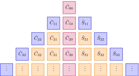
C ¯
nmcos mλ + ¯ S
nmsin mλ P ¯
nm(cos θ), (2.1)
7
· 8 · Chapter 2. Global gravity field recovery – theory
where GM is the gravitational constant of the Earth, R is the equatorial radius of the Earth ref- erence ellipsoid, (r, θ, λ) are the spherical coordinates of a point on the Earth surface (r radius, θ co-latitude, λ longitude), n, m denote spherical harmonic degree and order, P ¯
nm(cos θ) are the fully normalized associated Legendre functions, and C ¯
nm, S ¯
nmare the normalized Spherical Harmonic (SH) coefficients which are the unknowns of the gravity field solution.
This dissertation aims to estimate the SH coefficients from satellite gravimetric observations, e.g., gravity gradients. This process is known as spherical harmonic analysis (Colombo, 1981;
Koop, 1993). In practice, the infinite series expansion is usually truncated at a certain resolv- able degree N
max. On the one hand, the value of N
maxdetermines the spatial resolution D of the recovered gravity field model (D = 20000/N
max, half-wavelength given in km), cf. Jo- hannessen et al. (2003), and a larger N
maxcan reveal more details of the gravitational field.
N
maxis also constrained by the data type. On the other hand, N
maxdetermines the number of coefficients to be estimated by (N
max+ 3)(N
max− 1)
1and thus impacts the computational burden. Hence, the determination of N
maxshould be a balance between benefits and costs.
Reversely, using a set of known potential coefficients, e.g., from a reference gravity field model, the gravitational potential V can be calculated following Eq. (2.1). This is referred as spherical harmonic synthesis (Colombo, 1981; Koop, 1993). With a slight modification to Eq. (2.1), the spherical harmonic synthesis does not only give the gravitational potential but also many other gravity-related quantities such as gravitational accelerations and the gravity gradients, see Eq. (2.2). For example, an a priori signal that has to be subtracted from the original gravimetric observations in the LS adjustment can be modelled from the known highly accurate SH coefficients.
However, the gravitational potential V is not directly measurable. In practice, one often ob- serves gravitational accelerations or gravity gradients
2as alternatives. They correspond to the first- and second-order partial derivatives of the gravitational potential V . In a similar way, gravitational accelerations and gravity gradients can be expressed in a spherical harmonic se- ries by substituting the symbols γ, p, α, β with the corresponding expressions from Table 2.1 (Koop, 1993; Wermuth, 2008),
V
ij= GM R
Nmax
X
n=0
γ ( R r )
n+1n
X
m=0
p [α cos mλ + β sin mλ] . (2.2)
1
The number of the coefficients to be estimated is (N
max+ 1)
2, which excludes the coefficients S ¯
n0as their values are 0. In addition, C ¯
00is usually fixed to 1 and C ¯
10, C ¯
11, S ¯
11are 0 in the case that the origin of the coordinate system coincides with the center of mass of the Earth. Then the total number becomes (N
max+ 3)(N
max− 1).
2
The term “gravity gradients” is widely used in literature instead of “gravitational gradients”, even if the
centrifugal contribution caused by Earth’s rotation is not present, e.g., in space. This terminology is also used in
this dissertation.
2.1. Gravitational field model and its derivatives · 9 ·
Table 2.1: Expressions of the symbols γ, p, α, β in Eq. (2.2) are given. P ¯
nm0, P ¯
nm00denote the first- and second-order derivatives of the Legendre functions w.r.t. θ.
differentiation w.r.t. γ p α β
r −
(n+1)rP ¯
nmC ¯
nmS ¯
nmθ 1 P ¯
nm0C ¯
nmS ¯
nmλ 1 m P ¯
nmS ¯
nm− C ¯
nmrr
(n+1)(n+2)r2P ¯
nmC ¯
nmS ¯
nmrθ −
(n+1)rP ¯
nm0C ¯
nmS ¯
nmrλ −
(n+1)rm P ¯
nmS ¯
nm− C ¯
nmθθ 1 P ¯
nm00C ¯
nmS ¯
nmθλ 1 m P ¯
nm0S ¯
nm− C ¯
nmλλ -1 m
2P ¯
nmC ¯
nmS ¯
nmAlthough modelled in a spherical coordinate system, the gravitational accelerations and the
gravity gradients are actually measured in a Cartesian coordinate system. Also, the practical
work of gravity field recovery involves multiple Cartesian coordinate systems. Hence, the trans-
formations between the spherical coordinate system and Cartesian coordinate systems as well
as among different Cartesian coordinate systems are required. For more details about the trans-
formations between different coordinate systems, the reader is referred to (Koop, 1993). For
the transformations between the spherical coordinate system and Cartesian coordinate systems,
the potential derivatives with respect to the Local North-Oriented reference Frame (LNOF) are
firstly derived. LNOF is a right-handed North-West-Up frame with the X-axis pointing North,
the Y-axis pointing West and the Z-axis Up (EGG-C, 2014). In the following, the transforma-
tion between LNOF and the spherical coordinate system is given in Eq. (2.3) and Eq. (2.4) for
gravitational accelerations and gravity gradients, respectively.
· 10 · Chapter 2. Global gravity field recovery – theory
For the gravitational acceleration components in three directions x, y, z of LNOF (for conve- nience, V
iis written for
∂V∂i), one has
V
x= − 1 r V
θ, V
y= − 1
r sin θ V
λ, V
z=V
r.
(2.3)
And for the gravity gradients V
ijin the LNOF (similarly, V
ijis written for
∂i∂j∂2V), it reads:
V
xx= 1
r V
r+ 1 r
2V
θθ, V
xy= cos θ
r
2sin
2θ V
λ− 1
r
2sin θ V
λθ, V
xz= 1
r
2V
θ− 1 r V
rθ, V
yy= 1
r V
r+ 1
r
2tan θ V
θ+ 1
r
2sin
2θ V
λλ, V
yz= 1
r sin θ V
rλ− 1 r
2sin θ V
λ, V
zz=V
rr.
(2.4)
Eq. (2.3) and (2.4) make it possible to transform gravitational accelerations and gravity gra- dients from the spherical coordinate system to a Cartesian coordinate system, i.e., LNOF. In practice however, instead of LNOF, GOCE observations are delivered in other Cartesian coordi- nate systems, such as the Earth-fixed Reference Frame (ERF, for the orbit) and the Gradiometer Reference Frame (GRF, for gravity gradients). ERF is an orthogonal, right-handed frame with the Z-axis pointing towards the North pole and the X-axis fixed in the equatorial plain in di- rection to the Greenwich meridian, while GRF is an instrumental three-axis coordinate system in which the gravity gradients are observed (EGG-C, 2014). Thus, the transformation among different Cartesian coordinate systems are required.
The gravitational acceleration components constitute a vector, a = [V
xV
yV
z]
T. It can be transformed between different Cartesian coordinate systems according to
a
F2= R
FF21a
F1, (2.5)
where a
F1, a
F2represent the gravitational accelerations in the frames F 1 and F 2; and R
FF21is
the rotation matrix with dimension of 3 × 3 from F 1 to F 2.
2.2. Least-Squares adjustment · 11 ·
The rotation matrix can be obtained in two ways. First, it can be presented as a product of three basic rotation (also called elemental rotation) matrices as
R = R
z(γ)R
y(β)R
x(α), (2.6)
R
z(γ), R
y(β), R
x(α) represent an extrinsic rotation of which the Euler angles α, β, γ are about the axes x, y, z, respectively. For instance, the rotation matrix from LNOF to ERF can be constructed as follows (EGG-C, 2014)
R
ERFLN OF=
− cos θ cos λ sin λ sin θ cos λ
− cos θ sin λ − cos λ sin θ sin λ
sin θ 0 cos θ
, (2.7)
where θ co-latitude and λ longitude of the spacecraft center of mass in ERF.
Alternatively, the rotation information can be obtained with a unit quaternion which provides a convenient mathematical notation for representing an orientation or rotation of objects in three dimensions. In such manner, the rotation matrix is computed as (EGG-C, 2014)
R =
q
20+ q
21− q
22− q
232(q
1q
2− q
3q
0) 2(q
1q
3+ q
2q
0) 2(q
1q
2+ q
3q
0) q
02− q
21+ q
22− q
322(q
2q
3− q
1q
0) 2(q
1q
3− q
2q
0) 2(q
2q
3+ q
1q
0) q
20− q
12− q
22+ q
23
, (2.8)
where (q
0, q
1, q
2, q
3) are the elements of a unit quaternion.
The transformation of gravity gradients is similar, except that the rotation has to be applied twice since the gravity gradients constitute a tensor Γ. More details on the gravity gradient tensor are given in Section 4.1. Thus, the transformation of the gradient tensor is written as
Γ
F2= R
FF21Γ
F1(R
FF21)
T, (2.9) where the gravity gradient tensors in frame F 1 and F 2 are labelled as Γ
F1and Γ
F2, R
FF21represents the rotation matrix, it is the same as that in Eq. (2.5).
The explained knowledge of the base functions as well as the transformations between different
coordinate systems are the building blocks of global gravity field recovery. With them, the
functional models that balance the measurements and the unknown SH coefficients can be set
up for further analysis.
· 12 · Chapter 2. Global gravity field recovery – theory
2.2 Least-Squares adjustment
Modern satellite technology has provided a huge amount of observations to recover a detailed and accurate Earth’s gravity field model that is represented by tens of thousands of parameters.
The huge amount of observations and large number of parameters form a large-scale and over- determined linear equation system. The Least-Squares (LS) technique is employed to solve this large-scale linear system, which poses a great numerical challenge. This section will first briefly introduce the LS adjustment, and then put special emphasis on the construction of the design matrix, normal matrix and weight matrix in order to achieve optimised algorithms for the computations in the GOCE case.
2.2.1 Basis of LS adjustment
For a linear equation system, the functional model that expresses the measurements as a func- tion of the unknown parameters can be represented as
l + v = Ax, (2.10)
where l is the vector of observations, v represents observation residuals, A is the design matrix and x is the vector of unknown parameters. And the stochastic model that describes the accu- racy and correlation of the measurements is represented by a full Variance/Covariance Matrix (VCM) Σ
ll. It reads
Σ
ll=
σ
12σ
12· · · σ
1nσ
21σ
22· · · σ
2n.. . .. . . .. .. . σ
n1σ
n2· · · σ
n2
, (2.11)
where σ
2iis the variance of the i
thmeasurement; σ
ijis the covariance between the i
thand j
thmeasurement.
According to the rule of LS adjustment that minimize the sum of squares of the weighted residuals, the solution x ˆ is estimated by (Koch, 1999)
x ˆ = (A
TP A)
−1A
TP l = N
−1W , (2.12)
where P = Σ
−1llis the weight matrix, N = A
TP A is called the normal matrix, and W =
A
TP l the right hand side of the normal equation N x = W . The normal matrix N is inde-
pendent of the observations since the observations only enter the computation of matrix W .
In fact, N is only determined by the inner geometry of the data distribution. Hence, its in-
2.2. Least-Squares adjustment · 13 ·
verse N
−1is useful in detecting an ill-posed data distribution for the estimation of unknown parameters.
In addition to the estimated parameters x, the residuals ˆ v ˆ after the adjustment ˆ
v = Aˆ x − l (2.13)
have to be computed. Analysing the residuals is a useful tool to assess the quality of the obser- vations. First, the residuals are taken as approximations of the errors so that they can be used to detect outliers in the observations. Then, a Power Spectral Density (PSD) of the residuals can reveal the spectral behaviour of the measurement error. Furthermore, the empirical VCM is computed from the residuals when a priori information of the stochastic model is not avail- able. The residuals are also used to calculate the posterior variance of unit weight σ ˆ
20which is a measure of the quality of the solution. In theory, it is computed from the residuals by
ˆ
σ
20= v ˆ
TP v ˆ
s − r , (2.14)
where s, r are the number of observations and parameters. In practice, however, the large amount of observations would form a rather large design matrix A. The matrix can become so large that it cannot be stored in memory after the adjustment. To avoid a recomputation, instead of Eq. (2.14), σ ˆ
20is actually estimated by
ˆ
σ
02= l
TP l − W
Tx ˆ
s − r . (2.15)
The variance/covariance matrix of the coefficients Σ
xˆxˆis computed by
Σ
xˆxˆ= ˆ σ
02N
−1. (2.16)
The square roots of the diagonal of Σ
xˆxˆgive the standard deviation (formal errors) of the estimated parameters x. Such information is of crucial significance for further use of the model ˆ coefficients in terms of error propagation.
The above gives the theory and basic equations of LS adjustment. However, when applying
them to the GOCE data, one might come across many issues that are caused by the huge amount
of observations and the large number of parameters. These issues will be discussed in the
following subsections.
· 14 · Chapter 2. Global gravity field recovery – theory
2.2.2 Design matrix
The dimension of the design matrix A is s × r, where s and r represent the number of the observations and the estimated parameters, respectively. In the context of GOCE data, s reaches hundreds of millions for one gradient component while r equals (N
max− 1)(N
max+ 3) as explained in the beginning of Section 2.1. Specifically, a gravity field model truncated at d/o 250 has r = 62, 997 unknown parameters. Therefore, the design matrix A stored in a double- precision floating format would require a memory space of more than 50 Terabyte (TB). This is a large storage challenge even to super computers.
One strategy to handle this challenge is storing the much smaller normal matrix N instead of A. This is often used for the recovery of the unknown parameters x, since the recovery of ˆ
ˆ
x is based on the normal equation system. Another strategy is to store the complete matrix A as a list of partitioned blocks A
i, each of which corresponds to one segment of the entire observations. This is also convenient for parallel computation.
With these matrix blocks A
i, the assembly of the normal matrix N becomes (Anton, 2010)
N =A
TP A = h
A
T1A
T2· · · A
Tni
P
10 · · · 0 0 P
2· · · 0 .. . .. . . .. .. . 0 0 · · · P
n
A
1A
2.. . A
n
=A
T1P
1A
1+ A
T2P
2A
2+ · · · + A
TnP
nA
n=N
1+ N
2+ · · · + N
n(2.17)
and similarly,
W = A
T1P
1l
1+ A
T2P
2l
2+ · · · + A
TnP
nl
n= W
1+ W
2+ · · · + W
n. (2.18) Note that in Eq. (2.17), the correlations among each two observation segments are treated as 0.
This is a simplification of the reality, and it can significantly simplify the calculation process.
Hence, the matrices N
iand W
ifor each short segment of the observations can be separately
assembled with efficient parallel computation. And then the complete matrices N and W can
be obtained by summing up their respective partitioned blocks.
2.2. Least-Squares adjustment · 15 ·
2.2.3 Normal matrix
The normal matrix N plays an important role in LS adjustment. First, the unknown parameters can directly be solved based on the normal equation, thus the normal matrix must be assembled and stored. In addition, the inverse of the normal matrix is necessary to estimate the internal quality of the resolved parameters according to Eq. (2.16). Because of the huge number of observations and large number of unknowns, the assembly and inversion of the normal matrix are very numerically challenging. This section gives a theoretical analysis on the computational complexity of N in terms of time and memory.
Assembling the normal matrix N = A
TP A is the most time-consuming task. In the most simplified situation, when P is a unit matrix, N = A
TA. The time complexity for this matrix multiplication is O(sr
2). As discussed in Section 2.2.2, s reaches hundreds of millions for the whole mission period, and r is 62,997 for a model truncated at d/o of 250. In a rough estimate, the assembly of the normal matrix for one gradient component would take more than 500 days on a single-core microprocessor with 10 Giga FLOPS (FLoating-point Operations Per Second, a measure of computer performance). Consequently, it is only feasible to first assemble the partitioned blocks N
ion multiple processors and then retrieve the complete matrix from N
ifollowing Eq. (2.17). As each assembly of N
ican be finished in a few hours (varying with the length of the data segment), this parallelism can significantly improve the computational efficiency. The parallel computation will be carried out on a cluster system, more details are given in Section 4.5.3.
Regarding the solving strategy of unknown parameters, there exist indirect and direct methods.
The indirect method iteratively constructs a series of solution approximations until convergence is achieved. As representatives, the Preconditioned Conjugate Gradient Multiple Adjustment (PCGMA) is discussed in Schuh (1996) and the Least-Square method using QR decomposition (LSQR) is addressed in Baur (2009). By the indirect method, the assembly of the normal matrix can be avoided. In contrast, the direct approach determines the parameters by inversion of the normal matrix. This is also referred to as “brute-force” approach (Roth et al., 2012). A useful feature of the “brute-force” approach is that it can additionally provide the variance/covariance information of the estimated parameters. Therefore in this dissertation, the “brute-force” ap- proach is applied.
With the “brute-force” approach, the estimation is done following three steps. First, decompose
the normal matrix into the product of two triangular matrices, i.e., N = R
TR, where R is an
upper triangular matrix. Among the various decomposition algorithms such as LU, QR, etc., the
most efficient one to solve a symmetric and positive definite matrix (properties of N ) has been
· 16 · Chapter 2. Global gravity field recovery – theory
known as the Cholesky decomposition. The time complexity of the decomposition is O(
13r
3), cf. Intel (2009), where r is the number of the parameters. Next, the parameters x is solved by a straightforward process of backward or forward substitution, the complexity of which is O(r
2) (Intel, 2009). Finally, the inversion of the normal matrix is calculated by N
−1= R
−1(R
−1)
T, and the corresponding complexity is O(
23r
3) (Intel, 2009). Hence, the total time complexity of solving the normal equation by Cholesky decomposition is O(r
3). By a rough estimate, this calculation can be finished in a few of hours on a single-core processor.
Regarding the space complexity, a memory of more than 30 GigaByte (GB) is required to store the complete normal matrix. This is because the matrix has a dimension of r × r, and r is 62,997 for a model truncated at d/o=250. However, the symmetric property of the normal matrix provides an opportunity to save space by storing only the upper or lower triangular part of the matrix. For this purpose, a Rectangular Full Package (RFP) scheme will be introduced in this dissertation, see Section 4.5.3.
2.2.4 Variance/covariance matrix
For independent observations with the same accuracy, their VCM Σ
llwill be a unit matrix and thus negligible in the LS adjustment. However, such premise is not valid for GOCE observa- tions. Because of the widely accepted fact that the errors of the gravity gradients are highly correlated, the VCM of GOCE observations is a full matrix which must be taken into con- sideration. Consequently, the computation complexity is significantly increased for two main reasons. First, the direct storage is impractical because the dimension of VCM is s × s, with the number of observations s being hundreds of millions. Second, it implies an additional op- eration of matrix multiplication to assemble the normal matrix. In this regard, a decorrelation algorithm (Schuh, 2003) is introduced to avoid the direct multiplication of A and Σ
ll.
As the VCM is symmetric and positive definite, it can be decomposed by the Cholesky approach into
Σ
ll= F F
T, (2.19)
where F is a lower triangular matrix. Substituting Eq. (2.19) into the assembly of the normal matrix, one gets
N = A
TP A = A
Tσ
20Σ
−1A = σ
02A
T(F F
T)
−1A = σ
02(F
−1A)
T(F
−1A). (2.20) Define
A ¯ = F
−1A, (2.21)
2.3. Parameter pre-elimination technique · 17 ·
then Eq. (2.20) can be written as
N = σ
02A ¯
TA. ¯ (2.22)
Similarly, the vector W can be rewritten as
W = A
TP l = σ
20A
T(F
−1)
TF
−1l = σ
02(F
−1A)
T(F
−1l) = σ
02A ¯
Tl, ¯ (2.23) where l ¯ = F
−1l. Thus, before assembling of the normal matrix, the design matrix A and the observation vector l are multiplied by the matrix F
−1which can be interpreted as a de- correlated filter process (Schuh, 2003; Pail, 2014). Finally, the solution of the parameters x ˆ is derived by
ˆ
x = N
−1W = (σ
20A ¯
TA) ¯
−1(σ
02A ¯
Tl) = ( ¯ ¯ A
TA) ¯
−1A ¯
Tl. ¯ (2.24) In this dissertation the de-correlated filter F is computed by the Cholesky decomposition of the VCM Σ
ll, and an empirical Σ
llcan be estimated from the observation residuals (see Section 4.3.3) if the true Σ
llis not available. One can also find other methods to design the de-correlated filter F , such as the inverse Fourier transform of the PSD of the residuals, or digital recursive filters like the Auto-Regressive Moving Average (ARMA) filter in the time domain (Kusche and Klees, 2002; Schuh, 2003; Siemes, 2008; Pail, 2014). Nevertheless, all these methods are supposed to obtain similar de-correlated filters.
2.3 Parameter pre-elimination technique
The previous section described the classical LS adjustment that works well under the condition that only stochastic errors exist in the observations. But it does not hold true for the GOCE case. Thus, systematic errors existing in the GOCE orbit and gravity gradient data call for special treatment when applying the LS adjustment. In this regard, the functional model is extended by adding additional parameters to absorb such systematic errors. In contrast to the estimated spherical harmonic coefficients which are commonly named as the aimed parameters or global parameters, these additional parameters are often referred to as empirical parameters or local parameters. Adding empirical parameters into the functional model Eq. (2.10), one will obtain
l + v = A
1x
1+ A
2x
2, (2.25)
where x
1represents the aimed parameters and A
1the corresponding design matrix, x
2, A
2are
empirical parameters and their design matrix. By LS adjustment, the assembly of the normal
· 18 · Chapter 2. Global gravity field recovery – theory
matrix N is written as N =
h
A
1A
2i
TP h
A
1A
2i
=
"
A
T1P A
1A
T1P A
2A
T2P A
1A
T2P A
2#
=
"
N
11N
12N
21N
22# ,
(2.26)
and the right-hand side of the system of normal equations W is written as
W = h
A
1A
2i
TP l =
"
A
T1P l A
T2P l
#
=
"
W
11W
12#
. (2.27)
With the included empirical parameters, the dimension of the normal matrix N becomes (r + p) × (r + p), where r, p are the number of aimed coefficients and empirical parameters, respectively. In a long time span, the number of the empirical parameters may be more than the aimed coefficients. The more empirical parameters are included, the larger the dimension will be, and the more time and space it requires to solve the normal equations, as pointed out in Section 2.2.3.
Since these added empirical parameters are not of real interest for the final solution, here a specific algorithm named Parameter Pre-elimination Technique (Wermuth, 2008; Yi, 2012b) is applied to avoid having to work with the complete normal matrix N . As the name suggests, this technique eliminates the empirical parameters from the normal equations before inversion.
Rewritting the normal equations as
"
N
11N
12N
21N
22# "
x
1x
2#
=
"
W
11W
12#
, (2.28)
one can solve the second equation of Eq. (2.28) for the empirical parameters x
2by
x
2= N
22−1W
2− N
22−1N
21x
1. (2.29) Substituting Eq. (2.29) into the first equation of Eq. (2.28), x
1is then solved by
x
1= (N
11− N
12N
22−1N
21)
−1(W
1− N
12N
22−1W
2). (2.30) Defining
N
∗=N
11− N
12N
22−1N
21, W
∗=W
1− N
12N
22−1W
2,
(2.31)
2.4. Regularization · 19 ·
the dimension of N
∗is the same as N
11which is the normal matrix corresponding to the parameters x
1. When x
1is estimated from Eq. (2.30), the additional parameters x
2can be computed by a back substitution of x
1into Eq. (2.29).
2.4 Regularization
The GOCE satellite runs in a sun-synchronous orbit with an inclination of 96.5
◦, consequently it cannot cover the two polar regions. The absence of observations from the polar regions is called polar gaps (Sneeuw and van Gelderen, 1997), and it results in a distortion of the zonal and near-zonal coefficients and makes gravity field recovery an ill-posed problem.
One strategy to handle this problem is to fill in the gaps with other measurements (such as airborne gravity measurements and GRACE data, etc.), or with pseudo observations such as gravity anomalies that are computed from an a priori gravity field model (Yi, 2012b). One side effect of this strategy is that external information would be introduced.
An alternative strategy is to apply regularization to stabilize the solution. Common regulariza- tion methods include for example the Tikhonov regularization of zero-, first- or second-order (Ditmar et al., 2003), regularization using Kaula’s rule of thumb for degree variances (Kaula, 2000), and spatially restricted regularization (Metzler and Pail, 2005). Among these methods, Kaula regularization is known for its simplicity and efficiency. Hence, it is applied in this dissertation.
When regularization is applied, the estimation of the parameters is written as ˆ
x = (A
TP A + αR
reg)
−1A
TP l, (2.32) where α is the regularization parameter and R
regrepresents the regularization matrix. Ac- cording to Kaula’s rule of thumb, the elements r
ijof the regularization matrix for spherical harmonic degree n are
r
ij=
10
10n
4, i = j and m ≤ m
reg, 0, otherwise.
(2.33) Because only the zonal and near-zonal coefficients are poorly determined due to the polar gap problem, the maximum order m
regin Eq. (2.33) can be obtained from the rule of thumb presented by Sneeuw and van Gelderen (1997) as
m
reg= θ
0n, (2.34)
· 20 · Chapter 2. Global gravity field recovery – theory
where θ
0is the opening angle of the gap in radians, which is approximately 6.5
◦for GOCE.
As to the regularization parameter α, it is used to weight the normal matrix and the regulariza- tion matrix. It can be determined by various methods as discussed in Kusche and Klees (2002), Koch and Kusche (2002), and further optimised to the GOCE case following Metzler and Pail (2005).
In addition to solve the polar gap problem, regularization is also applied to constrain the coeffi- cients of the higher degrees (Brockmann, 2014). As the gravity field signal attenuates quickly with the height of the satellite, the higher harmonic degrees tend to have a higher amplitude of errors and a poorer signal-to-noise ratio. As a result, Kaula regularization should also be applied to all coefficients above a certain degree.
2.5 Data combination
To recover an accurate gravity field model from GOCE observations, the SST-hl and SGG data must be spectrally combined because they are sensitive to different wavelengths of the gravity field signal. In addition, the regularization matrix should also be combined because of the reason explained in Section 2.4. In this regard, the Variance Component Estimation (VCE) approach (Koch and Kusche, 2002) is a useful tool for the joint analysis of different types of observations in the LS adjustment. It sums up the normal equation system for each type of observations as follows
1
σ
2sstN
sst+ 1
σ
sgg2N
sgg+ αR
regx =
1
σ
2sstW
sst+ 1 σ
sgg2W
sgg, (2.35)
where N
sst, W
sstare the pre-processed normal equations for the SST-hl observations group, N
sgg, W
sggare the normal matrix and vector for the SGG observations group, R
regrepresents the regularization matrix. These normal matrices and vectors are summed by weight factors
1 σ2sst
,
σ21sgg