Automated Computation of Scattering Amplitudes from Integrand Reduction to Monte Carlo tools
Hans van Deurzena, Gionata Luisonia, Pierpaolo Mastroliaa,b, Giovanni Ossolac,d,∗, Zhibai Zhangc,d
aMax-Planck Insitut f¨ur Physik, F¨ohringer Ring 6, 80805 M¨unchen, Germany
bDipartimento di Fisica e Astronomia, Universit`a di Padova, and INFN Sezione di Padova, via Marzolo 8, 35131 Padova, Italy
cPhysics Department, New York City College of Technology, The City University of New York, 300 Jay Street Brooklyn, NY 11201, USA
dThe Graduate School and University Center, The City University of New York, 365 Fifth Avenue, New York, NY 10016, USA
Abstract
After a general introduction about the calculation of one-loop scattering amplitudes via integrand-level techniques, which led to the construction of efficient and automated computational tools for NLO predictions, we briefly describe an approach to the reduction of scattering amplitudes based on integrand-level reduction via multivariate polynomial division also applicable beyond one-loop amplitudes. We also review the main features of the GoSam2.0 automated framework for NLO calculations and show some of its application to Standard Model processes involving the pro- duction massive particles, such as the Higgs boson or top-quark pairs, obtained embedding of the virtual amplitudes produced by GoSamwithin existing Monte Carlo tools.
Keywords: Scattering Amplitudes, Integrand Reduction, Automation
1. Introduction
The evaluation of scattering amplitudes allows us to test the phenomenological prediction of particle theory with the measurement at collider experiments. By a more abstract point of view, scattering amplitudes can be studied in terms of their symmetries and analytic properties. The understanding of their mathematical structure naturally provides the theoretical framework to develop new techniques for their evaluation, and ul- timately to design more efficient computational algo- rithms for the production of physical cross sections and differential distributions.
Theory predictions play a fundamental role in the particle physics experiments at current hadron collid- ers. The high luminosity accumulated by the exper- imental collaborations during the Run-I of the Large Hadron Collider (LHC), allowed for a very detailed in- vestigation of the Standard Model of particle physics.
∗Speaker and Corresponding Author
In these analyses, for example to study the properties of the recently discovered Higgs boson [1–4], theoreti- cal predictions are indispensable both for the signal and for the modeling of the relevant background processes, which share similar experimental signatures. Beyond Higgs studies, precise theory predictions allow one to constrain model parameters in the event that a signal of New Physics is detected during the Run-II at the LHC with improved energy.
In this interplay between theoretical prediction and experimental data, it is crucial that the level of produc- tivity of the theory matches the precision of the mea- surements. Since leading-order (LO) results are affected by large uncertainties, theory predictions are not reliable without accounting for higher orders. Therefore, it is of primary interest to provide theoretical tools which are able to perform the comparison of LHC data to theory at next-to-leading-order (NLO) accuracy.
One of the scopes of this talk is to summarize the re- cent progress in the evaluation of scattering amplitudes and provide a brief description of integrand-level tech- Nuclear and Particle Physics Proceedings 267–269 (2015) 140–149
2405-6014/© 2015 Elsevier B.V. All rights reserved.
www.elsevier.com/locate/nppp
http://dx.doi.org/10.1016/j.nuclphysbps.2015.10.094
niques, in particular the OPP reduction algorithm, the d−dimensional decomposition of scattering amplitudes, and the integrand reduction via multivariate polynomial division.
We will also review the main features of the GoSam framework [5, 6] for the automated computation of one- loop amplitudes and some of the recent results obtained using it. Since the main purpose of GoSamis the com- putation of the virtual NLO part, in order to produce integrated cross sections and differential distributions it should be interfaced with Monte Carlo (MC) tools. We will focus on this important point in the last part of the talk, where we show some examples of applications.
For a wider outlook on the field, we refer the reader to the plenary presentation of Pierpaolo Mastrolia at this conference [7]. Detailed reports and comprehensive re- views on the different topics described here can be also found in [8–12].
2. Scattering Amplitudes at NLO
The computation of NLO matrix elements requires, in addition to the tree-level LO result, the evaluation of one-loop virtual corrections and contributions from real emission. Both terms are separately infrared (IR) di- vergent and only their combination leads to a physical result. Moreover, the virtual part is also ultraviolet (UV) divergent, and the UV poles are removed by the renor- malization procedure.
While the LO matrix elements and the NLO real parts have been available for a long time, until recently the evaluation of the virtual part of one-loop contributions represented the bottleneck towards the automation of NLO computation. The standard method for the com- putation of NLO virtual corrections relies on the evalu- ation of all NLO Feynman diagrams associated with the process. The general task of the calculation is to com- pute, for each diagram contributing to the amplitude and for each phase space point, the following integral:
M=
ddq¯ A( ¯q)=
ddq¯ N( ¯q)
D¯0D¯1. . .D¯m−1, (1) where the ¯qdenotes integration momenta ind = 4− 2 dimensions following the prescription ¯q2 =q2−μ2 and ¯Di = ( ¯q+ pi)2−m2i = (q+pi)2 −μ2 −m2i, are accordingly thed−dimensional denominators generated by the propagators of the particles inside the loop.
It is well known [13, 14] that the evaluation of the one-loop diagrams can be performed by decomposing each integralMin terms of a finite set of scalar master integrals (MIs), plus an additional rational function of
the masses and momenta appearing in the original am- plitude, known in the literature asrational partR. The one-loop “master formula” allows to rewrite the integral in Eq. (1) as
M = m−
1 i0<i1<i2<i3
d(i0i1i2i3)
ddq¯ 1 D¯i0D¯i1D¯i2D¯i3
+ + m−
1 i0<i1<i2
c(i0i1i2)
ddq¯ 1 D¯i0D¯i1D¯i2
+ + m−
1 i0<i1
b(i0i1)
ddq¯ 1 D¯i0D¯i1
+ + m−
1 i0
a(i0)
ddq¯ 1 D¯i0
+ R. (2)
The calculation of virtual amplitudes can be visualized in terms of three tasks: i) thegenerationof the uninte- grated amplitudesA, namely their numerator functions N(q) and the list of denominators ¯Di; ii) thereduction of the amplitude to determine all coefficients multiply- ing each of the MIs in Eq. (2) and the rational termR;
iii) theevaluation of the MIswhich, multiplied by the coefficients obtained in the reduction, provide the final result for the amplitudes. Since in the one-loop case, all scalar master integrals are known and available in public codes [15–19], and amplitudes can be efficiently generated with algebraic or numerical techniques, peo- ple mostly focused on the intermediate step, namely the stable and efficient extraction of all the coefficients.
3. Integrand-Reduction Techniques
During the past decade, a powerful framework for one-loop calculation was developed by merging the idea of four-dimensional unitarity-cuts [20, 21], which allow to explore the (poly)logarithmic structure of the ampli- tudes, with the understanding of the universal algebraic form of any one-loop scattering amplitudes, contained in the OPP method [22–25].
The reduction at the integrand level is based on the decomposition of the numerator function of the ampli- tude in terms of the propagators that depend on the inte- gration momentum, in order to identify before integra- tion the structures that will generate the scalar integrals and their coefficients and those that will vanish upon integration of the loop momentum. In this approach, the coefficients in front of the MIs can be determined by solving a system of algebraic equations that are ob- tained by: i) the numerical evaluation of the numerator of the integrand at explicit values of the loop-variable;
ii) and the knowledge of the most general polynomial structure of the integrand itself.
The solution of this system of equations becomes particularly simply if we evaluate the expressions for the numerator functions at the set of complex values of the integration momentum for which a given set of inverse propagators vanish, namely the integration mo- menta corresponding to the so-called quadruple, triple, double, and single cuts. This feature establish a strong connection between the integrand-level techniques and generalized unitarity methods, where the on-shell con- ditions are imposed at the integral level.
3.1. Integrand-level Reduction in four dimensions The integral-level reduction algorithm for one-loop scattering amplitudes was originally developed in four dimensions [23–25]. According to this approach, the numerator functionN(q) which appears in the integrand for any one-loop scattering amplitudes has a universal, and therefore process-independent, mathematical struc- ture.
Any four-dimensional numerator functionN(q) can be decomposed by reconstructing 4-dimensional de- nominators Di = (q+pi)2 −m2i, where q is the inte- gration momentum, and piare the linear combinations of the external four-momenta of the incoming and out- going particles. Theq-independent function of masses and external momenta which multiply each group of re- constructed denominators are indeed the set of coeffi- cients which appear in front of the the one-loop scalar functions, that at one loop are the MIs. All other terms in the decomposition that still depend on the integra- tion momentum qare called “spurious terms” because they vanish upon integration and do not contribute to the final result for the scattering amplitude. The univer- sal functional form of such decomposition is process- independent and it is provided in Ref. [23].
In this framework, the task of computing the one- loop amplitude is reduced to the algebraic problem of extracting all the coefficients by evaluating the func- tion N(q) a sufficient number of times at different val- ues ofq. This is achieved very efficiently if we employ values ofqsuch that a subset of denominatorsDivan- ish: such values correspond to the so-called quadruple, triple, double, and single cuts also used in the unitarity- cut method. Operating in this manner, the system of equations becomes triangular. First one determines all the coefficients of the 4-point functions, then moves on to the 3-point coefficients and so on.
This completes the determination of the so-called cut- constructible part, which can be fully achieved in four dimensions. However, as is well known, even starting from a perfectly finite tensor integral, the tensor reduc- tion may lead to integrals that need to be regularized. In
dimensional regularization, this is achieved by upgrad- ing the integration momentum to dimensiond=4−2, both in the numerator function and in the set of denom- inators. Such procedure is responsible for the appear- ance of the rational partR. Within the OPP approach, the calculation of rational termRcan be split in two sep- arate parts, which have different origins. A first setR1
appears from the mismatch between thed-dimensional denominators of the master scalar integrals and the 4- dimensional denominators. The termR1 can be recov- ered automatically by evaluating the amplitudes for a shifted value of the mass [23]. A second setR2comes from the d-dimensionality of the numerator function, and can be recovered by means of ad hoc tree-level- like Feynman rules, that are provided in Refs.[25–29]
for different models.
Four-dimensional approaches for construction and renormalization of d-dimensional amplitudes have been the target of recent studies. In Ref. [30] a four- dimensional formulation (FDF) of the d−dimensional regularization of one-loop scattering amplitude was pre- sented. Within FDF, particles that propagate inside the loop are represented by massive particles regularizing the divergences. Their interactions are described by generalized four-dimensional Feynman rules. More de- tails on this topic are provided in the presentation of William J. Torres Bobadilla [31] at this conference.
The four-dimensional integrand-level reduction algo- rithm has been implemented in the code CutTools[32], that is publicly available. The method itself does not provide specific recipe for the generation of the numer- ator function. Some of the early calculations based on CutToolsthat appeared in the literature [33, 34] em- ploy traditional Feynman diagrams for the generation of the amplitudes. For more advanced applications, CutToolshas been incorporated within automated tools for the computation of NLO correction, such as Form- Calc[35], Helac-Nlo[36], and MadLoop[37].
3.2. D-dimensional Integrand-level Reduction
Within techniques that operate in four dimensions, the evaluation of the cut-constructible term and the ra- tional term are performed separately, since the latter es- capes the four-dimensional detection and its calculation requires information from a different source. Signifi- cant improvements in this direction have been achieved employingd-dimensional extension of unitarity meth- ods [38–40], where performing the integrand decompo- sition inddimensions, rather than in four, allows for the combined determination of both cut-constructible and rational terms at once [41].
In addition to the standard scalar integrals already contained in the 4-dimensional master formula depicted in Eq. (2), there are additionalμ2-dependent master in- tegrals:
ddq¯ μ2
D¯iD¯j
,
ddq¯ μ2 D¯iD¯jD¯k
,
ddq¯ μ4 D¯iD¯jD¯kD¯l
, whose expressions are also well-known [42, 43]. The presence of these new contributions, together with the d-dimensional decomposition, account for the complete evaluation of the full rational term.
These ideas were the basis for the development of a new algorithm, calledsamurai[44], which relies on the extension of the polynomial structures to include an ex- plicit dependence on the extra-dimensional parameterμ needed for the automated computation of the full ratio- nal term according to thed-dimensional approach, the parametrization of the residue of the quintuple-cut in terms of the extra-dimension scale [45] and the numer- ical sampling of the multiple-cut solutions via Discrete Fourier Transform [46].
While the method itself does not provide specific recipe for the generation of the numerator function, samuraican reduce integrands defined either asnumera- tor functionssitting on products of denominators, which appear in calculations based on Feynman diagrams, or as products of tree-level amplitudes sewn along cut- lines, which is suitable for amplitudes generated with unitarity-based techniques. The reduction provided by samuraihas been employed within the GoSam frame- work, as well as interfaced with FormCalc[47, 48] and within the OpenLoops[49] framework.
The integrand-reduction algorithm was originally de- veloped for cases in which the rank of the numerator function is smaller or equal than the number of exter- nal legs (this is indeed the case of renomalizable gauge theories at one-loop). However, this requirement should be lifted to allow for more general models, such as ef- fective theories. In order to deal with the evaluation of pp → H+2,3 jets in gluon fusion [50, 51], where effective-gluon vertices generated by the large top-mass limit appear and trigger higher rank terms, the reduc- tion code withinsamuraiwas upgraded to accommodate such an extension [52–54].
3.3. Integrand Reduction via Laurent Expansion A different and very powerful approach to integrand reduction was presented [53]. In general, when the multiple-cut conditions do not fully constrain the loop momentum, the on-shell solutions are still functions of some free parameters. The integrand-reduction algo- rithm as described above requires to solve a system of
equations obtained by sampling the numerator on a fi- nite set of values of such free parameters after subtract- ing all the non-vanishing contributions coming from higher-point residues.
The reduction algorithm can be simplified by exploit- ing the knowledge of the analytic expression of the in- tegrand. If the analytic form of the numerator is known, all coefficients in the integrand decomposition can be in fact extracted by performing a Laurent expansion with respect to one of the free parameters which appear in the solutions of the cuts.
Moreover, the contributions coming from the sub- tracted terms can be implemented as analytic correc- tions to the coefficients, replacing the numerical sub- tractions of the original algorithm. The parametric form of these corrections can be computed once and for all, in terms of a subset of the higher-point coefficients re- quired by the original algorithm. For instance, box and pentagons do not affect at all the computation of lower- points coefficients.
If either the analytic expression of the integrand or the tensor structure of the numerator is known, the co- efficients of the Laurent expansion can be computed, ei- ther analytically or numerically, by performing a poly- nomial division between the numerator and the set of denominators. The method has been implemented in the c++library Ninja[55]. Its use within the GoSam framework showed an exceptional improvement in the computational performance [56], both in terms of speed and precision, with respect to the standard algorithms.
The Ninjalibrary has been already employed in several calculation, among them the evaluation of NLO QCD corrections topp→ttH j¯ [57]. It has also been recently interfaced within FormCalc[58].
3.4. Integrand-Level Techniques Beyond One-Loop Extensions of the integrand-reduction method beyond one-loop, first proposed in Refs. [59, 60], have become the topic of several studies [61–67], thus providing a new direction in the study of multi-loop amplitudes.
Higher-loop techniques require a proper parametriza- tion of the residues at the multi-particle poles [59]. As in the one-loop case, the parametric form of each poly- nomial residues is process-independent and can be de- termined once for all from the corresponding multiple cut. However, at higher loops, the basis of MIs is more complicated and so is the form of the residues, which can be written as a multivariate polynomial in the irre- ducible scalar products (ISP), namely the products that cannot be reconstructed in terms of denominators.
In Refs. [61, 62], the determination of the residues at the multiple cuts has been systematized as a problem
of multivariate polynomial division in algebraic geom- etry. The use of these techniques proved that the inte- grand decomposition is applicable not only at one loop, as originally formulated, but at any order in perturbation theory. Moreover, the shape of the residues is uniquely determined by the on-shell conditions, without any ad- ditional constraint.
To summarize the algorithm presented in Ref. [62], let us write a general loop integrand as:
Ii1···in= Ni1···in
D¯i1· · ·D¯in
. (3)
i) When the on-shell conditions have no solutions, i.e.
the numbernof denominators ¯Diis larger than the to- tal number of the components of the loop momenta, the integrandIi1···in isreducible: it can be written in terms of lower point functions, namely integrands with (n−1) denominators. This is the case of the six-point functions at one loop.
ii) When the on-shell conditions admit solutions, the corresponding residue is obtained dividing the numer- ator Ni1···in modulo the Gr¨obner basis of then-ple cut.
Theremainderof the division is theresidueΔi1···inof the n-ple cut. Thequotientsgenerate integrands with (n−1) denominators. Each numeratorNi1···incan be written as:
Ni1···in=
n
κ=1
Ni1···iκ−1iκ+1···inD¯iκ+ Δi1···in. (4)
Using Eq. (3), we get the recurrence relation Ii1···in=
n
κ=1
Ii1···iκ−1iκ+1in+ Δi1···in
D¯i1· · ·D¯in . (5) In this expression the function Δi1···in is the residue at the multi-particle pole ¯Di1 = . . . = D¯in = 0, while Ii1···iκ−1iκ+1inare integrands with (n−1) denominators that can be further decomposed in lower point functions by applying the same recursive algorithm.
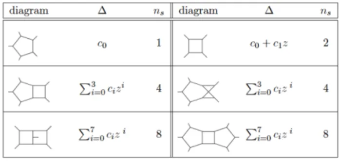
iii) A special set of on-shell cut conditions called maximum-cutsare defined by the maximum number of on-shell conditions which can be simultaneously satis- fied by the loop momenta. The Maximum Cut Theo- rem[62] ensures that their residues can always be re- constructed by evaluating the numerator at the solutions of the cut, since they are parametrized by exactlynsco- efficients, where ns is the number of solutions of the multiple cut-conditions. This theorem extends at all or- ders the features of the one-loop quadruple-cut [21, 23], where the only two complex solutions of the cut de- termine the two coefficients needed to parametrize the residue.
Figure 1: Examples of maximum-cuts.
In Figure 1, we show the structures of the residues of the maximum cut, together with the corresponding values ofns, for a selection of diagrams with different number of loops (one, two, and three). With the ex- ception of the first diagram in the left column, which represents the 5-ple cut of the 5-point one-loop dimen- sionally regulated amplitude, all the other diagrams in the table are considered in four dimensions. For each of them, the general structure of the residueΔand the cor- responding value ofnsare provided. Similar conditions can be found for more complicated topologies at higher loops.
The integrand recurrence relation of Eq. (5) can be applied in two different ways. After the parametric form of all residues has been determined, if the solutions of all multiple cuts are known, the coefficients which ap- pear in the residues can be determined by evaluating the numerator at the solutions of the multiple cuts, as many times as the number of the unknown coefficients. This approach has been employed at one loop in the original integrand reduction [23], and the language of multivari- ate polynomial division provides its generalization at all loops.
As a very different strategy [67], the decomposition can be obtained analytically by successive polynomial divisions. In this approach, the reduction algorithm is applied directly to the actual numerator functions, with- out requiring the knowledge of the parametric form of all residues or the solutions of the multiple cuts. In Ref. [67], we showed how this strategy can be success- fully applied to integrands with denominators appear- ing with multiple powers, thus solving a long-standing problem within unitarity-based methods.
4. Virtual NLO with GoSam 2.0
The idea behind the GoSamframework is to combine automated diagram generation and algebraic manipu-
lation [68–71] with the integrand-level reduction tech- niques described above. Amplitudes are automatically generated via Feynman diagrams, so that the only task required from the user is the preparation of an input file for the generation of the code, without having to worry about the internal details.
We recently released GoSam 2.0, a new version of the code that offers numerous improvements both on the generation and the reduction side, resulting in faster and more stable codes for calculations within and be- yond the Standard Model. After the generation of all contributing diagrams, the virtual corrections are eval- uated using the integrand reduction via Laurent expan- sion provided by Ninja, or thed-dimensional integrand- level reduction method, as implemented in Samurai. Alternatively, the tensorial decomposition provided by Golem95C [72, 73] is also available. GoSam2.0 can be used to generate and evaluate one-loop corrections in both QCD and electro-weak theory. Model files for Be- yond Standard Model (BSM) applications can be gener- ated from a Universal FeynRules Output (UFO) [74, 75]
or withLanHEP[76].
The code has been employed in several applications at NLO QCD accuracy [50, 51, 57, 77–81], studies of BSM scenarios [82–84], electroweak calculations [85, 86], and recently also within NNLO calculations for the production of real-virtual contributions [87–89].
GoSam2.0 also contains the extended version of the standardizedBinoth Les Houches Accord (BLHA) in- terface [90, 91] to Monte Carlo programs.
5. Production of physical results at NLO precision, interfaces with Monte Carlo tools
The computation of physical observables at NLO ac- curacy, such as cross sections and differential distri- butions, requires to combine the one-loop results for the virtual amplitudes obtained with GoSam, with other tools that can take care of the computation of the real emission contributions and of the subtraction terms, needed to control the cancellation of IR singularities.
This can be obtained by embedding the calculation of virtual corrections within a Monte Carlo framework (MC), that can provide the phase-space integration, and of the combination of the different pieces of the calcula- tion. A complete table of GoSam’s interfaces with MC programs has been recently presented in [92].
At present, the GoSam code has been successfully interfaced with several Monte Carlo tools, in order to provide insightful phenomenological applications [93–
95]. While in the following we will show exam- ples obtained within the frameworks of Sherpa [96]
and aMC@NLO [97], results have been also obtained within the Herwig++/Matchbox [98], whizard [99], and Powheg[100] frameworks.
LHC8TeV cteq6mE pdf
anti-kt: R=0.5,pT>20GeV,|η|<4.0 LO NLO
10−4 10−3 10−2
dσ/dpT,H[pb/GeV]
0 50 100 150 200 250 300 350 400
0.6 0.8 1 1.2 1.4
pT,H[GeV]
NLO/LO
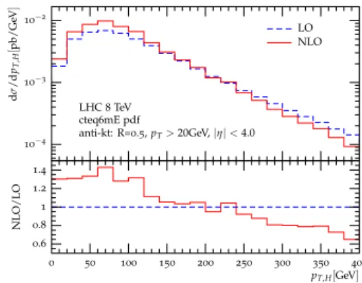
Figure 2: pp → H+3jin GF for the LHC at 8 TeV: transverse momentum distribution of the Higgs boson at LO and NLO.
Higgs boson production in Gluon Fusion. The exten- sion of integrand reduction to allow for higher rank integrands, described in Section 3.2, allowed us to compute the NLO QCD corrections to the produc- tion of H +2 jets [50] and, for the first time, also H + 3 jets [51] in Gluon Fusion in the large top- mass limit. This calculation is indeed challenging both on the side of real-emission contributions and of the virtual corrections, which alone involve more than ten thousand one-loop Feynman diagrams with up to rank-seven hexagons. Due to the complexity of the integration, for the results presented in Ref. [51]
we employed a hybrid setup which combines Go- Sam, Sherpaand the MadDipole/Madgraph4/MadEvent framework [101–105]. The pT distribution for the Higgs boson in Fig. 2 shows how the NLO correc- tions enhance all distributions forpT values lower than 150−200 GeV, whereas their contribution is negative at higherpT.
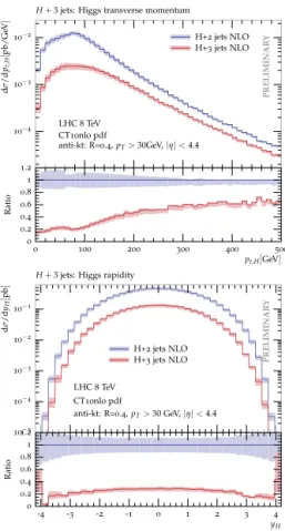
An updated analysis appeared in the “Physics at TeV Colliders: Standard Model Working Group Re- port” [12], which contains new results and distributions forH+3 jets at NLO for a set of ATLAS-like cuts and a comparison with the NLO predictions for H+2 jets (see Fig. 3), including the three-to-two jet cross section ratio at LO and NLO. Further studies for Higgs plus jets production are currently in progress, which contain the analysis of the effects of different cuts, merging with smaller multiplicities, and matching with parton shower.
LHC8TeV CT10nlo pdf
anti-kt: R=0.4,pT>30GeV,|η|<4.4
PRELIMINARY
H+2jets NLO H+3jets NLO
10−4 10−3 10−2
H+3 jets: Higgs transverse momentum
dσ/dpt,H[pb/GeV]
0 100 200 300 400 500
0 0.2 0.4 0.6 0.8 1 1.2
pt,H[GeV]
Ratio
LHC8TeV CT10nlo pdf
anti-kt: R=0.4,pT>30 GeV,|η|<4.4
PRELIMINARY
H+2jets NLO H+3jets NLO
10−5 10−4 10−3 10−2 10−1
H+3 jets: Higgs rapidity
dσ/dyH[pb]
-4 -3 -2 -1 0 1 2 3 4
0 0.2 0.4 0.6 0.8 1 1.2
yH
Ratio
Figure 3:pp→H+3jin GF for the LHC at 8 TeV: distributions of NLO transverse momentum and rapidity of the Higgs boson compared with the NLO prediction forpp→H+2j.
NLO QCD corrections to pp → t¯tH j. The production rate for a Higgs boson associated with a top-antitop pair is particularly interesting to study the coupling of the Higgs boson to the top quark. In Ref. [57], we pre- sented the calculation of the complete NLO QCD cor- rections to the process pp → t¯tH+1 jet at the LHC, which is important for the phenomenological analyses at the LHC, in particular for the high-pT region, where the presence of the additional jet can be relevant. As an illustration, in Fig. 4, we report the distribution of the top-pair invariant mass. This process is also chal- lenging by a technical point of view for the presence of two mass scales, Higgs boson and top quark, in addition to a high number of diagrams. Indeed, this calculation represented the first application and validation of the re- duction algorithm described in Section 3.3.
Further analyses forpp→ttH¯ +0,1 jets are currently in progress.
LHC 8 TeV CT10 pdf
anti-kt: R=0.5,pT>15 GeV,|η|<4.0 GoSam/Ninja+Sherpa
t¯tHjLOμ= 2×GAT t¯tHNLOμ= 2×GAT t¯tHjNLOμ= 2×GAT
10−6 10−5 10−4 10−3
H t¯t+ jet: transverse momentum of top-antitop system
dσ/dpT,t¯t
[pb/GeV]
0 100 200 300 400 500 600
0.6 0.8 1 1.2 1.4 1.6 1.8 2
pT,t¯t[GeV]
NLO/LO
Figure 4: Transverse momentum of the top-quark pair inpp→t¯tH j.
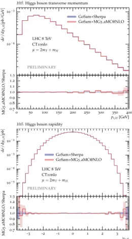
GoSam+aMC@NLOvsGoSam+Sherpa. As a last ex- ample of application of GoSam2.0, we show a compari- son between the NLO differential distributions obtained interfacing it with two different multi-purpose Monte Carlo tools. As a benchmark process, we studied the t¯tH production at the 8 TeV-LHC, with a fixed scale μ = 2mT +mH, and CT10nlo PDF set. Among the several distributions that we checked, some examples are presented in Fig. 5 and Fig. 6 . The agreement be- tween the results obtained with the two tools is remark- ably good.
A detailed work which contains a description of the interface between GoSam and aMC@NLO, together with phenomenological studies of pp → tt¯γγ, is cur- rently in progress [106].
6. Conclusions and Future Outlook
The study of scattering amplitudes provides a fertile ground for many theoretical applications. The develop- ments of the past decade show how a better understand- ing of mathematical properties of scattering amplitudes can provide the basis for the construction of efficient algorithms for their evaluation, and ultimately leads to higher quality predictions to be used in the experimen- tal analyses at the particle colliders. As of today, several different approaches available for one-loop calculations, which are encoder in different computational tools and interfaced with Monte Carlo event generators, to pro- vide NLO predictions for a variety of processes needed by the LHC experimental collaborations.
In this presentation, we reviewed the main features of the integrand reduction techniques, described some of the algorithms for the evaluation of scattering ampli- tudes that can be constructed following those ideas, and
Figure 5: Comparison GoSam+aMC@NLO vs GoSam+Sherpa, pp→ttH¯ for the LHC at 8 TeV: transverse momentum of the top quark and invariant mass of thett¯pair.
showed their application in a selection of phenomeno- logical studies for the 8 TeV-LHC, obtained within the GoSamframework.
The GoSam 2.0 release contains several improve- ments respect to its earlier versions. GoSamestablished itself as a flexible and widely applicable tool for the au- tomated calculation of the virtual part of multi-particle scattering amplitudes at NLO accuracy and provides a reliable answer for multi-leg amplitudes in the pres- ence of massive internal and external legs and propa- gators. Recent examples of calculations performed with GoSaminclude NLO QCD corrections to Higgs produc- tion channels and backgrounds, neutralino and graviton production in BSM scenarios, and electroweak correc- tions. The code has also been employed for the evalua- tion of the real-virtual part within NNLO calculations.
Several new NLO analyses are currently under way, which exploit the combination of GoSam, as provider of one-loop virtual amplitudes, within the flexible frame- work of Monte Carlo event generators. Such interfaces
LHC8TeV CT10nlo μ=2mT+mH
PRELIMINARY
GoSam+Sherpa GoSam+MG5aMC@NLO
10−4 10−3
Ht¯t: Higgs boson transverse momentum
dσ/dpt,H[pb/GeV]
0 50 100 150 200 250 300 350 400
0.7 0.8 0.9 1.0 1.1 1.2 1.3
pt,H[GeV]
MG5aMC@NLO/Sherpa
LHC8TeV CT10nlo μ=2mT+mH PRELIMINARY
GoSam+Sherpa GoSam+MG5aMC@NLO
10−5 10−4 10−3 10−2
Ht¯t: Higgs boson rapidity
dσ/dyt,H[pb]
-3 -2 -1 0 1 2 3
0.7 0.8 0.9 1.0 1.1 1.2 1.3
yt,H
MG5aMC@NLO/Sherpa
Figure 6: Comparison GoSam+aMC@NLO vs GoSam+Sherpa, pp→ttH¯ for the LHC at 8 TeV: transverse momentum of the Higgs boson, and Higgs boson rapidity.
should be improved and simplified, to allow for an au- tomated generation of analyses which include parton shower effect and the merging of different multiplicities, as needed by comparisons with experimental data.
Looking ahead, as the focus is shifting towards the challenges presented by NNLO calculations, new ideas and techniques [107–111], along with improved version of known algorithms, are starting to make an impact. In this context, it will be interesting to observe whether the extensions of integrand-level techniques to higher or- ders will succeed to provide a comparable level of reli- ability, and eventually of automation, as in the one-loop case, and to what extent the GoSamframework could be extended to explore the new frontiers in precision cal- culations.
Acknowledgments. We would like to thank the present and former members of the GoSam Collaboration for their contributions to the results presented in this talk.
H.v.D., G.L., and P.M. are supported by the Alexan-
der von Humboldt Foundation, in the framework of the Sofja Kovaleskaja Award Project Advanced Mathemat- ical Methods for Particle Physics, endowed by the Ger- man Federal Ministry of Education and Research. The work of G.O. and Z.Z. was supported in part by the Na- tional Science Foundation under Grant PHY-1068550 and PSC-CUNY Award No. 65188-00 43. G.O. also acknowledges the support of NSF under Grant PHY- 1417354. The authors are grateful to the Center for Theoretical Physics of New York City College of Tech- nology for providing computational resources.
References
[1] Englert F and Brout R 1964Phys.Rev.Lett.13321–323 [2] Higgs P W 1964Phys.Lett.12132–133
[3] Aad Get al.(ATLAS Collaboration) 2012Phys.Lett.B7161–
29 (Preprint1207.7214)
[4] Chatrchyan Set al.(CMS Collaboration) 2012Phys.Lett.B716 30–61 (Preprint1207.7235)
[5] Cullen G, Greiner N, Heinrich G, Luisoni G, Mastrolia Pet al.
2012Eur.Phys.J.C721889 (Preprint1111.2034)
[6] Cullen G, van Deurzen H, Greiner N, Heinrich G, Luisoni G et al.2014Eur.Phys.J.C743001 (Preprint1404.7096) [7] Mastrolia PPlenary Talk at SILAFAE X, in these proceedings [8] Bern Z, Dixon L J and Kosower D A 2007Annals Phys.322
1587–1634 (Preprint0704.2798)
[9] Ellis R K, Kunszt Z, Melnikov K and Zanderighi G 2012 Phys.Rept.518141–250 (Preprint1105.4319)
[10] Ossola G 2014 J.Phys.Conf.Ser. 523 012040 (Preprint 1310.3214)
[11] Heinemeyer Set al.(The LHC Higgs Cross Section Working Group) 2013 (Preprint1307.1347)
[12] Butterworth J, Dissertori G, Dittmaier S, de Florian D, Glover Net al.2014 (Preprint1405.1067)
[13] Passarino G and Veltman M J G 1979Nucl. Phys.B160151 [14] ’t Hooft G and Veltman M 1979Nucl.Phys.B153365–401 [15] van Oldenborgh G 1991Comput.Phys.Commun.661–15 [16] Hahn T and Perez-Victoria M 1999 Comput.Phys.Commun.
118153–165 (Preprinthep-ph/9807565)
[17] Ellis R K and Zanderighi G 2008 JHEP02 002 (Preprint 0712.1851)
[18] van Hameren A 2011Comput.Phys.Commun.1822427–2438 (Preprint1007.4716)
[19] Cullen G, Guillet J, Heinrich G, Kleinschmidt T, Pilon E et al.2011Comput.Phys.Commun.1822276–2284 (Preprint 1101.5595)
[20] Bern Z, Dixon L J, Dunbar D C and Kosower D A 1994Nucl.
Phys.B425217–260 (Preprinthep-ph/9403226)
[21] Britto R, Cachazo F and Feng B 2005Nucl. Phys.B725275–
305 (Preprinthep-th/0412103)
[22] del Aguila F and Pittau R 2004 JHEP0407017 (Preprint hep-ph/0404120)
[23] Ossola G, Papadopoulos C G and Pittau R 2007Nucl.Phys.
B763147–169 (Preprinthep-ph/0609007)
[24] Ossola G, Papadopoulos C G and Pittau R 2007JHEP0707 085 (Preprint0704.1271)
[25] Ossola G, Papadopoulos C G and Pittau R 2008JHEP0805 004 (Preprint0802.1876)
[26] Draggiotis P, Garzelli M, Papadopoulos C and Pittau R 2009 JHEP0904072 (Preprint0903.0356)
[27] Garzelli M, Malamos I and Pittau R 2011JHEP1101029 (Preprint1009.4302)
[28] Garzelli M and Malamos I 2011 Eur.Phys.J. C71 1605 (Preprint1010.1248)
[29] Page B and Pittau R 2013 JHEP 1309 078 (Preprint 1307.6142)
[30] Fazio R A, Mastrolia P, Mirabella E and Torres Bobadilla W J 2014Eur.Phys.J.C743197 (Preprint1404.4783)
[31] Torres Bobadilla W JPresentation at SILAFAE X, in these pro- ceedings
[32] Ossola G, Papadopoulos C G and Pittau R 2008JHEP03042 (Preprint0711.3596)
[33] Binoth T, Ossola G, Papadopoulos C and Pittau R 2008JHEP 0806082 (Preprint0804.0350)
[34] Actis S, Mastrolia P and Ossola G 2010Phys.Lett.B682419–
427 (Preprint0909.1750)
[35] Hahn T 2008PoSACAT08121 (Preprint0901.1528) [36] Bevilacqua G, Czakon M, Garzelli M, van Hameren A, Kardos
Aet al.2013Comput.Phys.Commun.184986–997 (Preprint 1110.1499)
[37] Hirschi V, Frederix R, Frixione S, Garzelli M V, Maltoni F et al.2011JHEP1105044 (Preprint1103.0621)
[38] Ellis R K, Giele W T and Kunszt Z 2008 JHEP 03 003 (Preprint0708.2398)
[39] Giele W T, Kunszt Z and Melnikov K 2008JHEP0804049 (Preprint0801.2237)
[40] Ellis R, Giele W T, Kunszt Z and Melnikov K 2009Nucl.Phys.
B822270–282 (Preprint0806.3467)
[41] Giele W and Zanderighi G 2008JHEP0806038 (Preprint 0805.2152)
[42] Pittau R 1997Comput. Phys. Commun.10423–36 (Preprint hep-ph/9607309)
[43] Bern Z and Morgan A G 1996Nucl. Phys. B467479–509 (Preprinthep-ph/9511336)
[44] Mastrolia P, Ossola G, Reiter T and Tramontano F 2010JHEP 1008080 (Preprint1006.0710)
[45] Melnikov K and Schulze M 2010Nucl.Phys.B840129–159 (Preprint1004.3284)
[46] Mastrolia P, Ossola G, Papadopoulos C and Pittau R 2008 JHEP0806030 (Preprint0803.3964)
[47] Agrawal S, Hahn T and Mirabella E 2012J.Phys.Conf.Ser.368 012054 (Preprint1112.0124)
[48] Nejad B C, Hahn T, Lang J N and Mirabella E 2013 (Preprint 1310.0274)
[49] Cascioli F, Maierhofer P and Pozzorini S 2012Phys.Rev.Lett.
108111601 (Preprint1111.5206)
[50] van Deurzen H, Greiner N, Luisoni G, Mastrolia P, Mirabella Eet al.2013Phys.Lett.B72174–81 (Preprint1301.0493) [51] Cullen G, van Deurzen H, Greiner N, Luisoni G, Mastrolia P
et al.2013Phys.Rev.Lett.111131801 (Preprint1307.4737) [52] Mastrolia P, Mirabella E, Ossola G, Peraro T and van Deurzen
H 2012PoSLL2012028 (Preprint1209.5678)
[53] Mastrolia P, Mirabella E and Peraro T 2012JHEP1206095 (Preprint1203.0291)
[54] van Deurzen H 2013Acta Phys.Polon.B442223–2230 [55] Peraro T 2014 Comput.Phys.Commun. 185 2771–2797
(Preprint1403.1229)
[56] van Deurzen H, Luisoni G, Mastrolia P, Mirabella E, Ossola G et al.2014JHEP1403115 (Preprint1312.6678)
[57] van Deurzen H, Luisoni G, Mastrolia P, Mirabella E, Ossola G et al.2013Phys.Rev.Lett.111171801 (Preprint1307.8437) [58] Gro C, Hahn T, Heinemeyer S, von der Pahlen F, Rzehak H
et al.2014 (Preprint1407.0235)
[59] Mastrolia P and Ossola G 2011JHEP1111014 (Preprint 1107.6041)
[60] Badger S, Frellesvig H and Zhang Y 2012JHEP1204055 (Preprint1202.2019)
[61] Zhang Y 2012JHEP1209042 (Preprint1205.5707) [62] Mastrolia P, Mirabella E, Ossola G and Peraro T 2012
Phys.Lett.B718173–177 (Preprint1205.7087)
[63] Kleiss R H, Malamos I, Papadopoulos C G and Verheyen R 2012JHEP1212038 (Preprint1206.4180)
[64] Badger S, Frellesvig H and Zhang Y 2012JHEP1208065 (Preprint1207.2976)
[65] Feng B and Huang R 2013 JHEP 1302 117 (Preprint 1209.3747)
[66] Mastrolia P, Mirabella E, Ossola G and Peraro T 2013 Phys.Rev.D87085026 (Preprint1209.4319)
[67] Mastrolia P, Mirabella E, Ossola G and Peraro T 2013 Phys.Lett.B727532–535 (Preprint1307.5832)
[68] Nogueira P 1993J.Comput.Phys.105279–289 [69] Vermaseren J A M 2000 (Preprintmath-ph/0010025) [70] Reiter T 2010 Comput.Phys.Commun. 181 1301–1331
(Preprint0907.3714)
[71] Cullen G, Koch-Janusz M and Reiter T 2011 Com- put.Phys.Commun.1822368–2387 (Preprint1008.0803) [72] Binoth T, Guillet J P, Heinrich G, Pilon E and Reiter
T 2009 Comput.Phys.Commun. 180 2317–2330 (Preprint 0810.0992)
[73] Heinrich G, Ossola G, Reiter T and Tramontano F 2010JHEP 1010105 (Preprint1008.2441)
[74] Degrande C, Duhr C, Fuks B, Grellscheid D, Mattelaer O et al.2012Comput.Phys.Commun.1831201–1214 (Preprint 1108.2040)
[75] Alloul A, Christensen N D, Degrande C, Duhr C and Fuks B 2014 Comput.Phys.Commun. 185 2250–2300 (Preprint 1310.1921)
[76] Semenov A 2014 (Preprint1412.5016)
[77] Greiner N, Guffanti A, Reiter T and Reuter J 2011 Phys.Rev.Lett.107102002 (Preprint1105.3624)
[78] Greiner N, Heinrich G, Mastrolia P, Ossola G, Reiter Tet al.
2012Phys.Lett.B713277–283 (Preprint1202.6004) [79] Gehrmann T, Greiner N and Heinrich G 2013JHEP1306058
(Preprint1303.0824)
[80] Gehrmann T, Greiner N and Heinrich G 2013 (Preprint 1308.3660)
[81] Dolan M J, Englert C, Greiner N and Spannowsky M 2013 (Preprint1310.1084)
[82] Cullen G, Greiner N and Heinrich G 2013Eur.Phys.J.C73 2388 (Preprint1212.5154)
[83] Greiner N, Heinrich G, Reichel J and von Soden-Fraunhofen J F 2013JHEP1311028 (Preprint1308.2194)
[84] Greiner N, Kong K, Park J C, Park S C and Winter J C 2014 (Preprint1410.6099)
[85] Chiesa M, Montagna G, Barze‘ L, Moretti M, Nicrosini Oet al.
2013Phys.Rev.Lett.111121801 (Preprint1305.6837) [86] Mishra K, Becher T, Barze L, Chiesa M, Dittmaier Set al.2013
(Preprint1308.1430)
[87] Gao J and Zhu H X 2014Phys.Rev.D90114022 (Preprint 1408.5150)
[88] Gao J and Zhu H X 2014Phys.Rev.Lett.113262001 (Preprint 1410.3165)
[89] Del Duca V, Duhr C, Somogyi G, Tramontano F and Trocsanyi Z 2015 (Preprint1501.07226)
[90] Binoth T, Boudjema F, Dissertori G, Lazopoulos A, Denner A et al.2010Comput.Phys.Commun.1811612–1622 (Preprint 1001.1307)
[91] Alioli S, Badger S, Bellm J, Biedermann B, Boudjema Fet al.
2013 (Preprint1308.3462)
[92] van Deurzen H, Greiner N, Heinrich G, Luisoni G, Mirabella
Eet al.2014PoSLL2014021 (Preprint1407.0922) [93] Luisoni G, Nason P, Oleari C and Tramontano F 2013JHEP
1310083 (Preprint1306.2542)
[94] Hoeche S, Huang J, Luisoni G, Schoenherr M and Winter J 2013Phys.Rev.D88014040 (Preprint1306.2703)
[95] Luisoni G, Oleari C and Tramontano F 2015 (Preprint 1502.01213)
[96] Gleisberg T, Hoeche S, Krauss F, Schonherr M, Schumann S et al.2009JHEP0902007 (Preprint0811.4622)
[97] Alwall J, Frederix R, Frixione S, Hirschi V, Maltoni Fet al.
2014JHEP1407079 (Preprint1405.0301)
[98] Bellm J, Gieseke S, Grellscheid D, Papaefstathiou A, Platzer S et al.2013 (Preprint1310.6877)
[99] Reuter J, Bach F, Chokoufe B, Kilian W, Ohl Tet al.2014 (Preprint1410.4505)
[100] Alioli S, Nason P, Oleari C and Re E 2010JHEP1006043 (Preprint1002.2581)
[101] Frederix R, Gehrmann T and Greiner N 2008JHEP0809122 (Preprint0808.2128)
[102] Frederix R, Gehrmann T and Greiner N 2010JHEP1006086 (Preprint1004.2905)
[103] Stelzer T and Long W 1994Comput.Phys.Commun.81357–
371 (Preprinthep-ph/9401258)
[104] Maltoni F and Stelzer T 2003 JHEP 0302 027 (Preprint hep-ph/0208156)
[105] Alwall J, Demin P, de Visscher S, Frederix R, Herquet Met al.
2007JHEP0709028 (Preprint0706.2334)
[106] van Deurzen H, Frederix R, Hirschi V, Luisoni G, Mastrolia P and Ossola GIn preparation
[107] Henn J M 2013 Phys.Rev.Lett. 110 251601 (Preprint 1304.1806)
[108] Argeri M, Di Vita S, Mastrolia P, Mirabella E, Schlenk Jet al.
2014JHEP1403082 (Preprint1401.2979)
[109] Papadopoulos C G 2014 JHEP 1407 088 (Preprint 1401.6057)
[110] Gehrmann T, von Manteuffel A, Tancredi L and Weihs E 2014 JHEP1406032 (Preprint1404.4853)
[111] Lee R N 2014 (Preprint1411.0911)