Optimization Despite Chaos:
Convex Relaxations to Complex Limit Sets via Poincar´e Recurrence
Georgios Piliouras ∗
School of Electrical and Computer Engineering Georgia Institute of Technology
Jeff S. Shamma
School of Electrical and Computer Engineering Georgia Institute of Techonology
Abstract
It is well understood that decentralized systems can, through network interactions, give rise to complex be- havior patterns that do not reflect their equilibrium properties. The challenge of any analytic investigation is to identify and characterize persistent properties de- spite the inherent irregularities of such systems and to do so efficiently. We develop a novel framework to ad- dress this challenge.
Our setting focuses on evolutionary dynamics in network extensions of zero-sum games. Such dynam- ics have been shown analytically to exhibit chaotic be- havior which traditionally has been thought of as an overwhelming obstacle to algorithmic inquiry. We cir- cumvent these issues as follows: First, we combine ideas from dynamical systems and game theory to pro- duce topological characterizations of system trajecto- ries. Trajectories capture the time evolution of the sys- tem given an initial starting state. They are complex, and do not necessarily converge to limit points or even limit cycles. We provide tractable approximations of such limit sets. These relaxed descriptions involve sim- plices, and can be computed in polynomial time. Next, we apply standard optimization techniques to compute extremal values of system features (e.g. expected util- ity of an agent) within these relaxations. Finally, we use information theoretic conservation laws along with Poincar´ e recurrence theory to argue about tightness and optimality of our relaxation techniques.
∗
This work is supported by FA9550-09-1-0538. Authors’ ad- dresses: G. Piliouras, School of Electrical and Computer Engi- neering, Georgia Institute of Technology, georgios@gatech.edu;
J.S. Shamma, School of Electrical and Computer Engineering, Georgia Institute of Technology, shamma@gatech.edu.
1 Introduction
Complex networks are increasingly integrated in the very fabric of our society. As much as these networks bring people together and facilitate cooperation, they also give rise to unexpected behavior patterns. Over the last decade, the prevalence of such issues has risen dramatically following a number of paradigm-shifting events such as the meteoric rise of the Internet as a social networking tool, the painful realization of the extent of inter-connectivity of the global economy as well as the necessity of international cooperation for addressing global sustainability concerns.
Within computer science, algorithmic game theory has been developed in an effort to provide a quantita- tive lens for studying such systems. With classic game theory as a guiding beacon, Nash equilibrium analysis quickly became the de facto solution standard. Despite its prominent role, this direction has been the subject of much criticism. In games with multiple equilibria, it is unclear how agents are expected to coordinate on one. Furthermore, identifying a single Nash equilibrium may involve unreasonable expectations on agent com- munication and computation. Finally, natural adaptive play does not converge to Nash equilibria in general games. In fact, there exist games with constant number of agents and strategies in which natural learning dy- namics converge to limit cycles of optimal social welfare which can be arbitrarily better than the social welfare of the best equilibrum [23, 25].
Equilibrium analysis has emerged pretty much un- scathed from these remarks. To counter this disconnect between the proposed equilibrium methodology and the usually more intricate system behavior, proponents of the equilibrium approach rightfully point out that equi- librium analysis already raises significant analytical hur- dles. Once we move past the safe haven of Nash equi-
Downloaded 12/04/21 to 118.70.52.165 Redistribution subject to SIAM license or copyright; see https://epubs.siam.org/page/terms
libria, which capture (possibly unstable) fixed points of learning dynamics, the topological waters become deep and turbulent fast. Indeed, in [29] Sato etal. make this argument rather convincingly by showing that even sim- ple zero-sum games (perturbed versions of Rock-Paper- Scissors) suffice to give rise to chaotic behavior under classic evolutionary dynamics. Specifically, they an- alytically verify high sensitivity of system trajectories to initial conditions and provide experimental evidence of dense interweaving between quasi-periodic tori and chaotic orbits.
A cursory glance at the rate of progress of theoret- ical work on disequilibrium dynamics is rather telling about the complexities involved. Soon after Nash for- malized his ideas about equilibrium, Shapley [31] es- tablished that simple learning dynamics do not con- verge to equilibrium. The game in question is a two agent non-zero sum variant of Rock-Paper-Scissors. Fol- lowup work by Jordan[21] established analogous results for three agent games. These results have been revis- ited and reestablished via different routes [14]. Within computer science recent work about non-convergence of learning dynamics in games focuses on variants of these games and dynamics [8, 23, 3]. The unified characteris- tics of all these works, which are already present in the work of Shapley, are that the networks are of constant size, the dimension of the action space is constant, and that the disequilibrium behavior is as simple as possi- ble. Specifically, the dynamics exhibit a single polygon- shaped cyclic attractor with a constant number of ver- tices. These attractors are usually referred to as Shapley polygons.
Another key common characteristic of this prior work is that it is largely qualitative in nature. The goal is to present a simple and easy to convey message.
Given that chaotic phenomena can arise even in simple examples, researchers traverse a fine line of identifying classes of games whose hardness is exactly right. The settings must be simple enough so that the true system behavior can be expressed concisely and with perfect precision, and rich enough so that the resulting picture diverges significantly from that of standard equilibrium analysis.
Such approaches are undoubtedly useful in terms of cultivating a collective mindset about the importance of meeting these analytical challenges fully. However, if nonequilibrium analysis hopes to graduate to the level of a concrete and actionable scientific framework one needs to show how progress in this area can translate to novel algorithmic insights. How can one compute, or even efficiently encode, regularities in an ever transient complex environment? We hope to shed some light along this direction.
Our results We study an evolutionary class of dynam- ics, the replicator equation, in a network generaliza- tion of constant-sum games known as separable zero- sum multiplayer games. These are polymatrix graphi- cal games where the sum of all agents’ payoffs is always equal to zero. This setting incorporates both the com- plexity of chaotic trajectories as well as computational intricacies that arise from its combinatorial structure.
Specifically, we present the first to our knowledge anal- ysis of nonequilibrium dynamics for a class of games of arbitrary dimension (number of agents, number of strategies).
We introduce formal notions of persistent properties for nonconverging dynamics. Roughly speaking, a sub- space of the state space defines a persistent property if for all initial conditions systems trajectories eventually move away from the complement of the subspace and never return to it. Arguing about persistent properties requires topological characterizations of system trajec- tories. In generic (network) zero-sum games no trajec- tory converges to equilibrium. We combine elements from theory of dynamical systems, game theory and on- line learning theory to show that the limit sets of all starting points lie within a specific subspace. This sub- space is a product of simplices and expresses the set of all mixed strategy profiles whose support matches that of the Nash equilibrium of maximum support. Further- more, we utilize an information theoretic conservation law to extend Poincar´ e recurrence theory to our setting and argue about the optimality of the relaxation.
In the second part of the paper we show how we can combine these topological characterizations with algo- rithmic tools to make tight predictions about the pos- sible range of values of interesting system features. We start by extending ideas from algorithmic game theory to show that we can compute these simplex-based re- laxed descriptions efficiently. Next, we show that solv- ing optimization problems over such relaxed subsets suf- fices to track extremal recurrent value problems for con- tinuous features of the state space (e.g. expected utility of an agent). Finally, we discuss some concrete appli- cations of our framework towards identifying margins of survival as well as optimal performance measures for competing companies in networked economies.
A benchmark example: Rock-Paper-Scissors Let’s consider the benchmark case of the Rock-Paper Scissors game in order to convey some concrete insights.
A key observation is that starting from any (interior) starting point the sum of the K-L divergences between the unique fully mixed Nash equilibrium strategy of each agent and her evolving strategy remains constant as the system moves forward in time. A useful fact to keep in mind is that K-L divergence can be thought
Downloaded 12/04/21 to 118.70.52.165 Redistribution subject to SIAM license or copyright; see https://epubs.siam.org/page/terms
of as a (pseudo)-metric.
1The fact that this pseudo- distance between the Nash equilibrium and the evolving system state remains constant is useful. Intuitively, it implies that the replicator dynamics starting from a fully mixed state will: a) not converge to the Nash equilibrium (K-L divergence cannot drop to zero); b) will not come arbitrarily close to the boundary (K-L divergence cannot blow up to infinity). In fact, for any two initial conditions (mixed strategy profiles) x and y with distinct initial K-L divergences from the Nash equilibrium the corresponding limit behavior must be distinct. This richness in limit behavior (with infinitely many different possible limit behaviors) comes at a contrast with the established intuition about zero-sum games having a unique behavioral “solution”.
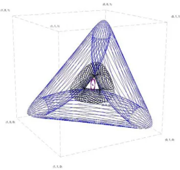
Figure 1: Sample orbits of replicator dynamics in Rock- Paper-Scissors (row agent’s mixed strategy)
More to the point, our analysis implies that given any open set of initial conditions that is bounded away from the boundary there exist replicator trajectories that revisit this set infinitely often. Before we examine how one could prove such a statement, let’s examine why such a statement is useful. Let’s imagine an outside observer that makes a measurement of a continuous observable feature
2every time this trajectory “hits” the
1
The K-L divergence between two distributions is non-negative and it is equal zero if and only if the two distributions match. It is also finite for any two distributions with the same support.
2
For now, think of a feature as a function from the state space to the real line.
open set. If we define the open set as an (open) ball of radius δ > 0, then for any ϵ > 0 we can choose such a δ > 0 such that any two such measurements are within an ϵ of each other. For all practical purposes these observations become indistinguishable for small enough ϵ, δ. Since these (range of) values can be revisited infinitely often (for properly chosen initial conditions) a predictive statement that holds regardless of initial conditions must account for them. Using properly chosen open balls of initial conditions we can approximate any value of a continuous feature (anywhere on the state space) within an error of ϵ for any ϵ > 0. Therefore, without explicit knowledge of initial conditions, the only closed set of predictions that we can make for any continuous feature is the trivial one, i.e., the set that includes all possible range of values. So, not only is the unique Nash equilibrium not predictive of the actual day-to-day agent behavior (or any continuous observable feature of it) but from an optimization point- of-view no nontrivial prediction can be made!
This recurrence of observed values would be im- mediately true if all trajectories where either fixed points (i.e. Nash equilibria) or formed limit cycles, that is, if they looped perfectly into themselves. Un- fortunately, this concise characterization is not true even for separable zero-sum games with a unique fully mixed Nash equilibrium
3. We need to apply a more re- laxed and powerful notion of recurrence that dates back to Poincar´ e and his celebrated 1890’s memoir on the three body problem [28]. Poincar´ e’s recurrence theo- rem states that the trajectories of certain systems re- turn arbitrarily close to their initial position and that they do this an infinite number of times. Combining the fact that in Rock-Paper-Scissors given any initial fully mixed strategy the system state stays away from boundary along with other technical properties of the replicator dynamic, we show how to extend the impli- cations of this theorem to our setting and prove recur- rence of open sets. Specifically, we establish topological conjugacies, which is a powerful notion of equivalence for flows, between replicator flows and specific classes of conservative systems for which Poincar´ e’s recurrence theorem is known to apply.
Related Work Persistent cyclic or chaotic patterns are a ubiquitous reality of natural systems. Research on the intersection of mathematical ecology and dynamical systems dating back to the 70’s[10, 11, 13, 16] has developed a wide range of tools for addressing the following question: Given a dynamical system capturing
3
Such an example is a setting consisting of two independent copies of matching pennies where the utilities in one of the games have been scaled up by an irrational number.
Downloaded 12/04/21 to 118.70.52.165 Redistribution subject to SIAM license or copyright; see https://epubs.siam.org/page/terms
the interaction of different species in a population is it true that all species will survive in the long run? In our work we apply these tools towards understanding other abstract properties of our state space. More extended surveys of results in the area can be found here[20, 18].
Our work was inspired by recent insights on net- work generalizations of zero-sum games[9, 6]. Their approach is mostly focused on the properties of Nash equilibria. Nash equilibrium computation is shown to be tractable. Furthermore, the set of Nash equilibria is convex. Lastly, the time-average of no-regret dynamics converges weakly to the set of Nash equilibria. On the contrary our work focuses on the “day-to-day” prop- erties of the trajectories of the replicator dynamic, an explicit regret-minimizing dynamic.
In terms of analyzing replicator dynamics in set- tings of interest, the work of Kleinberg, Piliouras and Tardos[24] show how replicator when applied to generic potential games leads to the collapse of the randomiza- tion of an initial generic state. The story we are pre- senting here is essentially the dual of that in potential games. Replicator dynamics leads to the preservation of as much of the initial randomness of the system as pos- sible. Our tools for analyzing replicator dynamics build upon the work of Akin and Losert[1] on symmetric zero- sum games without however following in the footsteps of their symplectic forms approach. The other major influence to our work has come from the work of Hof- bauer, who amongst other contributions in the area was the first to offer formal connections between replicator dynamics and conservative systems via smooth invert- ible mappings[17, 18].
2 Preliminaries
In this section, we introduce the necessary concepts and notions that will enable us to express our points formally. Several of the concepts such as the replicator dynamic and the overview of dynamical systems theory are classic, however, other ones such as that of feature, property and persistent property are novel.
2.1 Separable zero-sum multiplayer game A graphical polymatrix game is defined via an undirected graph G = (V, E), where V corresponds to the set of agents of the game and where every edge corresponds to a bimatrix game between its two endpoints/agents.
We denote by S i the set of strategies of agent i. We de- note the bimatrix game on edge (i, k) ∈ E via a pair of payoff matrices: A i,k of dimension | S i |×| S k | and A k,i of dimension | S k | × | S i | . Let s ∈ × i S i be a strategy profile of the game. We denote by s i ∈ S i the respective strat- egy of agent i. Similarly, we denote by s
−i ∈ × j
∈V
\i S j
the strategies of the other agents. The payoff of agent
i ∈ V in strategy profile s is equal to the sum of the pay- offs that agent i receives from all the bimatrix games she participates in. Specifically, u i (s) = ∑
(i,k)∈
E A i,k s
i,s
k. A randomized strategy x for agent i lies on the simplex ∆(S i ) = { p ∈
|+S
i|: ∑
i p i = 1 } . A randomized strategy x is said to be fully mixed if it lies in the interior of the simplex, i.e. if x i > 0 for all strategies i ∈ S i . Payoff functions are extended to randomized strategies in the usual multilinear fashion. A (mixed) Nash equilibrium is a profile of mixed strategies such that no agent can improve her (expected) payoff by unilaterally deviating to another strategy.
Definition 2.1. (Separable zero-sum multiplayer games) [6] A separable zero-sum multiplayer game GG is a graphical polymatrix game in which, for any pure strategy profile, the sum of all players’ payoffs is zero.
Formally, ∀ s ∈ × i S i , ∑
i u i (s) = 0.
Zero-sum games trivially have this property. Any graphical games in which every edge is a zero-sum game also belongs to this class. These games are referred to as pairwise zero-sum polymatrix games [9]. If the edges are allowed to be arbitrary constant-sum games then the corresponding games are called pairwise constant-sum polymatrix games. There exists [6] a (polynomial-time computable) payoff preserving transformation from ev- ery separable zero-sum multiplayer game to a pairwise constant-sum polymatrix game (i.e., a game played on a graph with agents on the nodes and two-agent games on each edge such for each i, k ∈ V : A k,i = c
{k,i
}1 − A
Ti,k and 1 the all-one matrix). We will use this representa- tion in the rest of the paper.
2.2 Replicator Dynamics The replicator equation is among the basic tools in mathematical ecology, genet- ics, and mathematical theory of selection and evolution.
In its classic continuous form, it is described by the fol- lowing differential equation:
˙
x i , dx i (t)
dt = x i [u i (x) − u(x)], ˆ u(x) = ˆ
∑ n
i=1
x i u i (x) where x i is the proportion of type i in the population, x = (x
1, . . . , x m ) is the vector of the distribution of types in the population, u i (x) is the fitness of type i, and ˆ u(x) is the average population fitness. The state vector x can also be interpreted as a randomized strategy of an adaptive agent that learns to optimize over its m possible actions given an online stream of payoff vectors. The right hand-size of the replicator equation defines a continuously differentiable function defined on (the interior) of the associated simplex. This
Downloaded 12/04/21 to 118.70.52.165 Redistribution subject to SIAM license or copyright; see https://epubs.siam.org/page/terms
function is referred to as the vector field ξ. Since the replicator allows to associate stream of payoff vectors to mixed strategies, it can be employed in any distributed optimization setting by having each agent update her strategy according to it. A fixed point of the replicator is a point where its vector field is equal to the zero vector.
Such points are stationary, i.e., if the system starts off from such a point it stays there. An interior point of the state space is a fixed point for the replicator if and only if it is a fully mixed Nash equilibrium of the game. The interior (the boundary) of the state space × i ∆(S i ) are invariants for the replicator. We typically analyze the behavior of the replicator from a generic interior point, since points of the boundary can be captured as interior points of lower dimensional systems. Summing all this up, our model is captured by the following system:
˙
x iR = x iR (
u i (R) − ∑
R
′∈S
ix iR
′u i (R
′) )
for each agent i ∈ N , action R ∈ S i , and where we define u i (R) = E s
−i∼x
−iu i (R, s
−i ).
The replicator dynamic enjoys numerous desirable properties such as universal consistency (no-regret)[12, 19], connections to the principle of minimum discrimi- nation information (Occam’s rajor, Bayesian updating), disequilibrium thermodynamics[22, 30], classic models of ecological growth (e.g. Lotka-Volterra equations[18]), as well as several well studied discrete time learning al- gorithms (e.g. Multiplicative Weights algorithm[24, 2]).
2.3 Topology of dynamical systems In an effort to make our work as standalone as possible we provide a quick introduction to the main ideas in the topology of dynamical systems. Our treatment follows that of [32], the standard text in evolutionary game theory, which itself borrows material from the classic book by Bhatia and Szeg¨ o[5].
Since our state space is compact and the replicator vector field is Lipschitz-continuous, we can present the unique solution of our ordinary differential equation as a continuous map Φ : S × → S called flow of the system. Fixing starting point x ∈ S defines a function of time which captures the trajectory (orbit, solution path) of the system with the given starting point. This corresponds to the graph of Φ(x, · ) : → S , i.e., the set { (t, y) : y = Φ(x, t) for some t ∈ } . In simple terms, the trajectory captures the evolution of the state of a system given an initial starting point. On the other hand, by fixing time t, we obtain a map of the state space to itself Φ t : S → S . The resulting family of mappings exhibits the standard group properties such as identity (Φ
0) and existence of inverse (Φ
−t ), and closure under composition Φ t
1◦ Φ t
2= Φ t
1+t2.
If the starting point x does not correspond to an equilibrium, then we wish to capture the asymptotic behavior of the system (informally the limit of Φ(x, t) when t goes to infinity). Typically, however, such functions do not exhibit a unique limit point so instead we study the set of limits of all possible convergent subsequences. Formally, given a dynamical system (, S , Φ) with flow Φ : S × → S and a starting point x ∈ S , we call point y ∈ S an ω-limit point of the orbit through x if there exists a sequence (t n ) n
∈N∈ such that lim n
→∞t n = ∞ , lim n
→∞Φ(x, t n ) = y.
Alternatively the ω-limit set can be defined as: ω
Φ(x) =
∩ t ∪ τ
≥t Φ(x, τ).
Finally, the boundary of a subset S is the set of points in the closure of S, not belonging to the interior of S. Generally, given a subset S of a metric space with metric dist, then x is an interior point of S if there exists r > 0, such that y is in S whenever the dist(x, y) < r.
In the typical case of a Euclidean space, then simply x is an interior point if there exists an open set centered at it which is contained in S . An element of the boundary of S is called a boundary point of S. We denote the boundary of a set S as bd(S) and the interior of S as int(S). In the case of the replicator dynamics where the state space S corresponds to a product of agent (mixed) strategies we will denote by Φ i (x, t) the projection of the state on the simplex of mixed strategies of agent i.
Liouville’s Formula Liouville’s formula can be ap- plied to any system of autonomous differential equa- tions with a continuously differentiable vector field ξ on an open domain of S ⊂ k . The divergence of ξ at x ∈ S is defined as the trace of the corresponding Jacobian at x, i.e., div[ξ(x)] = ∑ k
i=1
∂ξ
i∂x
i(x). Since di- vergence is a continuous function we can compute its integral over measurable sets A ⊂ S . Given any such set A, let A(t) = { Φ(x
0, t) : x
0∈ A } be the image of A under map Φ at time t. A(t) is measurable and is vol- ume is vol[A(t)] = ∫
A(t) dx. Liouville’s formula states that the time derivative of the volume A(t) exists and is equal to the integral of the divergence over A(t):
d
dt [A(t)] =
∫
A(t)
div[ξ(x)]dx.
A vector field is called divergence free if its diver- gence is zero everywhere. Liouville’s formula trivially implies that volume is preserved in such flows.
Poincar´ e’s recurrence theorem The notion of re- currence that we will be using in this paper goes back to Poincar´ e and specifically to his study of the three- body problem. In 1890, in his celebrated work[28], he proved that whenever a dynamical system preserves vol-
Downloaded 12/04/21 to 118.70.52.165 Redistribution subject to SIAM license or copyright; see https://epubs.siam.org/page/terms
ume almost all trajectories return arbitrarily close to their initial position, and they do so an infinite num- ber of times. More precisely, Poincar´ e established the following:
Theorem 2.1. [28, 4] If a flow preserves volume and has only bounded orbits then for each open set there exist orbits that intersect the set infinitely often.
Homeomorphisms, Diffeomorphisms and Conju- gacy of Flows A function f between two topological spaces is called a homeomorphism if it has the following properties: f is a bijection, f is continuous, and f has a continuous inverse. A function f between two topo- logical spaces is called a diffeomorphism if it has the following properties: f is a bijection, f is continuously differentiable, and f has a continuously differentiable inverse.
Definition 2.2. (Topological conjugacy) Two flows Φ t : A → A and Ψ t : B → B are conjugate if there exists a homeomorphism g : A → B such that for each x ∈ A and t ∈ :
g(Φ t (x)) = Ψ t (g(x)).
Furthermore, two flows Φ t : A → A and Ψ t : B → B are diffeomorhpic if there exists a diffeomorphism g : A → B such that for each x ∈ A and t ∈ g(Φ t (x)) = Ψ t (g(x)). If two flows are diffeomorphic, then their vector fields are related by the derivative of the conjugacy. That is, we get precisely the same result that we would have obtained if we simply transformed the coordinates in their differential equations [26].
2.4 Feature and Property Generally, let Σ denote a system with a state space S whose temporal evolution is captured by the flow Φ : S × → S . We define an (observable) feature of Σ as a map F : S → O from S to (a possibly different) observation space O. For our system, where S corresponds to the product of mixed strategies of the agents × i ∆(S i ), typical examples of observable features are the (mixed) strategy or the (expected) utility of an agent.
The temporal evolution of system Σ induces orbits on the observation space Ψ = F ◦ Φ : S × → O that encode all possible systematic interactions between the system and the F -observer. A systematic analysis of feature F in Σ now translates to identifying regularities over all possible orbits of Ψ. Given feature F : S → O, we will denote as property Γ ⊂ O an open subset
4that encodes a desirable parameter range for that specific feature.
4
We will assume that all spaces including O are compact metric spaces.
2.5 Persistence The notions of persistence that we pursue here are inspired by more restricted notions of population persistence developed within the field of mathematical ecology[[18, 20] and references therein].
Definition 2.3. Given feature F : S → O, let property Γ ⊂ O be an open subset that encodes a desirable feature range. We state that property Γ is persistent for feature F if for all initial conditions x ∈ int( S ),we have that
lim inf
t
→∞dist( F ( Φ(x, t) )
, O \ Γ) > 0.
Furthermore, if ∃ ϵ > 0 such that ∀ x ∈ int( S ),we have that
lim inf
t
→∞dist( F ( Φ(x, t) )
, O \ Γ) > ϵ
then we state that property Γ is uniformly persistent for feature F .
These notions encode self-enforcing system regular- ities. That is, regardless of the starting state of the system, even if we start from states that do not satisfy a persistent property, such properties will eventually be- come true for the system and persist being true for all time. The typical way of enforcing regularities of simi- lar form in a multi-agent system is to assume that the system state will converge to (a subset of) Nash equilib- ria and show that this property is satisfied for all such limit points. However, the notion of persistence prop- erty is stronger than these statements. For example, a property that is only true exactly at a Nash equilib- rium may never be satisfied even if the system converges asymptotically to the equilibrium. On the contrary, a persistent property will eventually be satisfied. The def- inition of uniform persistence is even stronger and es- sentially states that the persistence of the property can be verified even via measurements of finite accuracy.
The are two observation spaces O of particular importance. One is the state space itself S in the case where F is the identity function. In this case, by identifying persistent properties Γ ⊂ S we essentially gain information about the topology of the ω-limit points of system trajectories. Nash equilibria trivially belong to this set for all dynamics that are Nash stationary (as the replicator). However, as we will see these sets can be significantly larger.
The other special case is when the observation space O is the real line . This is of particu- lar importance because it allows us to forge con- nections to standard optimization theory. In this case, we will simply say that F is [m,M]-persistent if we have that: inf x
∈int(S)lim inf t
→∞F (
Φ(x, t) )
≥ m and sup x
∈int(S)lim sup t
→∞F (
Φ(x, t) )
≤ M.
Downloaded 12/04/21 to 118.70.52.165 Redistribution subject to SIAM license or copyright; see https://epubs.siam.org/page/terms
2.6 Information Theory Entropy is a measure of the uncertainty of a random variable and captures the expected information value from a measurement of the random variable. The entropy H of a discrete random variable X with possible values { 1, . . . , n } and probability mass function p(X ) is defined as H(X ) =
− ∑ n
i=1 p(i) ln p(i).
Given two probability distributions p and q of a discrete random variable their K-L divergence (relative entropy) is defined as D
KL(p ∥ q) = ∑
i ln ( p(i)
q(i)
) p(i).
It is the average of the logarithmic difference between the probabilities p and q, where the average is taken using the probabilities p. The K-L divergence is only defined if q(i) = 0 implies p(i) = 0 for all i
5. K-L divergence is a ”pseudo-metric” in the sense that for it is always non-negative and is equal to zero if and only if the two distributions are equal (almost everywhere).
Other useful properties of the K-L divergence is that it is additive for independent distributions and that it is jointly convex in both of its arguments; that is, if (p
1, q
1) and (p
2, q
2) are two pairs of distributions then for any 0 ≤ λ ≤ 1: D
KL(λp
1+ (1 − λ)p
2∥ λq
1+ (1 − λ)q
2) ≤ λD
KL(p
1, q
1) + (1 − λ)D
KL(p
2, q
2).
A closely related concept is that of the cross entropy between two probability distributions, which measures the average number of bits needed to identify an event from a set of possibilities, if a coding scheme is used based on a given probability distribution q, rather than the “true” distribution p. Formally, the cross entropy for two distributions p and q over the same probability space is defined as follows: H (p, q) =
− ∑ n
i=1 p(i) ln q(i) = H(p) + D
KL(p ∥ q). For more details and proofs of these basic facts the reader should refer to the classic text by Cover and Thomas [7].
3 Topology of Persistence Properties
We will start our analysis by examining the set of (uniformly) persistent properties of system trajecto- ries. Here, we will assume that the observer F has full access to the realized state of the system at each time instance. In other words, the observation func- tion F , defined on the state space of mixed strategy outcomes × i ∆(S i ), is the identity function. Specifi- cally, the existence of any uniformly persistent prop- erty implies at a minimum: ∃ ϵ > 0 such that ∀ x ∈ int( × i ∆(S i )):lim inf dist(Φ(x, t), bd( × i ∆(S i ))) > ϵ.
To simplify notation, when the analysis of the orbit Φ(x
0, t), does not dependent critically on the initial starting point x
0, we will denote the state at time t, as x(t) or simply x.
5
The quantity 0 ln 0 is interpreted as zero because lim
x→0x ln(x) = 0.
Theorem 3.1. Let Φ denote the flow of the replicator dynamic when applied to a network-zero-sum game and let the observation function F be the identity function.
If × i int(∆(S i )) is a uniformly persistent property of the flow then the flow has a unique interior fixed point q.
Proof. If × i int(∆(S i )) is a uniformly persistent prop- erty of the flow, then by definition ∃ ϵ > 0 such that
∀ x ∈ int( × i ∆(S i )) lim inf dist(Φ(x, t), bd( × i ∆(S i ))) >
ϵ. If we denote as x i the vector encoding the mixed strategy of agent i over her available actions at time t, then on the support of x
0(i.e., everywhere) we have that: ∫ t
0
[ u i (R) − ∑
R
∈S
ix iR u i (R) ]
dτ = ∫ t
0˙
x
iRx
iRdτ = ln ( x
iR(t)x
iR(0)) . By assumption of uniform persistence we have that for each agent i and strategy R ∈ S i : lim inf x iR > ϵ for some ϵ > 0. This implies that lim t
→∞1t ln ( x
i(t)x
i(0)) = 0. For any pair of agent i and strategy R, the functions
1t ∫ t
0
x iR dτ ,
1t ∫ t
0
u i (R)dτ are bounded. Since they are finitely many of them we can find a common converging subsequence t n for all of them
6. Combining the last two equations and dividing them with t n we derive for every agent i, R ∈ S i :
n lim
→∞1 t n
∫ t
0∑
R
∈S
ix iR u i (R)dτ = lim
n
→∞1 t n
∫ t
0u i (R)dτ =
= lim
n
→∞1 t n
∫ t
0E s
−i∼x
−i(τ)u i (R, s
−i )dτ = u i (R, x ˆ
−i ) where ˆ x iR = lim n
→∞ 1t
n∫ t
0
x iR dτ and the last equation follows from the separability of payoffs. Since for all agents i, ∀ R, Q ∈ S i : u i (R, x ˆ
−i ) = u i (Q, x ˆ
−i ), ˆ x is a fully mixed Nash equilibrium.
Let’s assume that the system has two distinct interior fixed points. These correspond to fully mixed equilibria q
1, q
2. By linear separability of payoffs any point of the state space of mixed strategy profiles that lies on the (infinite) line connecting q
1, q
2is also a fixed point. However, this line hits the boundary and as a result, for any ϵ > 0 we can find interior fixed points of the system at distance less than ϵ from the boundary.
We reach a contradiction, since we have assumed that there should exist an ϵ > 0 such that ∀ x ∈ int( × i ∆(S i )) we have that lim inf dist(Φ(x, t), bd( × i ∆(S i ))) > ϵ.
We will show that the cross entropy between a fully mixed Nash q and an evolving interior state
∑
i
∑
R
∈S
iq iR · ln(x iR ) is an invariant of the dynamics.
When x, y ∈ × i ∆(S i ) we will use H(x, y), D
KL(x, y) to denote respectively the ∑
i H (x i , y i ), ∑
i D
KL(x i , y i ).
6
Take a convergent subsequence of the first function and find on this a convergence subsequence of the second and so on.
Downloaded 12/04/21 to 118.70.52.165 Redistribution subject to SIAM license or copyright; see https://epubs.siam.org/page/terms
Theorem 3.2. Let Φ denote the flow of the replicator dynamic when applied to a network-zero-sum game that has an interior (i.e. fully mixed) Nash equilibrium q then given any (interior) starting point x
0∈ × i ∆(S i ), the cross entropy between q and the state of system Φ(x
0, t) is a constant of the motion, i.e., it remains constant as we move along any system trajectory.
Otherwise, let q be a (not fully mixed) Nash equi- librium of the game on bd( × i ∆(S i )), then for each starting point x
0∈ × i int(∆(S i )) for all t
′≥ 0
dH(q,Φ(x
0,t))
dt | t=t
′< 0.
Proof. The support of the state of system (e.g., the strategies played with positive probability) is an invari- ant of the flow, so it suffices to prove this statement for each starting point x
0at time t = 0. We examine the derivative of H (q, Φ(x
0, t)) = − ∑
i
∑
R
∈S
iq iR · ln(x iR ).
∑
i
∑
R
∈S
iq iR
d ln(x iR )
dt = ∑
i
∑
R
∈S
iq iR
˙ x iR x iR
=
= ∑
i
∑
(i,k)∈
E
( q i
TA i,k x k − x
Ti A i,k x k
) =
= ∑
i
∑
(i,k)∈
E
( q i
T− x
Ti )
A i,k x k ≥
≥ ∑
i
∑
(i,k)∈
E
( q i
T− x
Ti )
A i,k (x k − q k ) =
= ∑
E=(i,k)
[( q
Ti − x
Ti )
A i,k (x k − q k ) + + (
q k
T− x
Tk )
A k,i (x i − q i ) ]
= 0.
For each agent i, ∑
(i,k)∈
E
( q i
T− x
Ti )
A i,k q k ≥ 0, since q is a Nash equilibrium. Since the state x is fully mixed, ∑
i
∑
(i,k)∈
E
( q i
T− x
Ti )
A i,k q k = 0 if and only if the Nash equilibrium q is fully mixed.
The cross entropy between the Nash q and the state of the system, however is equal to the summation of the K-L divergence between these two distributions and the entropy of q. Since the entropy of q is constant, we derive the following corollary:
Corollary 3.1. If the flow Φ has an interior fixed point q then given any (interior) starting point x
0∈
× i ∆(S i ), the K-L divergence between q and the state of the system is a constant of the motion.
So far, we have shown that for a system to have a uniformly persistent property it must have a (unique) fully mixed Nash equilibrium. Furthermore, for games with a fully mixed Nash equilibrium the K-L divergence
(between that equilibrium and the state of the system) remains constant. These replicator flows stay bounded away from the boundary. In this case, we will show how to apply Poincar´ e recurrence to establish the recursive nature of the flow.
Theorem 3.3. If the flow Φ has an interior fixed point, then for each open set E that is bounded away from bd( × i ∆(S i )) there exist orbits that intersect E infinitely often.
Proof. Let q be the interior fixed point of the flow. By corollary 3.1, we have established in this case, the K-L divergence between q and the state of the system is a constant of the motion. This implies that starting off any interior point the system trajectory will always re- main bounded away from the boundary
7. Furthermore, the system defined by applying replicator on the inte- rior of state space, can be transformed to a divergence free system on ( −∞ , + ∞ )
Pi(|S
i|−1)via the following in- vertible smooth map z iR = ln(x iR /x i0 ), where 0 ∈ S i a specific (but arbitrarily chosen) strategy of agent i. This map g : × i int(∆(S i )) →
Pi(|S
i|−1)is clearly a home- omorphism
8. Hence, we can a establish a conjugacy between the replicator system (restricted to the interior of state space) and a system on ( −∞ , + ∞ )
Pi(|S
i|−1)where:
d ( x
iRx
i0)
dt = x ˙ iR x i0 − x ˙ i0 x iR
x
2i0 = x iR
x i0
( u i (R) − u i (0) ) .
This implies that z iR ˙ = d (
lnxiRxi0
)
dt = u i (R) − u i (0) where u i (R), u i (0) depend only on the mixed strategies of the rest of the agents (i.e. other than i). As a result, the flow Ψ t = g ◦ Φ t ◦ g
−1, which arises from our system via the change of variables z iR = ln(x iR /x i0 ), defines a separable vector field in the sense that the evolution of z iR , depends only on the state variables of the other agents. The diagonal of the Jacobian of this vector field is zero and consequently the divergence (which corresponds to the trace of the Jacobian) is zero as well.
Liouville’s theorem states that such flows are volume preserving. On the other hand, this transformation blows up the volume near the boundary to infinity and as a result does not allow for an immediate application of Poincar´ e’s recurrence theorem.
7
This statement follows from the fact that the K-L divergence becomes infinite at the boundary, whereas it is finite for any interior (starting) point.
8
The reverse map is x
i0=
1+P 1i∈Si\{0}eziR
, x
iR=
eziR 1+P
R∈Si\{0}eziR
for R ∈ S
i\ { 0 } . In fact, g is a diffeomor- phism.
Downloaded 12/04/21 to 118.70.52.165 Redistribution subject to SIAM license or copyright; see https://epubs.siam.org/page/terms
Given any open set E that is bounded away from the boundary and let c E = sup x
∈E D
KL(q ∥ x). Since E is bounded away from the boundary c E is finite.
We focus on the restriction of flow Ψ over the closed and bounded set
9g( S E ), where S E = { x ∈ × i ∆(S i ) : D
KL(q ∥ x) ≤ c E } . The fact that replicator preserves K- L divergence between the equilibrium q and the state of the system implies that replicator maps S E to itself.
Due to the homeomorphism g, the same applies for flow Ψ and g( S E ). The restriction of flow Ψ on g( S E ) is a volume preserving flow and has only bounded orbits. As a result, we can now apply Poincar´ e’s theorem to derive that for each open set of this system, there exist orbits Ψ(z
0, · ) that intersect the set infinitely often. Given our initial arbitrary (but bounded from the boundary of × i ∆(S i ))) open set E, g(E) is also open
10and hence infinitely recurrent for some Ψ(z
0, · ) but now the g
−1(Ψ(z
0, · )) = Φ(g
−1(z
0), · ) visits E infinitely often, concluding the proof.
Combining the theorems in this section we derive the following characterization of persistent properties.
Corollary 3.2. Φ has no uniformly persistent prop- erty Γ ⊂ × i int(∆(S i )). If the flow has an interior fixed point then × i int(∆(S i )) is a persistent property of the system, however, any property Γ ⊂ × i ∆(S i ) whose com- plement × i ∆(S i ) \ Γ contains a ball of radius ϵ > 0 is not persistent.
3.1 Systems without interior fixed points As shown by [6], the set of Nash equilibria for separable zero-sum games is convex. Such games exhibit a unique maximal support of Nash equilibrium strategies.
11We will denote by W i ⊂ S i the support of agent’s i mixed strategy in any of the maximum support size equilibria. As we have argued, when there exist fully mixed Nash equilibria the only persistent property is the set × i int(∆(S i )). We will show that as the size of W i decreases, the predictability of the system increases.
Theorem 3.4. If Φ does not have an interior fixed point, then given any interior starting point x ∈ int( × i ∆(S i )), the orbit Φ(x, · ) converges to the boundary of the state space. Furthermore, if q is an equilibrium
9
g( S
E) is closed since S
Eis closed and g is a homeomorphism.
g( S
E) is bounded since E is bounded away from the boundary of
×
i∆(S
i).
10
Since g is a homeomorphism.
11
Indeed, if there exist two equilibria of maximal support with distinct supports, then the mixed strategy profile where each agent chooses uniformly at random to follow his randomized strategy in one of the two distributions is also a Nash equilibrium and has larger support that each of the original distributions.
of maximum support with W i the respective supports of each agent’s strategy then ω(x) ⊂ × i int(∆(W i )).
In simple terms, our analysis implies that the limit sets of systems without interior fixed points correspond to limit sets of a collapsed subsystem which assigns probability zero to any strategy that lies outside the maximum equilibrium support. This allows for a unified treatment of all replicator flows on separable zero-sum games by focusing on the right subspace defined by the maximal Nash equilibrium support. Furthermore, we derive a general information theoretic principle which implies that the limit behavior of all such flows satisfies a universal information theoretic conservation law.
Corollary 3.3. Information Conservation in the Limit: Let q be a Nash equilibrium of maximum support, then the rate of change of the K-L divergence between q and the state of the system converges to zero.
Next, we will reinterpreting these characterization results about the system limit sets from an optimization perspective. Specifically, we will use them to identify in polynomial time accurate estimators about the extremal values of different features F : × i ∆(S i ) → of the system state.
4 Features and Optimization
The take-home message of the topological investigation of system trajectories is that the long-run behavior of the system is dictated by the maximum support Nash equilibria of the separable zero-sum game. If we can compute these maximum supports W i for each agent i efficiently then this defines convex subspaces over which we can apply optimization techniques. We extend tools from Cai and Daskalakis [6] to find these supports in polynomial time.
Theorem 4.1. Given a separable constant-sum multi- player game we can find a Nash equilibrium of maximum support in polynomial time.
We will show that by performing optimization over this product of simplices we can find the possible range of continuous features F of our system regardless of initial conditions.
Theorem 4.2. Let F : × i ∆(S i ) → be a continuous feature of the state space and let W i be the support of agent i in a maximum support equilibrium then we have that:
sup
x
∈×iint(∆(Si))lim sup
t
→∞F (Φ(x, t)) ≤ max
x
∈×i∆(Wi)F (x).
Downloaded 12/04/21 to 118.70.52.165 Redistribution subject to SIAM license or copyright; see https://epubs.siam.org/page/terms
Proof. We will prove that for each x ∈ × i int(∆(S i )) : lim sup t
→∞F (Φ(x, t)) ≤ max x
∈×i∆(Wi)F (x). By the- orem 3.4 we have that given any x
0∈ × i int(∆(S i )) : ω(x
0) ⊂ × i int(∆(W i )). Let’s assume that there ex- ists x ∈ × i int(∆(S i )) : lim sup t
→∞F (Φ(x, t)) >
max x
∈×i∆(Wi)F (x). This implies that there exists se- quence (t n ) n
∈N∈ such that lim n
→∞t n = ∞ and lim n
→∞F (Φ(x
0, t n )) > max x
∈×i∆(Wi)F (x). There- fore, this sequence Φ(x
0, t n ) must exhibit a subsequence converging to a point z ∈ × i ∆(S i ) \ × i ∆(W i ). We have reached a contradiction, since ∀ x
0∈ × i int(∆( S i )) : ω(x
0) ⊂ × i int(∆(W i )).
We can also apply our topological characterization results to identify analogous lower bounds.
Theorem 4.3. Let F : × i ∆(S i ) → be a continuous feature of the state space and let W i be the support of agent i in a maximum support equilibrium then we have that:
sup
x
∈×iint(∆(Wi))lim sup
t
→∞F (Φ(x, t)) ≥ max
x
∈×i∆(Wi)F (x).
Proof. Given any point x ∈ × i ∆(W i ) and for any δ > 0, we can create an open set S x δ ⊂ × i int(∆(W i )) bounded away from the boundary such that sup y
∈S
δx
∥ x − y ∥
2≤ δ and inf y
∈S
δx