Essays on Inflation in Emerging Markets and Developing Countries

1

and Developing Countries

Inaugural-Dissertation zur

Erlangung des Doktorgrades der

Wirtschafts- und Sozialwissenschaftlichen Fakult¨ at der

Universit¨ at zu K¨ oln

2018

vorgelegt von

D˙ILA ASFURO ˘ GLU, M.A.

aus

˙Istanbul

Referent: Univ.-Prof. Dr. Andreas Schabert

Korreferent: Univ.-Prof. Michael Krause

Tag der Promotion: 16.03.2018

Douglas Adams

Acknowledgements

During my PhD studies, I have received encouragement from a great number of individ- uals. First, I would like to express my gratitude to Andreas Schabert for his supervision, support in many aspects and patience throughout this dissertation.

I would also like to thank the other members of my thesis committee, Michael Krause and Thomas Schelkle, for sparing the time. My sincere thanks goes to Christian Bredemeier, who is always open for long and in-depth discussions; Dagmar Weiler for her cordial support and Diana Frangenberg for her assistance.

I am also indebted to several colleagues and friends. Especially, Selcen Ozturkcan Ozdinc for her endless encouragement, Zeynep Okten for her strong belief in me, Ceyhun Elgin for his support in my career development, Yu Han for his collaborations, Deniz Bayram for her comments as an outside eye, Bengisu Fries and Alex Ritschel for their sympathy as all helped me to stay on course and made finishing my PhD less agonizing.

Finally, I am deeply and genuinely grateful to my family; and would like to dedicate this dissertation to them.

iii

Acknowledgements iii

List of Figures vi

List of Tables vii

1 Introduction 1

2 Disentangling the Impacts of Anticipated Inflation 8

2.1 Introduction . . . . 8

2.2 Theoretical Model: Cashless Economy . . . 14

2.2.1 Competitive Equilibrium . . . 18

2.2.2 Steady State of the Competitive Equilibrium . . . 20

2.2.3 Simulation . . . 23

2.3 Theoretical Model: Money-in-Utility Setting . . . 31

2.4 Conclusion . . . 38

3 The Determinants of Inflation in Emerging Markets and Developing Countries: Survey and Empirical Analysis 40 3.1 Introduction . . . 40

3.2 Literature Review . . . 43

3.3 Empirical Analysis . . . 59

3.4 Conclusion . . . 79

4 Foreign Aid: Lurking or Spilling Over? 80 4.1 Introduction . . . 80

4.2 Model: Wealth Transfer . . . 86

4.3 Optimizing Monetary Policy . . . 92

4.3.1 Calibration and Solution Strategy . . . 93

4.3.2 Comparing Monetary Policy Rules . . . 94

4.4 Model: Consumption Transfer . . . 99

4.5 Conclusion . . . 102

Appendices 104 Appendix for Chapter 3 . . . 104

Appendix for Chapter 4 . . . 107

iv

Contents v

Bibliography 110

Bibliography for Chapter 2 . . . 110 Bibliography for Chapter 3 . . . 113 Bibliography for Chapter 4 . . . 122

Curriculum Vitae 128

2.1 Cashless Economy with e

= e

: c and n . . . 25

2.2 Cashless Economy with e

6= e

: n . . . 25

2.3 Cashless Economy with e

6= e

: c . . . 26

2.4 Cashless Economy with e

= e

: b and ϕ . . . 27

2.5 Cashless Economy with e

6= e

: b and ϕ . . . 28

2.6 Cashless Economy with e

= e

: U . . . 28

2.7 Cashless Economy with e

6= e

: U . . . 29

2.8 Cashless Economy with e

= e

: W . . . 30

2.9 Cashless Economy with e

6= e

: W . . . 30

2.10 MIU with e

= e

: c and n . . . 34

2.11 MIU with e

= e

: m and T . . . 35

2.12 MIU with e

= e

: b and ϕ . . . 35

2.13 MIU with e

= e

: U . . . 37

2.14 MIU with e

= e

: W . . . 37

3.1 Response of Inflation to Proximate Variable Shocks . . . 64

3.2 Response of Inflation to Socio-economical Variable Shocks . . . 70

3.3 Interaction Term: Response of Inflation to Socio-economical Variable Shocks 71 3.4 Sub-sample: Response of Inflation to Socio-economical Variable Shocks . . 72

3.5 Transformed: Response of Inflation to Proximate Variable Shocks . . . 75

3.6 Transformed & Interaction Term: Response of Inflation to Socio-economical Variables Shocks . . . 76

3.7 Transformed & Sub-sample: Response of Inflation to Socio-economical Variable Shocks . . . 78

4.1 Impulse Response Function of Optimal Monetary Policy w.r.t. Technology 98 4.2 Impulse Response Function of Optimal Monetary Policy w.r.t. F A . . . . 99

4.3 Impulse Response Function of Optimal Monetary Policy w.r.t. CP . . . . 100

vi

List of Tables

2.1 Parameter Values . . . 24

3.1 Summary Statistics for Proximate Variables . . . 60

3.2 Pairwise Correlation Matrix for Proximate Variables . . . 60

3.3 Results of Panel Unit Root Tests for Proximate Variables, IPS . . . 61

3.4 Results of Panel Unit Root Tests for Proximate Variables, CADF . . . 62

3.5 Variance Decomposition of Inflation to Proximate Variable Shocks . . . . 65

3.6 Summary Statistics for Socio-economical Variables . . . 67

3.7 Pairwise Correlation Matrix for Socio-economical Variables . . . 68

3.8 Results of Panel Unit Root Tests for Socio-economical Variables, IPS . . . 68

3.9 Results of Panel Unit Root Tests for Socio-economical Variables, CADF . 69 3.10 Transformed: Summary Statistics for Proximate Variables . . . 74

3.11 Transformed: Pairwise Correlation Matrix for Proximate Variables . . . . 74

3.12 Transformed: Variance Decomposition of Inflation to Proximate Variable Shocks . . . 75

3.13 Transformed: Summary Statistics for Socio-economical Variables . . . 76

3.14 Transformed: Pairwise Correlation Matrix for Socio-economical Variables 76 4.1 Baseline Parameter Values . . . 95

4.2 Wealth Transfer: Parameter Values of the Taylor Rules when σ

= σ

= 0.01 96 4.3 Wealth Transfer: Parameter Values of the Taylor Rules when σ

= 0.01 and σ

= 0.003 . . . 97

4.4 Consumption Transfer: Parameter Values of the Taylor Rules when σ

= σ

= 0.001 . . . 101

vii

Introduction

This dissertation consists of three self-contained chapters that contribute to the research field of monetary macroeconomics. In these three chapters that have a broad range of research questions on inflation in emerging markets and developing countries, I aim to better understand the redistributive effects of anticipated inflation on individual be- haviours together with welfare consequences; proximate, socio-economical and political drivers of inflation; and the relationship between central bank targets and foreign aid with a focus on the implications of inflation in foreign aid-recipient countries.

Chapter 2 and Chapter 4 are based on theoretical models whereas Chapter 3 is an empirical study. In Chapter 2, a Real Business Cycle model with two types of households where the impatient faces a borrowing constraint is used. Chapter 4 introduces foreign aid into a New Keynesian model in which monetary policy is represented by a Taylor rule. Chapter 3 utilizes a panel vector autoregressive approach incorporating different theories that explain drivers of inflation. Common to all these three chapters is their high relevance for monetary policy as they provide normative results for policy planners.

Chapter 2 establishes a model where lenders and borrowers emerge due to the difference in time preferences. More patient lenders value future more while impatient households value the consumption of today more than the patient households. Thus, impatient households derive a higher marginal utility from consuming today, leading to a need for borrowing in order to increase their current consumption. On the other hand, patient households engage in consumption smoothing by saving today. In this setting, the distributional effects of inflation is explored and the non-neutrality of money is assessed without aggregate and idiosyncratic risks, distortionary taxes and generation differences.

Finally, money demand motive is introduced to this cashless economy where the decisions regarding to money holding generate another distortion in addition to the borrowing constraint. The aim in this analysis is to distinguish the effects of inflation under the

1

Chapter 1: Introduction 2 presence of money demand motive; and compare the welfare consequences of inflation tax in this economy with the cashless economy so as to provide a guideline to the policy planner in setting inflation rate.

In the theoretical setting, bond market can be considered as incomplete with nominally non-contingent bonds. Bonds are non-contingent in the sense that when the period of maturity comes for repayment, the amount of repayment is diminished by the inflation rate at the time of maturity and the time preference of the borrowers due to the period difference between obtaining the loan and maturity. The term incomplete financial market is used here in a slightly different terminological way than the literature has been using. For instance, as in the explanation of Sheedy (2016), the financial markets are called incomplete when the debt contracts cannot guarantee the debt repayments for all future event realizations. Contrary to this line of literature, there is no aggregate and idiosyncratic risk in the framework. However, when the maturity of the debt comes (i.e future event), the debt repayment is not the same value with the amount of loan obtained from the lender (i.e realization) due to the period difference between getting the loan and paying it back. Furthermore, the lender cannot seize the income of the borrower in the case of this gap in the amount (i.e bad realization of future from the perspective of lender) as there is no durable goods and future income for pledge as a collateral for the debt obligations.

Considering a less developed financial market where neither future income nor durable goods can be pledged for securitization of the debt obligation requires the lending to be restricted by current income. This, however, results in a nominal friction, as higher inflation reduces the real value of debt in terms of commodities at maturity, which is advantageous for borrowers. Therefore, even anticipated inflation becomes non-neutral.

Furthermore, since the debt contracts are predetermined in nominal terms, inflation influences the net worth of borrowers; thereby redistributing from lenders to borrowers.

The introduction of heterogeneous productivity levels illustrates that the amplification of the redistributional effects from monetary policy is observed, suggesting that the different productivity levels between the lenders and the borrowers provide a second channel for redistribution. In other words, income inequality facilitates the redistribution of generating inflation as the welfare gain from generating inflation is higher when income inequality (i.e heterogeneous labor productivities) is present.

The concept that has been investigated in Chapter 2, in essence, can also be related to the inflation risk of bond. Bonds have nominal face values unless they are inflation-indexed.

Hence, their real values change with inflation. In the case of firms, an increase in real

liabilities might cause them to default when the corporate debt is nominal. The literature

in this line of research prices fluctuations in real firm values into corporate bond spreads;

and Kang and Pflueger (2015) find that the inflation risk explains a large fraction of the variation in credit spreads. Specifically, a permanent decrease in log inflation from three to one percent per annum increases the expected real principal repayment on a 10-year nominal bond by 22 percent. In the case of government, while the prices of both nominal government and inflation-indexed bonds vary with real interest rate, the prices of nominal government bonds also change with the expected inflation, leading to an impact on investors’ risk premia by inflation risk

. Furthermore, the nominal bond returns respond both to the real interest rates and the expected inflation; and Campbell et al. (2016) find that high inflation is associated with high bond yields and low bond returns. For investors (i.e lenders) to avoid the loss that stems from this inflation risk associated with bonds, hedging is made possible via holding the inflation-indexed bonds issued by governments or corporate firms. In this chapter, the debt securities (i.e bonds) are issued by the borrower households; and the results are compatible with the literature, implying a loss for the lenders (i.e investors) due to the higher expected inflation in the absence of inflation-indexed bonds.

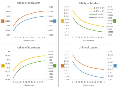
Augmentation of money demand enables to prescribe on the varying inflation rates considering the welfare costs of inflation tax. Social planner can set a implausibly high inflation rate, without accounting for money holding decisions, because doing so would hurt only one type of household, namely the lender, by redistributing away from them. The cashless economy suggests that the borrowers always benefit while the lenders always suffer from higher inflation. In contrast, money-in-utility model demonstrates that the additional distortion in the form of inflation tax can affect even the constrained households negatively, resulting in a welfare loss from generating inflation.

The optimal monetary policy in the sense of a specific inflation rate offer is beyond the scope of Chapter 2. Instead, it is concerned with the long-run role of the monetary policy, how it influences patient and impatient households; and hence, affects utilitarian welfare. In turn, it attempts to provide a prescription to a policy planner in setting inflation rate. In this regard, this chapter shows that the inflation rate has long-run real impacts, disproportionately affects heterogeneous households by redistributing from lenders to borrowers with anticipated inflation; and whether the inflation rate can be used as an instrument to improve utilitarian welfare relies on the presence of money de- mand in the form of money-in-utility model, the concern with pro-lender/borrower bias, the relationship between intertemporal elasticity of substitutions and the heterogeneous productivity levels. In other words, the policy planner should be concerned about these features when targeting an inflation rate to account for the welfare effects of that policy implication.

1Campbell and Viceira (2001).

Chapter 1: Introduction 4 This chapter can also be considered as a guide for monetary policy makers in a glob- ally interlinked environment. With an analogy of developing countries as borrowers and developed countries as lenders, this chapter suggests that an equilibrium inflation initi- ated for the benefit of the lenders is likely to be harmful for the borrowers and in turn social welfare worsening. The same proposition can also be applied to the economic and monetary unions as they are bound by the decisions of the planner institution.

In unions, the member countries, where not all of the economies exhibit the same ad- vancement in terms of characteristics and the structure with each other, are subject to non-customized decisions of the policymaker institution. This study suggests that the actions by the monetary authority can still achieve union-wide welfare gain although the particular policy benefits only some of the participant countries on the cost of a loss for some of the countries embodied in the union, accounting for the above stated factors.

Particular example in this case could be European Union where the member countries are tied by the decisions of the European Central Bank (ECB). Some countries in the union such as Germany and Sweden are having relatively better economic conditions than other countries such as Greece and Bulgaria. Among these member countries, some funds are changing hands in order to sustain the solidarity in Europe. Keeping in mind that the ECB has a target of %0.2 inflation rate, this chapter place a question mark on the discussion whether such a target impairs the recipient countries or donor countries of these funds.

Most central banks share the same aim of achieving price stability although each re- quires to consider the structure and the characteristics of its own economy. With an approach taking into account these differences, sources and responses of inflation can be exhaustively elaborated. In the literature, the empirical strategies for examining the determinants of inflation, in general, can be classified into two. First, the pattern of inflation in a single country over a long horizon can be studied. Over 50 or 100 years, there may be sufficient changes in inflation and institutions so that meaningful tests on different theories of inflation determinants can be checked. Secondly, the experiences in several different countries over a shorter time span can be compared as the differences in economical and political drivers among countries serve for an understanding of the inflation dynamics. Following the second strategy, in Chapter 3, the determinants of inflation in emerging market and developing countries are investigated.

Understanding the factors driving inflation changes is vital for several reasons. Inflation

affects economic agents unequally by redistributing from one group to another. In other

words, it shifts the purchasing power of some group to another. Investment decisions

are discouraged by inflation as it engenders uncertainty about future. The attempts of

central banks’ trying to control the inflation rate may provoke revaluation of currencies

hindering foreign demand. Alternatively, in the absence of any reactions by the central

banks, inflation tends to cause currency devaluation, giving rise to a vicious cycle that leads to hyperinflation. When the sources that cause fluctuations in inflation expec- tations are known, the conduct of monetary policy is eased as it improves the ability of the central bank to evaluate its own credibility and to assess the influence of its policy actions. To avoid the negative effects of inflation on economy and be able to pin- point optimal reactions, diagnosing the determinants of inflation and the transmission of shocks together with interrelationships between inflation and economic factors are crucial, adding to the understanding of the inflation dynamics.

Chapter 3, first, presents an extensive review of the literature on the determinants of inflation. Then, it aims to improve the knowledge on inflation dynamics with two types of annual data by incorporating different theories on the drivers of inflation. The proximate determinants refer to exchange rate, unemployment rate, money growth, oil price and public debt. Next, the analysis continues with a focus on institutional factor, socio-economical and political characteristics of the countries. In particular, central bank independence index, income inequality and political structure index are considered as sources of inflation. The findings demonstrate that inflation is mainly driven by money growth and inflation persistence when only proximate variables are considered.

From the political perspective, greater democratization is found to lead to inflation as the inequality gap rises. The insignificance of the impact from de juro central bank independence on inflation is supported. In each specification regardless of the focus for the determinants of interest, the positive effect of the inflation inertia is shown to be the greatest in terms of both magnitude and significance, suggesting that the inflationary expectations and indexations schemes in price and wage are the most critical determinants of inflation in emerging and developing economies.

The results of this positive analysis give rise to the following policy implications. If the dominance of inflation inertia is claimed to be backward-looking wage settlements, wage negotiations should be arranged on productivity instead of past realizations of inflation in the future. Since the first round effects of adverse supply shocks could be amplified in a volatile environment affecting inflation expectations and credibility of the monetary authorities in applying policy regime, structural reforms should be considered. If the inertia is proven to arise from inflationary expectations with slow adjustment, price controls, such as controlled levels of exchange rate, wage and prices, may accelerate the adjustment of the expectations breaking the inflation inertia.

Inflationary inertia can also be broken when the monetary authority would be forward-looking and more responsive to the deviations of expected inflation from the inflation target. It tends to be reduced with credible disinflationary policies and plans. To maintain the downward

2It is important to note that these choices may lead to unemployment, shortages and speculative effect on exchange rate.

Chapter 1: Introduction 6 pressure on prices considering that inflation persistence is due to staggering of price- setting and price-indexation especially accompanied by high public sector deficit, control over the price of consumer goods and public services; and cuts in subsidies can be used.

The novelty of the analysis in Chapter 4 arises from the question that regarding the best response of the monetary policy authority is in aid recipient developing countries. The Millennium Development Goals emerged from the September 2000 Millennium Decla- ration at the United Nations and include measurable targets for halving world poverty between 1990 and 2015. Especially with these targeted goals, numerous studies on for- eign aid have been entailed. Considering the fact that foreign aid in some less developed countries is quite substantial, it is evident that monetary authorities should not neglect these inflows in setting their monetary policies as the policy regime they follow has an impact not only on prices but also on the allocation of resources.

The development economists argue that an effective redistribution of resources from industrialized countries to developing countries is necessary in order for the poor coun- tries to catch the rich ones. In doing so, foreign aid is suggested to fill up the gap between these country groups. The underlying assumptions for this growth stimulus idea are that the additional resources will be used for investments; and the most of the additional income that is generated from these productive investments will be saved and used for other productive projects. Hence, many donor countries tie their aids to specific projects in order to ensure the efficiency of the aid. Alternatively, growth stimulating effects of foreign aid are conditioned on the environmental, institutional and policy fac- tors. As it can be observed from the literature, while most of the early contributions are predominantly empirical and concentrate on the growth effect of foreign aid, the limited number of theoretical papers that combines monetary policy and foreign aid concen- trates either on the role of monetary policy in limiting the negative impacts of foreign aid or in a positive analysis. However, Chapter 4 aims to fulfill the normative analysis gap on this topic by comparing the optimal monetary policy responses in aid-receiving countries.

In this vein, in a New Keynesian model augmented with foreign aid, policy parameters of the Taylor rule, namely interest rate smoothing, inflation targeting and output growth targeting, are optimized in order to maximize unconditional welfare under three cases:

(i) only cost-push shock (CP ), (ii) only foreign aid shock (F A); and (iii) cost-push

and foreign aid shocks (CP + F A). Initially, a theoretical model where the government

receives the foreign aid and directs it to the representative household as a lump-sum

monetary transfer is constructed. Next, foreign aid is designed to be entirely spent on

consumption goods that the household has no control over the decision on; yet, still

derives utility from.

The results demonstrate that aid recipient developing countries also face a trade-off

between stabilizing the inflation rate and output growth in the presence of cost push

shock. The reason behind this finding is that cost push shocks directly affect prices

whereas foreign aid has no direct impact on prices, yet influences the allocations through

which affecting prices. Hence, the trade-off between two monetary targets does not

vanish, making the inflation targeting still more desirable compared to output targeting

in these countries. The findings also indicate that central banks exhibit non-desirability

of responding to the output growth in the presence of foreign aid shock. The qualitative

effects of a foreign aid shock are very similar to those of a positive productivity shock and

preference shock in wealth transfer and consumption transfer setting respectively. By

increasing output in the former; and consumption in the latter settings, foreign aid shock

reduces the distortion introduced by cost-push shock; hence, facilitating the stabilization

of the output growth. In other words, as an extra income or consumption, foreign aid

supports the monetary policymakers by eliminating the trade-off that they are facing by

mitigating the effects of the nominal rigidity that exists in the economy. In short, foreign

aid is found to resolve the trade off between inflation and output stabilization faced by

the monetary authority, leading to the conclusion that foreign aid recipient developing

countries should act in favor of the inflation targeting as in industrialized countries.

Chapter 2

Disentangling the Impacts of Anticipated Inflation

2.1 Introduction

Most of the central banks aim inflation targeting where the positive rate of inflation target has a range between 1 percent and 3 percent (Bernanke and Mishkin (1997)).

However, the welfare effects of such a policy implication are still debatable. Since many assets and liabilities are fixed in nominal terms, rather than being inflation-indexed, unanticipated inflation lowers the real value of nominal assets and liabilities, thereby redistributes wealth from lenders to borrowers. Hence, any elaborate analysis on re- distribution of inflation necessitates abstaining from representative-agent models and focusing on heterogeneous agent models. Although superneutrality of money implies that the real economy is independent of the rate of money supply growth in the long run; and inflation has no real effects in the long run with lump-sum taxes, dynastic households and complete capital markets (Lucas (2000)), there are empirical studies that suggests otherwise, such as Bullard and Keating (1995)

and Kahn et al. (2006)

to name a few; and non-neutrality of inflation has also been theoretically demonstrated to be present when inflation has redistribution across generations (Weil (1991)) and when inflation has an impact on distortionary taxes (Chari et al. (1996)).

This chapter proposes a theoretical model with two types of households to explore the distributional effects of inflation and assess the non-neutrality of money without aggre- gate and idiosyncratic risks, distortionary taxes or generational gap. The differences

1They show that changes in money growth rate affect output level.

2They find that a small rise in money growth rate in economies which have a low inflation rate increases the long-run capital stock level.

8

in time preference of households define their types as lenders or borrowers. When in- troduced, different labor productivity levels create income inequality among the types per se. Both type of households optimize intertemporally while impatient borrowers are subject to the borrowing constraint; and the equilibrium level of lending and borrowing is endogenized. Although there is no risk in this setting, bond market can be considered as incomplete with nominally non-contingent bonds. Bonds are non-contingent in the sense that when the period of maturity comes for repayment, the amount of repayment is diminished by the inflation rate at the time of maturity and the time preference of the borrowers due to the period difference between obtaining the loan and maturity.

Moreover, a less developed financial market where neither future income nor durable goods can be pledged for securitization of the debt obligation is considered such that lending is restricted by current income.

This, however, results in a nominal friction, as higher inflation reduces the real value of debt in terms of commodities at maturity, which tends to benefit borrowers. Therefore, even anticipated inflation becomes non-neutral where the borrowing constraint causes non-neutral effects in employing monetary policy.

Additionally, since the debt contracts are predetermined in nominal terms, inflation can influence the net worth of borrowers. In particular, an increase in inflation rate lowers the real debt repayments for given outstanding debt; thereby redistributing from lenders to borrowers.

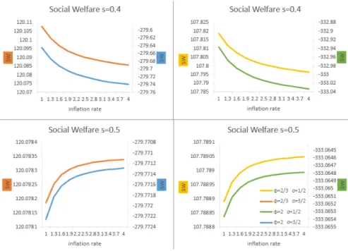
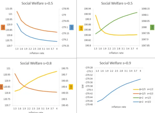
In order to depict the non-neutrality of inflation and to gauge the redistributional ef- fects, simulation exercises are conducted. They demonstrate that there is a conflict of interest on inflation between the borrowers and the lenders as the welfare of borrowers rises with inflation whereas that of lenders decays in all parameterizations, revealing the redistributional effect of inflation. Due to the welfare gain that the borrowers could attain by having high inflation, they would always prefer higher inflation rates than the lenders. Hence, this would cause a corner solution at either of the extremes in determina- tion of inflation rate unless there is a social planner. A simple calculation of utilitarian welfare with different weights attached to two types shows that the importance that is given to the borrower in the utilitarian welfare by the hypothetical social planner matters. Specifically, utilitarian welfare can be decreasing in inflation with low weights (i.e s < 0.5) attached to the borrower depending on the parameterizations, thereby re- vealing that the negative impact of inflation on lenders outweighs the positive impact on borrowers when the social planner has pro-lender bias. In principle, a benevolent social planner who aims to maximize utilitarian welfare would act in favor of the con- strained household. In this vein, since the borrowing constraint is the only distortion

3The termincompletefinancial market is used here in a slightly different terminological way than the literature has been using. For instance, as in the explanation of Sheedy (2016), the financial markets are called incomplete when the debt contracts cannot guarantee the debt repayments for all future event realizations.

4See, such as Laibson, Repetto and Tobacman (2003), Korinek (2009) and Bianchi (2011).

Chapter 2: Disentangling the Impacts of Anticipated Inflation 10 in the economy, the social planner would set the inflation rate such that this friction is minimized. However, the utilitarian welfare highlights that even without favoring the borrowers, increasing welfare is achieved. Since this result is attained regardless of the assumption on the productivity levels, it can be said that the monetary policy redistributes resources from lenders to borrowers by generating inflation. Further, the comparison of changes in the productivity levels reflects that when the heterogeneous productivity levels are assumed, the utilitarian welfare gain is larger in both magnitude and level than the gain in the equal productivity case. Specifically, the welfare gain is larger in between 12.5-31% in heterogeneous productivity case than its homogeneous counterpart. As a result, the heterogeneous productivity levels form the second channel for redistribution. Hence, this chapter can be accounted for a further support to the existing empirical and theoretical literature for the positive relationship between income inequality and inflation. In particular, Crowe (2006), Dolmas et al. (2000) and Desai, Olofsgard and Yousef (2005) among many others, identified a positive relationship be- tween these variables with different theoretical settings and empirical analyses. In this study, different labor productivity levels also facilitate the income inequality among the types and the simulation exercises quantify that the welfare gain from generating infla- tion is higher when income inequality (i.e heterogeneous labor productivities) is present, thereby suggesting that the policy planner can achieve more welfare gain by generating higher inflation when there is income inequality.

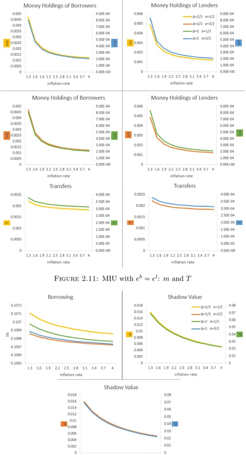
The money demand motive is introduced to the economy in order to assess the welfare effects of inflation in a setting where decisions regarding to money holding generate another distortion in addition to the borrowing constraint. Augmentation of money demand enables to prescribe on the varying inflation rates considering the welfare costs of inflation tax. Money in the utility (MIU) models, in principle, necessitates zero nominal interest rate in order to cancel out the opportunity cost of holding money when it is the only source of distortion; and by the Fisher relationship, it follows that the optimal changes in prices requires deflation (i.e Friedman Rule). Hence, in order to consider these corresponding relationships, investigating the effects of monetary policy requires a model with cash as the money demand is affected by the changes in inflation.

Without accounting for money holding decisions, social planner can set a implausibly

high inflation rate, because doing so would hurt only one type of household, namely the

lender, by redistributing away from them. However, the introduction of money demand

incurs the same distortion that is generated in the form of inflation tax on both types,

preventing the social planner from choosing such a high inflation rate. Hence, the aim

in this analysis is to distinguish the effects of inflation under the presence of money

demand motive and compare the welfare consequences of inflation tax in this economy

with the cashless economy so as to provide a guideline to the policy planner in setting

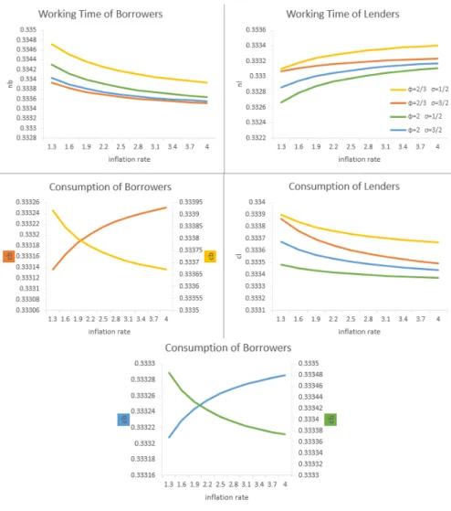
inflation rate. The results from the simulations imply that the additional distortion in the form of inflation tax can affect even the constrained households negatively, resulting in a loss in the utilitarian welfare from generating inflation. When borrowers are worse off because of the higher inflation, this renders a welfare loss as the lenders are always hurt by higher inflation. Nevertheless, the cases where the borrowers are better off due to higher inflation do not translate into welfare gain when the types are equally treated in the utilitarian welfare function, suggesting that the loss of the lenders are larger than the gain of borrowers from higher inflation. Furthermore, when the households take multiple decisions in addition to money holding, the relative magnitudes of intertemporal elasticity of substitutions (IES) of these choices have to be taken into account when setting inflation rate. In particular, when both inverse IES of labor and consumption are higher/lower than that of real money balances, the combination of effects from labor and consumption decisions is mirrored on the utility of borrowers. On the other hand, when only one of the inverse IESs is higher than that of the real money balances together with the smaller one being the inverse IES of consumption, the effect of real money balances designates the outcome on the utility of the borrowers. These results follow from the fact that the elasticity of marginal utility with respect to consumption has the largest impact on the utility of borrowers even when it is lower than real money balances and labor supply as there is no scale parameter that restricts its effect on the utility.

From the theoretical perspective, redistributional effects of monetary policy in the liter-

ature are generally attributed to unanticipated inflation changes and exogenous hetero-

geneity between households. In their paper, Beetsma and Van Der Ploeg (1996) define

the inequality in a society where larger part of the government debt is held by the smaller

group of individuals and heterogeneity arises when agents have different productivity of

labour, thereby building up different stocks of assets. When the wealth is unfairly dis-

tributed, the median voter is more likely to be the poor. Hence, it is in the interest

of the government to favor the poor; and in return, they levy unanticipated inflation

taxes to erode the real value of debt, in an attempt to redistribute from rich to poor

as this would hurt the rich more than the poor. Albanesi (2006) designs a bargaining

game for the determination of the inflation between heterogeneous agents where they

differ in their labor productivities and access to various payment methods, in which low

income households hold more cash and hence, are more vulnerable to inflation. A large

gap in labor productivities translates into larger inequality which generates a weaken-

ing in the bargaining position of the poor and, in turn, causes higher inflation as it is

desired by the rich. Hence, the redistributional effect of inflation relies on the equilib-

rium differences in transaction patterns across households which depends on the labor

productivity differences. Pescatori (2007) investigates optimal monetary policy in an

Chapter 2: Disentangling the Impacts of Anticipated Inflation 12 environment where rich and poor households are categorized according to an exogenous distribution of assets; and the inflation is found to have redistributional effects on rich and poor. The redistributional consequences of inflation in this chapter, however, are based neither on different productivity levels nor unexpected inflation changes. Inflation has a direct impact on household’s net worth by reducing the maximum amount of debt that can be issued as the debt contracts are agreed in nominal terms. Due to the lowered real value of debt repayment received by the lender from the borrower, even expected inflation has redistributive effects from lenders to borrowers. In order to disentangle the effects of heterogeneous productivity levels, different productivity levels are introduced in the simulation exercise. Although the amplification of the redistributional effects from monetary policy is observed, redistribution is found to be still present even with homogeneous productivities.

Non-neutrality of monetary policy is in general investigated in theoretical frameworks where models have aggregate or idiosyncratic risks, capital market imperfections, capital tax distortions, labor supply distortions or distortionary redistribution of seigniorage.

Algan and Ragot (2010) analyze the long-run effect of monetary policy where hetero- geneous households face credit constraint and can partially insure themselves against idiosyncratic income shocks by using capital holdings and real balances. They show that the inflation has real effects as long as the financial borrowing constraint is bind- ing as it would induce endogenous decision making in money demand. Sheedy (2016) studies the monetary policy targeting in an incomplete financial market setting where aggregate uncertainty in output results in non-contingent debt contracts as not all the future events are guaranteed for repayment. He shows that in the case where there is no uncertainty about the growth of real output and no unexpected changes in inflation, the equilibrium steady state is independent of monetary policy. Doepke and Schneider (2005) provide a calibrated OLG model to assess the inflation-induced redistribution under different fiscal policy rules. In their paper, there is no idiosyncratic labor income risk, yet, the heterogeneity in earnings is generated by the differences in skill profiles;

and they are concerned with unanticipated inflation shocks on nominal asset holdings as

these shocks would urge different positioning in portfolios of the households. They find

that the redistribution caused by inflation has a negative effect on output. In this regard,

the real effect of inflation rests on the choice of model setting. Specifically, OLG model

gives rise to life-cycle effects in which the borrowers are the winners and the lenders are

the losers. Since the borrowers tend to be younger than the lenders, the net effect is ob-

served in aggregates. However, the theoretical model in this chapter is populated by two

types of households, namely patient and impatient, generated by heterogeneity in time

preferences and it is the same assumption that assures the binding borrowing constraint,

which is the essence of this analysis as the otherwise would imply representative-agent

model. Therefore, the contribution of this chapter to the literature is that even in the absence of idiosyncratic income shock, of market incompleteness stemming from aggre- gate risk, of utilization of OLG model and of money demand together with anticipated inflation, changes in inflation has real effects.

There are only few papers which study the impact of anticipated inflation in hetero- geneous agent economies. The existing heterogeneous-agent monetary economy studies examine the settings where money is valued, at least partly, as it grants the agents with self-insurance against idiosyncratic shocks (such as Molico (2006), Chiu and Molico (2010)). The motivation for holding money in these papers is derived from market tim- ing frictions, cash-in-advance constraints, precautionary role of money and so on. They differ in whether the money is the only available asset for agents’ portfolio decisions and also in their results. Akyol (2004) considers a pure exchange, incomplete market economy in which agents hold bonds and money for precautionary purposes against id- iosyncratic productivity shocks. A market-timing friction ensures that in equilibrium only the high-endowment agents hold money as it allows for consumption smoothing.

While bonds and money pay the same return at zero nominal interest rate, bonds allow for borrowing. Hence, positive inflation induces the bond demand while reducing the money demand of high-income agents by improving risk sharing. In turn, this effect redistributes income from the high- to low-income agents. The key finding of the paper is that 10% inflation is necessary in order to maximize social welfare. Molico (2006) introduces a random matching model where agents are hit by i.i.d shocks that restrict them to be a buyer or a seller and suggests that if inflation is low, higher inflation can enhance social welfare as it decreases price dispersion and wealth.

On the contrary, Wen (2010) reports that 10% inflation costs at least 8% of per-capita

consumption. This paper is built up on a production economy where agents hold capital

and precautionary money and inflation eliminates the self-insurance of money. In their

matching model, Boel and Camera (2009) address that inflation does not cause large

losses in social welfare; yet, the consequences on distribution can be immense, depending

on the financial structure of the economy. Specifically, mostly the wealthier is hurt by

inflation if the money is the only asset; and if assets other than money are available,

inflation can harm the poorer households while benefiting the wealthier. Camera and

Chien (2014) examine an economy where ex-post heterogeneity is formed with labour

productivity shocks that follow a Markow process, agents are allowed to hold money

and bond considering cash-in-advance constraint and the money supply evolves deter-

ministically. They show that the inflation non-linearly affects the distribution of income

with the strongest impact when small deviations from zero inflation occur; and suggest

that the financial structure, the labor supply elasticity and the shock persistence al-

ter how distributions and welfare are influenced by inflation. In particular, when only

Chapter 2: Disentangling the Impacts of Anticipated Inflation 14 money is available in self-insurance, inflation alleviates wealth disparities; otherwise, it may rise wealth inequality. In contrast, this chapter does not incorporate money into the framework to ensure self-insurance in the form of precautionary money demand. In other words, rather than substituting as a tool for guarantee, attaching value to money introduces an additional friction to the economy in the form of inflation tax. Addition- ally, this study endogenizes the labor supply decision and money creation

which some papers (e.g. Akyol (2004) and Camera and Chien (2014) respectively) in the literature lack; and attempts to reconcile the divergent results in this line of literature.

The remainder of the chapter is as follows. Section 2.2 lays out the model environment.

Section 2.2.1 defines the equilibrium of the cashless economy, Section 2.2.2 discusses the steady state of the cashless economy and Section 2.2.3 contains the simulation exercises of the cashless economy. In Section 2.3, MIU model is introduced and the equilibrium together with simulation results of this environment are presented. Finally, Section 2.4 concludes.

2.2 Theoretical Model: Cashless Economy

The discrete time, infinite horizon model is populated by two types of households, patient and impatient. The heterogeneity in households stems from the difference between their time preference in addition to labor productivity. Both types of households decide on how much to consume, work and hold assets in the form of bonds. Additionally, impatient households are allowed to accumulate debt funded by patient households.

Competitive firms produce the final good by utilizing the labor supplies from both types of households. Monetary policy is assumed to control the inflation rate.

The patient households differ from the impatient ones as they exhibit higher patience rate. This, in return, defines their position towards bond holding, which identify them as lenders or borrowers. The interaction between the borrowers and the lenders, therefore, occurs in the bond market. Lenders hold the bonds issued by borrowers in the sense that what is defined as inflow for one type means outflow for the other type of household.

There is no explicit default and aggregate uncertainty in the economy. Yet, bond market can be considered as incomplete with nominally non-contingent bonds. Bonds are non- contingent in the sense that when the period of maturity comes for repayment, the amount of repayment is diminished by the inflation rate at the time of maturity and the time preference of the borrowers due to the period difference between obtaining the loan and maturity. In addition to this, a less developed financial market where neither

5How the real money balances grow root in the decisions of the two types of households instead of exogenously given rate. See equations (2.34), (2.35) and (2.22), (2.27).

future income nor durable goods can be pledged for securitization of the debt obligation is considered such that lending is restricted by current income. Monetary policy has direct impact on household’s net worth by diminishing the real value of outstanding debt by determining a path for the price level.

The borrowers maximize a lifetime utility function given by max

{c^b_t,b^b_t,n^b_t}

∞

X

t=0

β

(c

)

1 − φ − ν (n

)

1 + σ

!

where the discount rate is β ∈ (0, 1), φ and σ denote the inverse elasticity of substitution for consumption and labor supply respectively; ν weighs the disutility from working, c

is the consumption, n

are working time.

The budget constraint is

P

c

+ B

≤ e

P

w

n

+ B

R

where B

represents the nominal debt, R

denotes the nominal interest rate on debt; so that,

t

is the current nominal value of debt issued (i.e discount bond) while B

is the debt repayment. The left-hand side of the budget constraint indicates the uses of funds (i.e. consumption spending plus nominal debt service) while the right-hand side denotes the available resources (i.e new debt plus nominal labor income).

In addition to the budget constraint, the borrowers face a borrowing constraint in which the maximum amount B

is bounded by:

B

≤ γe

P

w

n

where γ ∈ (0, 1) represents propensity to raise debt, e

denotes the productivity level and w

is the real wage. In general, γ can be broadly thought of as an indirect measure of the tightness of the borrowing constraint. Notice that the decision towards labor supply endogenously affects the borrowing limit and the debt obligation is bound by the current income.

Household debt, in general, can be categorized into two groups, namely non-collateralized

debt and collateralized debt. At the theoretical level, alternatives to this type of credit

constraints are given in terms of durable goods, such as land and housing, in the case of

collateralized debt (Kiyotaki and Moore (1997), Iacoviello (2005) among many others),

of exogenous net indebtedness limit (such as Zeldes (1989)) and of tradable goods in an

open economy context (see, Monacelli (2006)). However, this is a closed economy model

and there is no durable goods market in order to be attached to the loan as collateral.

Chapter 2: Disentangling the Impacts of Anticipated Inflation 16 In his paper, Korinek (2009) models the borrowing on the current income in which the borrowers are able to engage in fraud at the contract period and if the lenders disclose the fraud, they could seize the current income of the borrowers. Although this type of contract enforcement scheme is not explicitly addressed here, it is accounted for that the debt repayment cannot always be guaranteed due to the lack of securitization of the debt obligation. Bianchi (2011) also designs the credit constraint such that loans amount to a debt that is a fraction of tradable and nontradable current income. Such modelling can be attributed to less developed financial markets where sophisticated fi- nancial instruments, compared to income, such as collateralized debt obligations are not available. Hence, the lenders can only guarantee the repayment of the borrowers, similar to Laibson, Repetto and Tobacman (2003)

, by evaluating the borrowers accord- ing to their current income. In turn, loans provided by the lenders are assumed to be conditioned on the current income of the borrowers. In his paper, Fafchamps (2014) also emphasizes that granting the poor in developing countries with credit depends on whether they have regular income rather than collateral.

At the empirical level, there are studies supporting the assumption that the borrowing constraint is given by the current income. For instance, Japelli (1990) shows that the current income is a major determinant of the credit market access. Del-Rio and Young (2005) examine the determinants of participation in the unsecured loan market for 1995 and 2000 in the U.K and find that the main determinant is the individual income level.

Additionally, Mishkin (1996) notifies that the legal system in developing countries makes securing the credits with collateral a time-consuming and costly process. Hence, attach- ing income for securitization of the debt obligation can be referred to both developing and developed country contexts.

The lender households maximize the following utility function subject to a budget con- straint

max

{c^l_t,b^l_t,n^l_t}

∞

X

t=0

δ

(c

)

1 − φ − ν (n

)

1 + σ

!

subject to P

c

+ B

R

≤ e

P

w

n

+ B

where δ > β and e

> e

.

The constraints of the households can be rewritten in real terms. For the borrowers, the budget and the borrowing constraints follow c

+

bt−1

πt

≤ e

w

n

+

t

and b

≤ γe

w

n

respectively where π

=

t−1

is the gross inflation rate. The important feature of the budget constraint roots in the debt contracts’ being predetermined in nominal terms;

6In their paper, they have two types of debt, collateralized and non-collateralized. To model non- collateralized borrowing, they introduce a loan limit which is proportional to current income.

so that, the inflation rate can influence the net worth of the borrowers. In other words, an increase in inflation rate lowers the real debt repayments for given outstanding debt.

For the lenders, the budget constraint reads c

+

t

≤ e

w

n

+

l t−1

πt

. It is important to differentiate between the available debt services to the borrowers and the amount of debt obligations for repayment. The maximum amount of real (nominal) debt that the lenders provide the borrowers is b

(B

). They limit this amount, in order to secure the debt services they can offer to the borrowers, to the income of borrowers, rather than the debt repayment. In this vein, when they lend, the lenders hold the discount bonds issued by borrowers with a face value of

t

, and in return, receive back the amount of

b^l_t−1

πt

from the borrowers when the period of maturity comes. Therefore, the value of borrowing limit, B

, is not affected by the inflation rate while the real debt repayment (i.e real value of outstanding debt),

lt−1

πt

, decreases with the inflation rate.

The first-order conditions for the borrowers require the marginal rate of substitution between labor supply and consumption and Euler Equation for labor supply respectively:

ν(n

)

e

w

= (c

)

+ γϕ

ν(n

)

e

w

− γϕ

! 1 R

= βE

ν(n

)

e

w

− γϕ

! 1 π

! + ϕ

where ϕ is the Lagrange multiplier associated with the borrowing constraint that takes positive values whenever the constraint is binding. Specifically, the borrowing constraint is binding at the steady state due to the assumption on time preferences.

Notice that, in the absence of borrowing constraint (i.e., ϕ

= 0), the terms with ϕ

drop out. In- tuitively, if ϕ

increases, the borrowing constraint binds more tightly; in other words, the marginal gain from relaxing the constraint is larger. Therefore, the marginal gain from supplying an additional unit of labor is higher as it allows to increase borrowing.

Furthermore, as it can be seen from the first equation, the higher the marginal value of an additional borrowing, (i.e ϕ

), the higher the benefit of providing an additional unit of working time (i.e

> (c

)

), which will be used to purchase an additional current consumption. Due to the binding borrowing constraint (i.e ϕ

> 0), the bor- rower’s marginal utility of current consumption exceeds the marginal utility of savings (i.e

t

> β E

(c^b_t+1)^−φ

πt+1

). Consequently, they would like to increase the consumption spending more than the lender who acts as a consumption-smoother. In order to obtain that amount, the borrower has to optimally choose how much to borrow as it will depend on the increase in working time considering that would also cause disutility to them.

7See equation (2.13) for proof.

Chapter 2: Disentangling the Impacts of Anticipated Inflation 18 The solution to the lender’s problem requires:

ν(n

)

e

w

= (c

)

(n

)

w

1 R

= δ E

(n

)

w

1 π

!

the substitution between consumption and labor choices and Euler Equation for labor supply respectively.

The comparison between the first-order conditions of both types of household yields the differences in their decision making due to the borrowing constraint faced only by the borrower. In particular, in the absence of the borrowing constraint (i.e. ϕ = 0), ϕ drops out both sides of the labor Euler equation of the borrowers and the equation reduces to a standard intertemporal condition which would prevail for the lenders except the discount factor.

Competitive firms produce the final goods according to the following linear production function utilizing total labor supply n

:

y

= e

n

and z

is the technology that follows an AR(1) process z

= ρz

+ e

where e

is the independent, serially uncorrelated innovation and normally distributed with zero-mean and standard deviation σ

.

This is a cashless economy where money is not needed for any transactions. Since there is no cash, the monetary authority is only responsible for determining the inflation rate, π

.

2.2.1 Competitive Equilibrium

A competitive equilibrium is a set of sequences {c

, c

, n

, n

, b

, b

, y

, n

, w

, R

, ϕ

, z

}

satisfying

For households:

ν(n

)

e

w

= (c

)

+ γϕ

(2.1)

ν(n

)

e

w

− γϕ

! 1

R

= β E

ν(n

)

e

w

− γϕ

! 1 π

!

+ ϕ

(2.2)

b

= γe

w

n

(2.3)

c

+ b

π

= e

w

n

+ b

R

(2.4)

ν(n

)

e

w

= (c

)

(2.5)

(n

)

w

1 R

= δ E

(n

)

w

1 π

!

(2.6) (2.1), (2.2) and (2.5), (2.6) are the first-order conditions for the borrowers and the lenders respectively.

(2.3) and (2.4) are the constraints for the borrowers.

Market clearing conditions:

c

+ c

= y

(2.7)

e

n

+ e

n

= n

(2.8)

b

+ b

= 0 (2.9)

(2.7) for goods market, (2.8) for labor market and (2.9) for bond market.

The production follows:

y

= e

n

(2.10)

z

= ρz

+ e

(2.11)

w

= y

n

(2.12) where (2.12) is the solution to the firm’s maximization problem.

8Alternative to equations (2.2) and (2.6), would be respectively:

(ctb

)^−φ Rt

=βEt(c^b_t+1)^−φ 1 πt+1

! +ϕt

(ctl

)^−φ Rt

=δE^t(c^l_t+1)^−φ 1 πt+1

!

Chapter 2: Disentangling the Impacts of Anticipated Inflation 20 2.2.2 Steady State of the Competitive Equilibrium

This section analyses the features of the steady state of the competitive equilibrium.

In the deterministic steady state, the constraints are always binding. Starting with the first order condition with respect to consumption for the borrowers would reveal that the budget constraint has to bind:

c = λ

where λ denotes the Lagrange multiplier of the budget constraint. The similar calcula- tion also holds for the lenders. The borrowing constraint is binding

ϕ = λ δ − β π

!

(2.13) due to the the assumption that the lenders are more patient than the borrowers. There- fore, the shadow value of borrowing is always positive. In other words, the borrower will always choose to hold a positive amount of debt.

The steady state consumption Euler equation of the lenders, (2.6), implies:

R = π δ

Due to the zero lower bound on nominal interest rate, the following restriction entails π ≥ δ.

Combining the result of R with the labor Euler equation of the borrowers (2.2) yields:

ϕ = ν(n

)

e

w

δ − β π + γ(δ − β)

!

> 0 (2.14)

Notice that, β = δ (i.e. no heterogeneity in discount rates) implies that the borrowing

constraint does not bind. Furthermore, this hypothetical assumption would correspond

to a representative agent economy. In order to facilitate the understanding of how

the borrowing constraint alters the equilibrium, consider a model without a borrowing

constraint, yet, with heterogeneous patience rates. No borrowing constraint implies

that the impatient household trades her future working time with current consumption

by borrowing against her future income, causing her consumption to approach to zero

asymptotically. However, with a borrowing constraint, there is a limit on how much the

impatient households can borrow, which will lead to a stable steady state with positive

consumption for both types.