A Sample of Galactic PDRs: [CII] Optical Depth Effects and Self-Absorption

(1)

A Sample of Galactic PDRs: [CII]

Optical Depth Effects and Self-Absorption

Inaugural-Dissertation zur

Erlangung des Doktorgrades

der Mathematisch-Naturwissenschaftlichen Fakultät der Universität zu Köln

vorgelegt von Cristian Guevara N.

aus Copiapó, Chile

Köln, 2019

(2)

Prof. Dr. Simon Trebst

Tag der mündlichen Prüfung: 23.08.2019

(3)

To my Wife, Parents and Grandmother

(4)

(5)

Abstract

The main objective of this work was to determine the optical depth of the ionized carbon and to study the effects that could be arise from this optical depth. For this reason, high spectral resolution and sensitivity observations were done of the [

¹²

CII]

2

P

3/2

-

²

P

1/2

158 µm fine structure line and the [

¹³

CII] hyperfine structure line split- ted into three components. The observations were done simultaneously with up- GREAT 7x2 array receiver on board the airborne observatory SOFIA towards four photodissociation regions covering a wide range of physical conditions: the HII re- gion M43, the edge-on and faint Horsehead photodissociation region, the spherical and highly ionized Monoceros R2 and the massive and clumpy M17 SW. Addition- ally, the M17 complex was observed in [CI]

³

P

1

-

³

P

0

609 µm line in order to study the large scale [CI] emission along M17 SW and M17 N. The observations were done with the SMART array receiver of the NANTEN2 telescope at high spatial and spec- tral resolution.

As a first step, direct comparisons of the [

¹²

CII] and [

¹³

CII] emission line pro-

files and intensities for multiple positions in each source, assuming a single homo-

geneous layer and a reasonable

¹²

C/

¹³

C abundance ratio, have revealed that the

Cp13 line, scaled up by the canonical abundance ratio between

¹²

C and

¹³

C, com-

pletely overshoots the [

¹²

CII ] emission with different line profiles. Thus, [

¹²

CII ] is

optically thick in all sources and, in the case of Mon R2 and M17 SW, is heavily

affected by self-absorption effects. Column densities derived from the [

¹³

CII ] inte-

grated intensity show extremely high column densities, four times higher than the

column densities derived directly from [

¹²

CII ] integrated intensity. This situation

required a more sophisticated analysis. A multi-component dual layer model of

the radiative transfer equation has been developed to take into account the discrep-

ancy between the line profiles of both isotopes,as well as the intensities between

them. The model allows the simultaneous fit of the emission of both isotopes and

the derivation of the physical properties of the [CII] gas, namely column density

and excitation temperature. The model is composed of a background emitting layer

and a foreground absorbing layer. The parameters derived from the model show

extremely high background column densities, up to 10

¹⁹

cm

⁻²

or as an equivalent

visual extinction around 41 magnitudes; and cold foreground column densities up

(6)

ground column densities require multiple PDR surfaces stacked along the line of sight, showing a clumpy structure. The cold high column density foreground gas can not be explained with any known scenario and only speculations can be done to explain its origin.

The M17 SW [CI] observations have shown the velocity distribution of the [CI]

emission and, through the analysis of momenta maps, three distinctive velocity

structures have been identified. Each structure can be associated with HI atomic

gas, H

2

molecular gas and as a part of a foreground molecular cloud associated

to the M17 complex, respectively. The [CI] column density of the complex ranges

between 10

¹⁷

and 10

¹⁸

cm

⁻²

, or in equivalent visual extinction, between 1 and 10

magnitudes. M17 SW has the larger amount of material and the larger column den-

sity. The [CI] spectra are shifted to the redder part of the spectra, with respect to

molecular and ionized tracers. Also, the [CI] equivalent visual extinction is much

lower compared to the other tracers. This can be explained as an expected deficit of

neutral carbon, but precise measurements of the local abundances needed to derive

the extinctions would require the use of numerical models and large scale data sets

of complementary tracers, that will be part of future work.

(7)

Zusammenfassung

Das Hauptziel dieser Arbeit war es, die optische Tiefe des ionisierten Kohlenstoffs zu bestimmen, und Effekte die daraus herrühren. Zu diesem Zweck wurden spek- tral hochaufgelöste Beobachtungen mit hoher Sensititivität von der [

¹²

CII]

²

P

3/2

-

2

P

1/2

158 µm Feinstrukturlinie und den [

¹³

CII] Hyperfeinstrukturlinien, die in drei Komponenten aufgespaltet sind, gemacht. Diese Beobachtungen wurden simultan mit dem upGREAT 7x2 Array-Empfänger an Bord des SOFIA-Flugzeugs in Rich- tung von vier Photodissoziationsregionen (PDR) erlangt, die eine große Vielfalt von physikalischen Bedingungen abbilden: die HII-Region M43, die leuchtschwache

“edge-on” Horsehead Photodissoziationsregion, die sphärische und hochionisierte Monoceros R2, und die massive und klumpige M17 SW Region. Zusätzlich wurde der M17 Komplex in der [CI]

³

P

1

-

³

P

0

609 µm Linie beobachtet um die großräumige [CI] Emission entlang von M17 SW und M17 N zu untersuchen. Diese Beobach- tungen wurden mit dem SMART Array-Empfänger des NANTEN2-Teleskops mit hoher spektraler und räumlicher Auflösung erlangt.

In einem ersten Schritt wurden die Emissionslinienprofile von [

¹²

CII] und [

¹³

CII]

verglichen, sowie die Intensitäten für etliche Positionen in jeder Quelle. Dies geschah

unter der Annahme einer einzelnen, homogenen, emittierenden Schicht und eines

angemessenen

¹²

C/

¹³

C Isotopenverhältnisses. Diese Analyse ergab, dass die mit

dem kanonischen Isotopenverhältnis von

¹²

C/

¹³

C skalierte [

¹³

CII ] Linie komplett

die [

¹²

CII ] Emission mit verschiedenen Linienprofilen übertrifft. Das lässt darauf

schließen, dass [

¹²

CII ] in allen Quellen optisch dick und, im Falle von Mon R2 und

M17 SW, stark von Selbstabsorptionseffekten betroffen ist. Die Säulendichten, die

aus den integrierten [

¹³

CII ] Intensitäten gewonnen wurden, sind extrem hoch; vier

mal höher als die aus den integrierten Intensitäten von [

¹²

CII ]. Diese Situation er-

forderte eine wesentlich anspruchsvollere Analyse. Hierfür wurde ein Zweischicht-

modell mit mehreren Komponenten der Strahlungstransportgleichung erwickelt,

um sowohl den Unterschieden zwischen den Linienprofilen beider Isotope Rech-

nung zu tragen, wie auch den Unterschieden ihrer Intensitäten. Das Modell er-

laubt den gleichzeitigen Fit der Emission beider Isotope und die Herleitung der

physikalischen Eigenschaften des [ CII ] Gases, genauer die Säulendichte und Anre-

gungstemperatur. Das Modell besteht aus einer emittierenden Hintergrundschicht

(8)

lenten visuellen Extinktion von 41 Magnituden; die kalte Vordergrundkomponente hat eine Säulendichte von bis zu 10

¹⁸

cm

⁻²

oder 13 Magnituden. Weiterhin wurde ein Einschichtmodell mit mehreren Komponenten untersucht, doch als physikalisch unwahrscheinlich verworfen. Die extremen Säulendichten im Hintergrund wer- den durch mehrere, entlang der Sichtlinie übereinander liegende PDR Oberflächen erzeugt, die eine klumpige Struktur besitzen. Die hohe Säulendichte des kalten Vordergrundgases kann mit keinem bekannten Szenario erklärt werden und bisher kann zu seinem Ursprung nur spekuliert werden.

Die M17 SW [CI] Beobachtungen zeigen die Geschwindigkeitsverteilung der

[CI]-Emission und es konnten, durch die Analyse der Momentekarten, drei ver-

schiedene Geschwindigkeitsstukturen identifiziert werden. Jede dieser Strukturen

kann mit atomarem Wasserstoffgas (HI), molekularem Wasserstoffgas (H

2

), oder als

Teil der molekularen Vordergrundwolken in Verbindung mit dem M17-Komplex

in Verbindung gesetzt werden. Die [CI] Säulendichte des Komplexes liegt zwis-

chen 10

¹⁷

und 10

¹⁸

cm

⁻²

, entsprechend einer visuellen Extinktion von 1 bis 10 Mag-

nituden. M17 SW hat eine höhere Menge an Material und eine höhere Säulen-

dichte. Die [CI]-Spektren sind relativ zu den molekularen und ionisierten Emissio-

nen zum roten (langwelligen) Teil des Spektrums hin verschoben. Weiterhin ist die

[CI] äquivalente visuelle Extinktion wesentlich niedriger im Vergleich zu den Werter

anderer Indikatoren. Dies kann als ein erwartetes Defizit neutralen Kohlenstoffs

erklärt werden, doch werden hierzu präzise Messungen der lokalen Häufigkeiten

benötigt, um die Extinktion herzuleiten, die wiederum numerische Modelle und

größere Datensätze komplementärer Indikatoren erfordern, was Teil von zukün-

ftiger Arbeit sein wird.

(9)

1 | Introduction

Photodissociation Regions (PDRs) are zones of the interstellar medium (ISM) in which Far-UV photons dominate the thermal balance, chemistry, structure and dis- tribution of the gas and dust of such regions. The incident FUV field photodissoci- ates molecules, photoionizes atoms and molecules and heats the gas and dust. The gas is mainly cooled through fine structure line emission of excited atoms, such as [CII], [OI] and [CI]. These lines are key to study the ISM structure and dynamics.

The [CII] 158 µm fine structure line is one of the brightest emission lines in PDRs and the main cooling line in the atomic and molecular gas. The [ CII ] line is not only used to study the local galactic ISM, but is also used as a star-formation tracer for nearby and high redshift galaxies (eg. Boselli et al. 2002; De Looze et al.

2011; Herrera-Camus et al. 2015) due to its ionization by FUV photons produced by nearby OB stars, creating a link between the star formation activity and the [CII]

emission. Therefore, it is essential to know whether the [CII] line emission is opti- cally thin or thick. The concern to know the optical depth of [CII] has been present since the first observations of [CII]. Russell et al. (1980) refers in the first [CII] ob- servation article that: "Optical depth effects in the 157 µm line may be significant but have not been taken into account in our calculations because our data base is still too re- stricted". Traditionally, [CII] has been considered as an optically thin line with an optical depth around unity, but systematic measurements of the optical depth has been only done in a few cases in the last years.

As this issue has not been sufficiently addressed, the main objective of this work was to determine the optical depth of the ionized carbon, to study the effects that could be arise from this optical depth and determine the physical parameters of the ionized carbon through the observations of [

¹²

CII] and [

¹³

CII]. This key analysis has not been done before because, just recently, it has been tecnically feasible to observe both lines simultaneously at high sensitivity and spectral resolution.

Additionally, a fundamental element in the development of a new generation

of receivers and observatories, is to have a selection of targets that may act as test

(14)

cases for the future observations. Hence, for one of the sources observed in [CII],

observations were done in [CI] to be used as a pathfinder for large scale mapping of

star forming regions. Therefore, an additional objective for this work was to study

the large scale [CI] emission of the observations mentioned above.

(15)

2 | Physical Background

The present chapter explains the physical framework required to understand the emission of radiation by atoms and molecules in the GHz and THz frequency regimes studied for this work. This chapter outlines the basic physics of the radiation pro- cess, describes photodissociation regions in which the line emission originates, as well as details the characteristics of the different atoms and molecules employed in this work. The physical background is based on the following books: Radiative Processes in Astrophysics (Rybicki & Lightman 1979), The Physics and Chemistry of the Interstellar Medium (Tielens 2005), Tools of Radio Astronomy (Wilson et al. 2009) and Physics of the Interstellar and Intergalactic Medium (Draine 2011).

2.1 Radiation

The electromagnetic radiation can be considered as waves or photons of the elec- tromagnetic field which radiate through the space, traveling in straight lines called rays. Hence, the energy of a ray crossing an area dA normal to the direction of the ray within a solid angle dω in a time dt in a frequency range dν can be defined as:

dE = I

_ν

dA dt dΩ dν (2.1)

Where, I

ν

represents the specific intensity in units of erg s

⁻¹

cm

⁻²

ster

⁻¹

Hz

⁻¹

. By definition, the specific intensity I

_ν

is constant, as long as there is no emission or absorption. In particular, it is constant along the ray, independent of the distance to the source. Additionally, and knowing that the radiation propagates at the velocity of light c, the specific energy density u

ν

is defined as the amount of energy contained in a volume of length cdt and area dA :

dE = u

_ν

(Ω) dA c dt dΩ dν (2.2)

(16)

Combining both equations above, u

_ν

(Ω) results in:

u

_ν

(Ω) = 1

c I

_ν

(2.3)

Therefore, the mean intensity J

ν

can be defined as:

J

_ν

= 1 4π

Z

I

_ν

dΩ (2.4)

2.2 Planck Function

2.2.1 Planck Spectrum

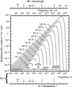
The Planck spectrum describes the electromagnetic radiation emitted by a black body i.e. a radiation source in thermal equilibrium. A proper derivation can be found in physics textbooks such as Radiative Processes in Astrophysics (Rybicki &

Lightman 1979). Thus, the specific intensity defined above in case of thermal equi- librium is described by the black body emission B

_ν

(T ) , for a given temperature T and frequency ν, as:

B

_ν

(T ) = I

_ν

(T ) = 2hν

³

c

²

1 e

^hν/k^B^T

− 1 (2.5)

with k

B

the Boltzmann’s constant (1.38 × 10

⁻¹⁶

erg K

⁻¹

). Figure 2.1 shows B

ν

(T) at different temperatures, on a double logarithmic scale.

2.2.2 Radiation and Rayleigh-Jeans Brightness Temperature

At low frequencies and at sufficiently large temperatures (>20 K), hν << k

_B

T . Therefore, e

^hν/k^B^T

can be approximated as:

e

^hν/k^B^T

∼ = 1 + hν k

_B

T + O

hν k

_B

T

2

(2.6)

and using Eq 2.6 to first order in 2.5, B

_ν

(T ) becomes:

B

_ν

(T ) ∼ 2ν

²

k

_B

T

c

²

(2.7)

(17)

2.3. RADIATIVE TRANSFER EQUATION

Figure 2.1: Black bodies at different temperatures with their Planck spectrum (Wil- son et al. 2009).

This is also known as the Rayleigh-Jeans law, and it is a valid approximation in the limit of low frequencies and large temperatures in thermodynamic equilibrium.

From there, we can define the Rayleigh-Jeans equivalent temperature J(T ) as:

J (T ) = c

²

2ν

²

k

_B

B

_ν

(T ) = hν k

1 e

^hν/kT

− 1 (2.8)

And, for the general case, outside thermodynamic equilibrium, the Rayleigh- Jeans brightness temperature T

_b

can be defined as:

T

_b

= c

²

2ν

²

k

_B

I

_ν

(2.9)

The brightness temperature will be similar to the physical blackbody tempera- ture only in the Rayleigh-Jeans limit (low frequencies and/or high temperatures).

2.3 Radiative Transfer Equation

The specific intensity is independent of the distance along the ray for the radiation

in free space. But, it will change if radiation is absorbed or emitted. This change

is described by the radiative transfer equation. The equation of radiative transfer

can be defined for radiation with an intensity I

ν

traversing a slab of material with a

(18)

path-length s along the direction of propagation as:

dI

_ν

ds = −α

_ν

I

_ν

+ j

_ν

(2.10)

The first term, α

ν

I

ν

, represents the change in I

ν

due to absorption of the incident radiation by the material. α

ν

is the attenuation coefficient at frequency ν. The sec- ond term, j

ν

, corresponds to the emissivity at frequency ν , and changes I

ν

due to spontaneous emission of the material and is independent of I

_ν

Thus, the optical depth, τ

_ν

can be defined as:

dτ

_ν

= α

_ν

ds, or τ

_ν

(s) = Z

s

s0

α

_ν

(s

⁰

)ds

⁰

(2.11)

The optical depth is a measure of the absorption along the path of ray. A medium is considered as optically thin or transparent when the optical depth integrated along the path through the medium is lower than unity ( τ

_ν

< 1). This means that the photon absorptions are neglectable. On the other hand, a medium is optically thick or opaque when the optical depth is higher than unity ( τ

_ν

> 1) and photon ab- sorptions become important.

Rearranging Eq. 2.10 and using Eq. 2.11, the radiative transfer equation can be expressed as:

dI

ν

dτ

_ν

= −I

_ν

+ S

_ν

(2.12)

with S

ν

the source function, defined as the ratio of the emission and absorption coefficient by:

S

ν

= j

_ν

α

_ν

(2.13)

Hence, the radiative transfer equation can be formally solved by multiplying Eq. 2.12 by e

^τ^ν

at both sides, and solving the resulting differential equation. The formal solution is:

I

_ν

(τ

_ν

) = I

_ν

(0)e

^−τ^ν

+ Z

τν

0

e

^−(τ^ν^−τ^ν⁰⁾

S

_ν

(τ

_ν⁰

)dτ

_ν⁰

(2.14)

(19)

2.4. EINSTEIN COEFFICIENTS

The first term represents the initial intensity I

ν

(0), coming from behind the medium, attenuated by the optical depth factor e

^−τ^ν

. The second term represents the integral over the source function along the medium attenuated by the factor e

^−(τ^ν^−τ^ν⁰⁾

due to its internal absorption. There is a special case to consider, when S

ν

is constant. Then equation 2.14 becomes:

I

_ν

(τ

_ν

) = I

_ν

(0)e

^−τ^ν

+ S

_ν

(1 − e

^−τ^ν

) = S

_ν

+ e

^−τ^ν

(I

_ν

(0) − S

_ν

) (2.15)

Hence, if τ

_ν

→ ∞, then I

_ν

→ S

_ν

, which means that in an opaque medium, the only radiation emitted is the one produced by the medium itself. On the other hand, if τ

ν

→ 0, then I

ν

→ I

ν

(0), meaning that one sees the emission from the background, unaltered by the medium in between.

2.4 Einstein Coefficients

2.4.1 Line Profile Function

Let’s suppose a system with two energy levels, a lower level with energy E

_l

and a statistical weight g

_l

, and an upper one with energy E

_u

and statistical weight g

u

, and E

u

− E

l

= hν

0

. The energy levels have a finite energy spread, then the difference between them can be described by a line profile function, named φ(ν), which peaks at ν = ν

₀

. φ(ν) is normalized.

Z

∞

0

φ(ν)dν = 1 (2.16)

And from Eq. 2.4, the mean line average intensity can be defined as:

J ¯ = 1 4π

Z

∞

0

J

ν

φ(ν)dν (2.17)

The processes responsible for the finite line broadening in the ISM are natural

broadening due to the Heisenberg uncertainty principle sue to the finite lifetime of

the upper state, and Doppler broadening due to thermal motion and microturbu-

lence of the gas. The natural broadening is due to the uncertainty principle, for a

given atomic level i, there is not a perfectly defined energy E

i

, but a superposition

of energies around E

_i

. Therefore, transitions of electrons between levels are not de-

fined by an exact energy difference. Then, the line profile function is described by a

Lorentz function, given by:

(20)

φ(ν) = Γ

4π

²

(ν − ν

₀

)

²

+ (Γ/2)

²

(2.18) with Γ the quantum-mechanical damping constant, defined as the sum of all transition probabilities for spontaneous emission (see definition below in the next subsection). An additional process, not relevant for this work, is Collisional or Pressure Broadening due to collisions between particles. The line profile is also described by a Lorentzian profile.

Doppler line broadening is the dominant broadening process for line emission in the ISM. It is produced by a combination of random thermal motions and non- thermal turbulent motions by atoms. A gas with a kinetic temperature T

_K

will have its individual atoms moving towards or away from the observer, producing a Doppler shift. The net effect is to spread the line profile. In combination, there are non-thermal random movements as a product of microturbulence inside the gas.

Both of these processes characterize the line profile function by a Gaussian profile.

Hence, the total Doppler, that it is a convolution between them, also characterizes φ(ν) by a Gaussian profile and it is defined as:

φ(ν) = 1

∆ν √

π e

^−(ν−ν⁰⁾²^/∆ν²

(2.19)

where ∆ν is the equivalent width of the line profile of line center ν

₀

. Also, the line profile, and consequently the optical depth, can be expressed as a function of the velocity as:

φ(v ) = 1

∆v √

π e

^−(v−v⁰⁾²^/∆v²

(2.20)

with ∆v = c ∆ν/ν

₀

.

2.4.2 Definition of the Coefficients

If the two level system defined above interacts with a photon of energy h ν

₀

through emission or absorption, there are three processes that could happen:

• Spontaneous emission: The system starts in the upper state and emits a photon of energy hν

0

, dropping to the lower state, even in absence of a radiation field.

We can define the Einstein’s coefficient A as:

A

ul

= transition probability per unit of time for spontaneous emission.

(21)

2.4. EINSTEIN COEFFICIENTS

• Absorption: The system makes a transition from the lower state to the upper one through the absorption of a photon of energy hν

0

. The absorption proba- bility is proportional to the density of photons at frequency ν

0

. The absorption probability is:

B

lu

J ¯ = transition probability per unit of time for absorption.

• Stimulated Emission: The stimulated emission is given by the interaction of an incoming photon with an excited atom or molecule. This interaction makes an electron of the atom or molecule drop to a lower energy level and emit a photon of energy h ν

₀

. The probability of emission is:

B

ul

J ¯ = transition probability per unit of time for stimulated emission.

2.4.3 Equations of Detailed Balance

In thermodynamic equilibrium, the number of transitions from the lower to the up- per state is equal to the number of transitions in the opposite direction. Defining the upper and lower state number densities of atoms as n

_u

and n

_l

respectively, the equation of balance is:

n

_l

B

_lu

J ¯ = n

_u

B

_ul

J ¯ + n

_u

A

_ul

(2.21)

Isolating J ¯ from Eq 2.21 results in:

J ¯ = A

_ul

/B

_ul

(n

_l

/n

_u

)(B

_lu

/B

_ul

) − 1 (2.22) But in thermodynamic equilibrium, the ratio between the densities is:

n

_l

n

_u

= g

_l

e

^−E/k^B^T

g

_u

e

^−(E+hν⁰^)/k^B^T

(2.23)

The levels are populated following the same Boltzmann distribution. From the

expression above, the excitation temperature T

ex

can be defined as the ratio between

relative population of two adjacent levels, independent of whether the system is in

thermodynamic equilibrium or not.

(22)

n

u

n

_l

= g

u

g

_l

e

^−hν⁰^/k^B^T^ex,ul

(2.24)

In thermodynamic equilibrium, the excitation temperature becomes the physical temperature and is the same for all levels. On the other hand, outside equilibrium, different temperatures may characterize the population of each level. Additionally, assuming local thermodynamic equilibrium (LTE), the radiative transfer equation from Eq. 2.15 can be expressed in terms of T = T

_ex

. Therefore, S

_ν

= B(T

_ex

) , and ex- pressing B(T

_ex

) in terms of the radiation temperature J

_ν

(T ) defined above in Eq. 2.8, J

_ν

(T ) can be written as:

J

_ν

(T ) = J

_ν

(T

_bg

)e

^−τ^ν

+ J

_ν

(T

_ex

)(1 − e

^−τ^ν

) (2.25)

With T

bg

the radiation coming from behind the medium. Subtracting J

ν

(T

bg

) from both sides of Eq. 2.25, the line temperature after the subtraction of the background continuum emission becomes:

J

ν

(T ) − J

ν

(T

bg

) = [J

ν

(T

ex

) − J

ν

(T

bg

)] 1 − e

^−τ^ν

(2.26)

Then, using Eq.2.24 in Eq. 2.22, J ¯ , in thermal equilibrium, yields:

J ¯ = A

_ul

/B

_ul

(n

_l

B

_lu

/n

_u

B

_ul

)e

^hν⁰^/k^B^T

− 1 (2.27) But in thermodynamic equilibrium, J ¯ = B

ν

. For Eq. 2.27 to be equal to the Planck function (Eq. 2.5) the Einstein Coefficients must fulfill:

g

_u

B

_ul

= g

_l

B

_lu

(2.28)

and

A

_ul

= 2hν

³

c

²

B

_ul

(2.29)

The two equations above are called equations of detailed balance and they guar-

antee that the probability for stimulated emission and absorption are the same, ex-

cept for the degeneracy factors. Also, transitions with high probability of absorption

(23)

2.4. EINSTEIN COEFFICIENTS

will have high probability of emission, whether stimulated or spontaneous.

These relationships are independent of the temperature and they are fulfilled al- ways, even when the system is not in thermodynamic equilibrium. Therefore, the Einstein coefficients are intrinsic properties of the atom.

2.4.4 Absorption and Emission Coefficients: relationship to the Ein- stein Coefficients

The emission and absorption coefficients defined in Sect. 2.3 can be related to the Einstein coefficients defined above after some assumptions. For the emission coef- ficient j

ν

, it can be assumed that the emission is distributed according to the line profile function φ(ν) (Eq. 2.16), in a similar way to the absorption. Hence, the emis- sion can be written as:

j

_ν

= hν

₀

4π n

_u

A

_ul

φ(ν) (2.30)

The absorption coefficient (α

ν

) takes into account naturally the Einstein absorp- tion coefficient. But, the stimulated emission is also proportional to the intensity, in a similar way to the absorption. Also, both processes happen at the same time and can not be disentangled. For these reasons, the stimulated emission can be treated as a negative absorption. Thus, the absorption coefficient becomes:

α

_ν

= hν

₀

4π φ(ν) (n

_l

B

_lu

− n

_u

B

_ul

) (2.31) Also, Eq. 2.10 and the source function S

ν

(Eq. 2.13) can be expressed in terms of the Einstein coefficients as:

dI

_ν

ds = − hν

4π (n

_l

B

_lu

− n

_u

B

_ul

) φ(ν)I

_ν

+ hν

4π N

_u

A

_ul

φ(ν) (2.32)

S

_ν

= n

_u

A

_ul

n

_l

B

_lu

− n

_u

B

_ul

(2.33)

Hence, using Equations 2.28 and 2.29 in 2.31 and 2.33, α

_ν

and S

_ν

result in:

α

_ν

= hν

₀

4π n

_l

B

_lu

1 − g

_l

n

_u

g

u

n

l

φ(ν) (2.34)

(24)

S

_ν

= 2hν

³

c

²

1

gunl

glnu

− 1

(2.35)

Finally, using Eq. 2.24 for both equations above, α

_ν

and S

_ν

become:

α

_ν

= hν

₀

4π n

_l

B

_lu

1 − e

^−hν/k^B^T^ex

φ(ν) (2.36)

S

_ν

= B

_ν

(T

_ex

) (2.37)

2.4.5 Optical Depth in terms of Einstein Coefficient

From above, Eq. 2.36 express the relationship between the absorption coefficient and the Einstein coefficients. Thus, using Eq. 2.11 with Eq. 2.36, the optical depth can be expressed as:

τ

_ν

= hν

₀

4π N

_l

B

_lu

1 − e

^−hν/k^B^T^ex

φ(ν) (2.38)

With N

_l

= n

_l

s the column density. Then, in the LTE regime, the partition function Z can be defined. The partition function describes the statistical properties of a system in thermodynamic equilibrium. It is defined as:

Z = X

i

g

_i

e

^−Eⁱ^/k^B^T

(2.39)

Then, the relative column density N

_i

, can be expressed as:

N

i

N = g

i

e

^−Eⁱ^/k^B^T^ex

Z (2.40)

Therefore, Eq. 2.38 can be rewritten using Eq. 2.40 as:

τ

_ν

= hν

₀

4π N B

_lu

1 − e

^−hν/k^B^T

g

_i

e

^−Eⁱ^/k^B^T^ex

Z

φ(ν) (2.41)

(25)

2.5. DESCRIPTION OF THE OBSERVED ATOMS AND MOLECULES

And using the Einstein coefficients relationships (Eqs. 2.28 and 2.29) in Eq. 2.41, the optical depth can be expressed as a function of the frequency as:

τ

_ν

= c

²

8πν

₀²

g

_u

g

_l

N A

_ul

1 − e

^−hν/k^B^T

g

_i

e

^−Eⁱ^/k^B^T^ex

Z

φ(ν) (2.42)

Hence, using Eq. 2.20, the optical depth as a function of the Doppler velocity becomes:

τ (v) = c

³

8πν

₀³

g

_u

g

_l

N A

_ul

1 − e

^−hν/k^B^T

g

_i

e

^−Eⁱ^/k^B^T^ex

Z

φ(v) (2.43)

2.5 Description of the Observed Atoms and Molecules

The study of the atom and molecular physics, quantum levels and line emission is an extensive field that will not be covered here in depth. The purpose of this section is to describe the atoms and molecules observed through fine structure line, hyper- fine line structure line or rotational line transition that will be analyzed below in Chapter. 5. The atoms are ionized carbon, neutral carbon and ionized nitrogen. For the molecules, low-J carbon monoxide will be analyzed below. Extensive discussion over the subject, as well as some summaries, can be found in textbooks such as Ra- diative Processes in Astrophysics (Rybicki & Lightman 1979), Tools of Radio Astronomy (Wilson et al. 2009), The Physics of Atoms and Quanta (Haken & Wolf 2000) and Molec- ular Physics and Elements of Quantum Chemistry (Haken & Wolf 2004).

It is important to define first the description of the species, the basic terminol-

ogy used in Astrophysics. The atomic element in neutral state is written as the

species with an uppercase 0 ( A

⁰

), and in single ionized state as the element with

an uppercase + ( A

⁺

). In Astrophysics, the transitions are named using the name

of the species and successive Roman numbers. The atom with a number I refers to

fine or hyperfine structure line transitions of the neutral atom ( AI ), the atom with

a number II refers to transition for a single ionized atom (AII), and so on. If the

transition is written between brackets ([ ]), it means that the transition is forbidden

([AI ], [AII ],etc). Forbidden transitions are transitions that are unlikely to occur, re-

quiring a longer time to happen. At first order, transitions are governed by electric

dipole transitions, at second order, magnetic dipoles and electric quadropoles and

so on at higher orders. Transition with no contribution from the electric dipole mo-

ment are forbidden. They are dominant, i.e. brighter, in space due to the extremely

(26)

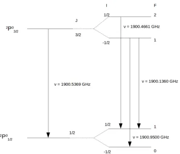
Figure 2.2: Fine-structure levels of C

⁺

and hyper-fine structure levels of

¹³

C

⁺

(see also Table 2.1).

low gas density. This makes collision unlikely, allowing the gas to decay by emitting a forbidden-line photon.

2.5.1 ¹² C ⁺ and ¹³ C ⁺ - Ionized Carbon

C

⁺

ground electronic state 1s

²

2s

²

2P

⁰

is divided into two fine-structure levels

²

P

⁰_1/2

and

²

P

⁰_3/2

, as we can see in Fig. 2.2. C

⁺

is excited to the

²

P

⁰_3/2

level through collisions with electrons (Keenan et al. 1986; Blum & Pradhan 1991; Wilson & Bell 2002; Wil- son et al. 2005), atomic hydrogen (Launay & Roueff 1977b; Barinovs et al. 2005) or molecular hydrogen (Flower & Launay 1977; Flower 1988), depending on whether the collision partner is available in the different layers of the PDR. The excitation is followed by a subsequent radiative decay to the

²

P

⁰_1/2

level by spontaneous emission or collisions, producing a photon of frequency 1900.5369 GHz or 157.7 µm (Cooksy et al. 1986), see table 2.1 for the [

¹²

CII ] spectroscopic parameters. [CII] fine structure line has a spontaneous emission probability of A

10

= 2.29 × 10

⁻⁶

s −1 (Mendoza 1983;

Tachiev & Froese Fischer 2001; Wiese & Fuhr 2007).

13

C

⁺

is one of the isotopes of C

⁺

. Due to the presence of an additional spin of

the unpaired neutron in the nucleus, the two C

⁺

fine-structure levels are splitted

into 4 hyper-fine structure levels, as we can see in Fig. 2.2. This hyper-fine split-

ting produces three components. These components are labeled by the total angular

momentum change F=2 → 1, F=1 → 0 and F=1 → 1. Figure 2.3 illustrates the resulting

spectrum for the case of a sufficiently narrow intrinsic line width, in such a way that

(27)

2.5. DESCRIPTION OF THE OBSERVED ATOMS AND MOLECULES

Figure 2.3: Spectral signature of the [

¹³

CII ] hyperfine structure and [

¹²

CII ] for a hypothetical, narrow line width (see also Table 2.1).

Table 2.1: [

¹²

CII ] and [

¹³

CII ] Spectroscopic parameters

Line Statistical Weight Frequency Vel. offset Relative

g

u

g

l

ν δ v

F→F⁰

intensity

(GHz) (km/s) s

F→F⁰

[

¹²

CII ]

²

P

3/2

−

²

P

1/2

4 2 1900.5369 0 −

[

¹³

CII] F=2→1 5 3 1900.4661 +11.2 0.625

[

¹³

CII] F=1 → 0 3 1 1900.9500 -65.2 0.250

[

¹³

CII ] F=1 → 1 3 3 1900.1360 +63.2 0.125

the strongest hyperfine satellite of [

¹³

CII], F=2→1, does not blend with the [

¹²

CII]

line. The frequencies of the hyper-fine transitions were determined by Cooksy et al.

(1986). Ossenkopf et al. (2013) confirmed that the hyper-fine frequencies were cor- rect through direct astronomical observations, with an accuracy of 3 MHz. They also computed the relative line strengths of the [

¹³

CII ] hyperfine satellites and noted that the relative strengths given by Cooksy et al. (1986) were incorrect. The right ratios for the F

⁰

− F = 2 − 1 : 1 − 0 : 1 − 1 transitions are 0.625:0.25:0.125, and the old line ratios were 0.444:0.356:0.20. This anomaly had also been reported before by Graf et al. (2012).

The relevant [

¹²

CII] and [

¹³

CII] spectroscopic parameters are summarized in Ta-

ble 2.1, including the velocity offsets of the [

¹³

CII] hyperfine components relative to

[

¹²

CII]. The frequency separation of the hyperfine lines is small enough that all lines

can be observed simultaneously with the bandwidth available in current, state-of-

the-art high resolution heterodyne receivers, the 130 km/s separation of the outer

hfs-satellites corresponds to slightly below 1 GHz frequency separation.

(28)

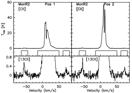
2.5.1.1 [CII] Optical Depth Estimation from the Main Beam Temperature ratio For a direct estimation of the optical depth from the observed main beam tempera- ture ratio, it can be assumed, as a first approximation, that the source is composed of a single, homogeneous layer. The optical depth is proportional to the line of sight integral of the population differences between the upper and lower states. We can estimate the ratio between the optical depth of [

¹³

CII ] and [

¹²

CII ] if two con- ditions are met: The chemical abundance ratio between

¹²

C

⁺

and

¹³

C

⁺

, defined as

12

C

⁺

/

¹³

C

⁺

=α

⁺

, is constant across the source; and the excitation temperature of the main isotopic line and all three [

¹³

CII] hyperfine satellites are identical at each posi- tion in the source.

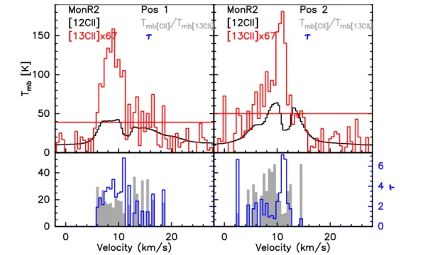
Instead of calculating the [

¹²

CII] optical depth for each [

¹³

CII] hyperfine satellite separately, the noise weighted average is used, of the appropriate velocity shifted and scaled-up three hyperfine satellites:

T

_mb,13,tot

(v) = P

F,F⁰

w

F→F⁰

T

_mb,13

(v − ∆v

F→F⁰

) s

F→F⁰

P

F,F⁰

w

_F→F⁰

w

_F_→F⁰

= s

F→F⁰

σ

2

(2.44)

with s

F→F⁰

the relative intensities from Table 2.1 and σ is the rms noise level of the observation. The F, F

⁰

-sum in eq. 2.44 runs over all satellites that are not blended with the main [

¹²

CII] line. From the radiative transfer equation from Eq. 4.13, the ratio between the temperatures of both isotopes can be expressed as:

T

_mb,12

(v)

T

_mb,13,tot

(v) = 1 − e

^−τ¹²^(v)

1 − e

^−τ^13,tot^(v)

(2.45)

Furthermore, the optical depth of [

¹³

CII] is inversely proportional to the abun- dance ratio α

⁺

as:

τ

_13,tot

(v) = β

_tot

τ

₁₂

(ν) (2.46)

β

_tot

= 1 α

⁺

X

F,F⁰

s

F→F⁰

(2.47)

If the three hyper-fine components are used β

_tot

= 1/α

⁺

, s

F→F⁰

is the relative

(29)

2.5. DESCRIPTION OF THE OBSERVED ATOMS AND MOLECULES

intensity of the [

¹³

CII] hyperfine satellite (Table 2.1). Combining Eq. 2.45 and 2.46, the [

¹²

CII] optical depth can be estimated as:

T

mb,12

(v)

T

_mb,13,tot

(v) ' 1 − e

^−τ(v¹²⁾

β

_tot

τ (v

₁₂

) (2.48)

2.5.1.2 [CII] Column Density and Optical Depth

For an atomic fine-structure level transition, the energy E

_i

is:

E

_i

= hν

_i

(2.49)

To estimate the [

¹²

CII ] column density, the partition function Z from Eq. 2.39 for a two level system is:

Z = g

_l

e

^−hν^l^/kT

+ g

_u

e

^−hν^u^/kT

(2.50)

And the optical depth from Eq. 2.43 becomes:

τ (v) = c

³

8πν

₀³

g

_u

g

_l

N A

_ul

"

1 − e

^−hν/kT

1 +

^g_g^u

l

e

^−hν^l^/kT

#

φ(v) (2.51)

From here, the column density can be derived from the integrated intensity. This is calculated from the integration of the main beam temperature from Eq. 4.13 de- fined below in Chapter 4, assuming that the background contribution is negligible and approximating the optical depth as (1-e

^−τ

) ≈ τ . Therefore, the integrated main beam temperature is:

Z

T

_mb

(v ) dv =

Z hν

₀

k

1 e

^hν⁰^/kT

− 1 τ (v) dv (2.52) and replacing Eq. 2.42 into 2.52:

Z

T

_mb

(v) dv = hν k

c

³

8πν

₀³

A

_ul

N 1 1 +

^g_g^u

l

e

^hν/kT

(2.53)

Rearranging Eq. 2.53 for the column density, becoming:

N (CII) = 8πkν

₀²

hc

³

A

_ul

f (T )

Z

T

_mb

(v) dv (2.54)

(30)

with f(T ) = 1 +

_g^g^l

u

e

^hν/kT

. In the high limit case for the temperature, if T goes to infinity, f(T) goes to 3/2. Higher values of f(T) occur at lower excitation tempera- tures. Therefore, a minimum column density can be defined for the high limit case as:

N

min

(CII) = 3 2

8πkν

₀²

hc

³

A

_ul

Z

T

mb

(v ) dv (2.55)

and the column density from Eq. 2.54 as:

N (CII) = 2

3 f(T ) N

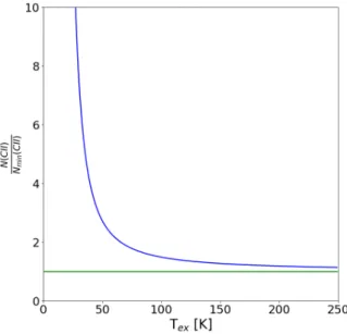
_min

(CII) (2.56) Figure 2.4 shows how the value of the excitation temperature affects the column density estimated from the integrated intensity, specially below the 91.2 K.

Figure 2.4: Ratio between N(CII) and N

min

(CII) as a function of the excitation tem- perature. Above the temperature of the [CII] transition, 91.2 K, the increase relative to the minimum value is well below a factor of 2.

2.5.2 C ⁰ - Neutral Carbon

Carbon ground electronic state is 1s

²

2s

²

2p

²

. The ground state is divided into three

fine-structure levels

³

P

0

,

³

P

1

and

³

P

2

(Saykally & Evenson 1980), see Fig. 2.5 for the

fine-structure level diagram.

(31)

2.5. DESCRIPTION OF THE OBSERVED ATOMS AND MOLECULES

Figure 2.5: Fine-structure levels of atomic carbon

It is excited mainly by collisions with atomic hydrogen (Yau & Dalgarno 1976;

Launay & Roueff 1977a; Abrahamsson et al. 2007), but also with He and H

2

(Mon- teiro & Flower 1987). [CI]

³

P

2

-

³

P

1

transition emits a photon with a frequency of 809.3 GHz and a spontaneous emission probability of A

21

= 2.68 × 10

⁻⁷

s −1 and

³

P

1

-

3

P

0

transition has a frequency of 492.2 GHz and a spontaneous emission probability of A

10

= 7.93 × 10

⁻⁸

s −1 (Draine 2011).

2.5.2.1 [CI] Column Density

From Gerin et al. (1998), the neutral carbon column density, under LTE conditions, is:

N (C) = 1.9 × 10

¹⁵

Z

T

_mb

dv Q(T

_kin

)e

^E¹^/kT^kin

(cm

⁻²

) (2.57)

with the partition function Q(T ) = 1 + 3e

^−E¹^/kT

+ 5e

^−E²^/kT

, carbon atom energy

levels E

₁

/k = 23.6 K and E

₂

/k = 62.5 K, the integrated intensity in units of K km

s

⁻¹

and T

_kin

the kinetic temperature of the carbon gas.

(32)

2.5.3 N ⁺ - Ionized Nitrogen

N

⁺

corresponds to ionized nitrogen. The atom has an ionization potential of 14.5 eV, higher than hydrogen. For this reason, it can be found in HII regions and in diffuse ionized gas, tracing the ionized hydrogen and reflecting the effects of the UV pho- tons, as well as the electron density. N

⁺

is created mainly by UV photoionization, but also by cosmic rays and x-rays ionization, electron collisional excitation and pro- ton charge exchange (Langer et al. 2015). It is depleted in fully ionized regions by electron radiative and dielectronic recombination, and in partially ionized regions also by exothermic charge exchange with atoms.

Figure 2.6: Fine-structure levels of ionized nitrogen N

⁺

N

⁺

in the ground electronic state is distributed as 1s

²

2s

²

2p

²

. Due to its electronic distribution, it is divided in three fine structure levels, similar to neutral carbon.

³

P

2

has a E

j

/k of 118 K with a g

2

= 5,

³

P

1

has a E

j

/k of 70 K with a g

1

= 3 and

³

P

0

has a

E

j

/k of 0 K with a g

0

= 1. [NII]

³

P

2

-

³

P

1

transition has a frequency of 2459.371 GHz

(121.9 µm), meanwhile

³

P

1

-

³

P

0

transition has a frequency of 1461.134 GHz (205.2

µ m) (Brown et al. 1994). The spontaneous emission probability A

21

corresponds to

7.5 × 10

⁻⁶

s −1 and A

10

to 2.1 × 10

⁻⁶

s −1 (Galavis et al. 1997). It is excited through

collision with electrons (Lennon & Burke 1994; Hudson & Bell 2004; Tayal 2011).

(33)

2.5. DESCRIPTION OF THE OBSERVED ATOMS AND MOLECULES

2.5.3.1 [NII] Column Density

From Langer et al. (2015), the [NII] column density can be estimated from the inte- grated intensity in the optically thin limit as:

I

_ul

([NII]) = Z

T (K) dv = hc

³

8πν

_ul²

A

_ul

f

_u

N (N

⁺

) (2.58) where A

_ul

is the Einstein A coefficient for the transition, ν

_ul

the transition fre- quency, f

_u

is the fractional population of the upper state, N (N

⁺

) is the column den- sity and the integrated intensity is in units of K km s

⁻

1. For the 205 µm

³

P

1

-

³

P

0

transition, it can be written as (Langer et al. 2015):

I

ul

([NII]) = 5.06 × 10

⁻¹⁶

f

1

N (N

⁺

) (K km s

⁻

1) (2.59)

with f

₁

fractional population of N

⁺

in the

³

P

1

state. The fractional population has the condition of f

₂

+ f

₁

+ f

₀

= 1, with f

_i

the fractional population of the different levels. N

⁺

is excited by electron collision, therefore, the level populations depend directly from the electron density of the HII region. From Goldsmith et al. (2015), Fig. 2.7 shows how the population fraction for the different levels changes for a ki- netic temperature of 8000 K.

If only the

³

P

1

-

³

P

0

transition has been observed, it is not possible to derive the electron density. But assuming a kinetic temperature of 8000 K, the population frac- tion of the level

³

P

1

peaks at 0.45 with an electron density of 100 cm

⁻³

. Therefore, this value can be used to derive the column density as a lower limit.

2.5.4 CO - Carbon Monoxide Rotational Transitions

CO, carbon monoxide is a diatomic heteronuclear molecule. Diatomic molecules correspond to molecules formed by two atoms. Each electronic state can be defined by a vibrational quantum number v and a rotational quantum number J , that cor- responds to the total angular momentum, that is the sum of the electronic angular momentum L and the angular momentum N . Heteronuclear diatomic molecules are molecules formed by different atoms, such as CO, OH or HD. They have a per- manent electric dipole, hence vibrational and rotational transitions are allowed in the ground electronic state. The spontaneous emission coefficient A

_ul

is given by (Mangum & Shirley 2015):

A

_ul

= 64π

⁴

ν

³

3hc

³

|µ

_lu

|

²

(2.60)

(34)

Figure 2.7: Fractional populations of three N

⁺

fine structure levels for kinetic tem- perature of 8000 K, as a function of electron density. From Goldsmith et al. (2015)

with |µ

lu

|

²

the dipole matrix element. For a pure rotational transition in the ground electric and vibrational levels, from J to J -1, the dipole matrix element is:

|µ

_lu

|

²

= µ

²

J

2J + 1 J → J − 1 (2.61)

with µ

²

the permanent electric dipole moment of the molecule. The energy levels for the rotational transitions, using the rigid rotor approximation, are:

E

_J

= hB

₀

J (J + 1) (2.62)

with B

0

the rigid rotor rotation constant. The partition function Z from Eq. 2.39 can be approximated for a diatomic molecule as (Schneider et al. 2016b):

Z

_mol

=

∞

X

J=1

(2J + 1)e

−EJ

kB T

∼ k

_B

T

_ex

hB

0

+ 1/3 (2.63)

CO has a permanent dipole moment of µ ≈ 0.11 × 10

⁻¹⁸

esu cm, the ground rota-

tional transition has rotational frequency B = ν /2/J, h

²

/I k ≈ 5.5 K and a critical den-

sity of 2200 cm

⁻³

. The combination of these three conditions results in the CO being

(35)

2.5. DESCRIPTION OF THE OBSERVED ATOMS AND MOLECULES

easily excited, even in cold molecular clouds. CO is excited mainly through collision with H

2

and by radiative trapping (Scoville & Solomon 1974; Green & Thaddeus 1976). Radiative trapping means that the emission of excited CO is reabsorbed by an unexcited one, trapping the photons inside the cloud at large optical depths.

Also, the beam average total column density can be determined from the ob- served integrated main beam intensity as (Schneider et al. 2016b):

N = 3hZ

_mol

8π

³

µ

²

J

e

^E^J^/kT^ex

[1 − e

^−hν/kT^ex

](J(T

ex

) − J(T

BG

)) Z

T

_mb

dv (cm

⁻²

) (2.64)

with J (T ) the brightness temperature from Eq. 2.8, T

_BG

= 2.7 K, J the upper rota- tional quantum number value of the transition and R

T

_mb

dv the velocity integrated

line intensity in units of K km s

⁻¹

.

(36)

(37)

3 | Astrophysics

In this chapter, there is a discussion of the characteristics of the Photodissociation Regions, such as physical and chemical processes, regions that are part of them and the main atoms and molecules that form the gas on them. This description is a gen- eral review about this kind of regions and serves as an introduction to the subject.

For more in-depth reviews, readers are invited to check artciles such as Photodissoci- ation regions. I - Basic model. II - A model for the Orion photodissociation region (Tielens

& Hollenbach 1985), Dense Photodissociation Regions (PDRs) (Hollenbach & Tielens 1997) and Photodissociation Regions in the Interstellar Medium of Galaxies (Hollenbach

& Tielens 1999). There is a discussion also about the origin of the

¹²

C/

¹³

C Isotopic Abundance Ratio and how it changes across the Galaxy. Finally, a description is given of the four PDR sources observed for this thesis work: M43, the Horsehead PDR, Monoceros R2 and M17. Their physical characteristics and observations that have been done before this work are described below.

3.1 Photodissociation Regions

A Photodissociation Region (PDR) is a region of the interstellar medium (ISM) where the structure, thermal balance and chemistry are dominated by Far-UV (FUV) pho- tons that interact with the gas and dust of the region. The PDR is a transition region between the fully ionized to the dense molecular gas. The FUV photons are gener- ated by nearby OB stars and they have energies between 6 eV and 13.6 eV (Tielens &

Hollenbach 1985; Hollenbach & Tielens 1997, 1999). At lower energies, most atoms are not ionized and photoelectric in dust grains is negligible. At higher energies, hy- drogen is ionized and it is not part of a PDR. The FUV average interstellar radiation is usually expressed in terms of the Habing field (Habing 1968) corresponding to:

G

₀

≡ u(6 − 13.6 eV )

5.29 × 10

⁻¹⁴

erg cm

⁻³

(3.1)

with u(6-13.6 eV) the energy density between 6 and 13.6 eV. It can be expressed

also in Draine units (Draine 1978), with χ = 1.71 G

₀

. The incident flux for a PDR

(38)

ranges from the local average interstellar radiation field (ISRF) of 1.7 G

0

(Draine 1978), which contains contributions from early-type stars from the Galaxy, to G

0

≥ 10

⁶

.

The incident FUV field photodissociates molecules, photoionizes atoms and molecules and heats the gas and dust through photoelectric heating or direct absorption of photons. These mechanisms produce a layered structure, as shown in Fig. 3.1. As- suming that the incident FUV flux comes from the left, and going deeper into the cloud from left to right, the column density progressively increases and the tempera- ture of the gas and dust decrease. Outside the PDR, there is the so-called HII region, where hydrogen is ionized by the incident FUV field, with gas temperatures ∼ 10

⁴

K and visual extinction (A

v

) lower than 0.1 magnitudes. Due to the photoionization of hydrogen, all the photons with energy higher than 13.6 eV are absorbed, creating an ionization front, separating the HII region from the PDR itself and forming a layered structure. Additionally, species with a ionization potential higher than hydrogen be- come completely neutral inside the PDR, such as nitrogen (14.5 eV) or oxygen (13.6 eV), and species with a ionization potential lower than H are photoionized inside the PDR, such as carbon (11.3 eV).

3.1.1 H/H 2 Transition Zone

Thus, inside the PDR, the gas temperature in the outer layers ranges from 10

²

to 10

³

K. The abundance of atomic hydrogen is kept in equilibrium between the reduction of atomic hydrogen through the formation of molecular hydrogen (H

2

) on the sur- face of dust grains, and the increase of it through the photodissociation of H

2

by the absorption of FUV photons in the Lyman and Werner transitions in the 912 to 1100 Å wavelength range, pumping H

₂

to a bound excited electronic state. This absorp- tion is followed by fluorescence back to an excited vibrational state in the ground electronic state, and leads to dissociation only 10% of the time. The electronic ex- cited H

2

dissociates through reactions with atoms such as C

⁺

or O or collisions with H or H

2

to overcome the activation barrier and fluorescence back to the vibrational continuum and then dissociate.

When the molecular hydrogen column density increases (> 10

¹⁴

cm

⁻²

), H

2

be- comes optically thick and self-shields Lyman and Werner transitions. This allows for an increase of H

2

, helped by the progressive attenuation of the FUV radiation by dust grains. Therefore, the photodissociation rate depends on the H

2

abundance and level population as a function of the depth in the cloud. Therefore, an H/H

2

transition zone or dissociation front appears, with a sharp profile at A

v