Molecular Cloud Structure in the Star-forming Region W43

Molecular Cloud Structure in the Star-forming Region W43

Inaugural-Dissertation

zur

Erlangung des Doktorgrades

der Mathematisch-Naturwisschenschaftlichen Fakultät der Universität zu Köln

vorgelegt von

Philipp Christoph Carlhoff aus Krefeld

Köln 2013

Prof. Dr. Jürgen Stutzki

Tag der mündlichen Prüfung: 16. Januar 2014

Für Flora

“The world is full of magical things patiently waiting for our wits to grow sharper.”

Bertrand Russell

Abstract

In the struggle toward an understanding of the process of star formation it is one of the most important tasks to study the initial properties of the cold and dense interstellar medium. Stars are known to form in dense molecular clouds, but it is not yet fully understood how they from from the neutral gas that permeates the Galaxy. Therefore, it is crucial to fully understand the creation process of molecular clouds.

Colliding flows are a possible explanation for this process. This class of mod- els considers streams of warm, diffuse, and atomic hydrogen gas that stream into each other. Fluctuations of the gas at the collision area create regions of higher density and lower temperature, where molecules can form.

W43 is one of the largest molecular cloud complexes in the Milky Way with a total gas mass of several 10

M . Prior investigations have identified it as one of the largest and most luminous star-forming regions in the Galaxy. This is most probably due to its exceptional position, which is assumed to be at the junction point of the Galactic spiral arms and the bar. At this location, gas is piled up, because the elliptical orbits in the bar and the circular orbits in the spiral arms interfere. Therefore, W43 poses an excellent laboratory to study the formation of molecular clouds.

This thesis aims at characterizing the W43 star-forming region. The distri- bution of molecular clouds, their velocity structure, and physical properties are analyzed and the origin of a single filament is studied in detail.

The first part of this work describes the project W43 HERO (W43 Hera/EmiR Observations) that has been initiated to observe the large scale distribution of

13

CO (2–1) and C

O (2–1) in the W43 complex with the IRAM 30m telescope.

These molecular emission lines provide information of the medium dense molec- ular gas (n ≈ 10

cm

) in the complex. While

CO (2–1) traces the more dif- fuse, widespread gas in the clouds, C

O (2–1) is used to depict the denser central clumps of the clouds.

We analyze the velocity structure of our data and align our findings with ve- locity models of the spiral arms in the Galaxy. We thus confirm the position of W43 near the tangential point in the Scutum arm, which is situated near the tip of the elongated bar. This point has a distance of 6 kpc from the Sun.

v

We then derive the optical depth, the excitation temperature, and the H

col- umn density of the gas from our observations. The total mass of medium dense molecular clouds in the W43 complex is found to be 1.9 × 10

M . An estima- tion of the shear parameter of the cloud complex provides the insight that it is massive enough to withstand the shear forces generated by the motions of gas streams in the Galaxy. Mass estimations are in agreement with those taken from Herschel dust emission maps.

Plots of the probability distribution functions of the H

column density, derived from Herschel and the IRAM 30m data, are created. Both show a log-normal distribution on lower masses and power-law deviation on the high-mass end of the function. This is commonly associated with the influence of star formation.

The slope of the CO power-law tail is less steep than that derived from dust emission. We could have found an efficient tool, that only traces the gas that collapses into a protostar.

In the second part of this thesis we pick one single filament in the W43 complex and analyze it in detail. Additional observations have been carried out to complement the IRAM 30m dataset. In particular, there are observa- tions of CO (6–5) from the APEX telescope, [C II] from the Herschel satellite, [C I], observed with NANTEN2, and the CARMA observations of HCN (1–0), HCO

(1–0), and N

H

(1–0).

We use the radiative transfer code RADEX to estimate the temperature and density of the molecular gas. The best solution is a kinetic temperature around 30 K and a density of ∼ 10

cm

. We then study the origin of the ionized carbon which we have observed with Herschel. This species is often discussed in the framework of static photon-dominated regions (PDRs). The physical conditions are studied with the program KOSMA-τ , which yields a very high UV-field, neces- sary for the creation of the observed data. A comparison with typical UV-tracers results in the insight that this radiation strength is unrealistically high. Thus, the creation of C

by a static PDR is implausible and a different mechanism has to be the origin.

We find it more likely that the [C II] emission traces the transition zone be- tween the initial atomic gas and the molecular cloud which forms from it. We would thus witness the dynamic formation of a young molecular filament.

We conclude that W43 is indeed one of the most massive and important

molecular cloud complexes in the Galaxy and that colliding flows are a possible

explanation for its formation.

Zusammenfassung

Den Ausgangszustand des kalten, dichten interstellaren Mediums zu verstehen ist einer der wichtigsten Aspekte, um den Prozess der Sternentstehung zu er- klären. Es ist bekannt, dass Sterne in dichten Molekülwolken entstehen, es ist jedoch noch nicht vollständig verstanden, wie diese aus dem neutralen Gas, das die Galaxie durchdringt, entstehen. Deshalb ist es entscheidend, den Ent- stehungsprozess dieser Molekülwolken nachzuvollziehen.

Kollidierende Gasströme sind eine mögliche Erklärung dieses Prozesses.

Diese Klasse von Modellen betrachtet Ströme warmen, diffusen, atomaren Was- serstoffgases, die ineinander fließen. Fluktuationen des Gases innerhalb der Kollisionsfläche erzeugen Regionen erhöhter Dichte und niedrigerer Tempera- tur, in denen Moleküle enstehen können.

W43 ist einer der größten molekularen Wolkenkomplexe in der Milchstra- ße mit einer Gesamtmasse von mehreren 10

M . Vorausgehende Untersu- chungen haben es als eine der größten und leuchtkräftigsten Sternenstehungs- regionen in der Galaxie identifiziert. Der Grund dafür ist wahrscheinlich die au- ßergewöhnliche Position, welche am Treffpunkt der galaktischen Spiralarme und dem Balken vermutet wurde. Da sich dort die elliptischen Orbits des Balkens und die kreisförmigen Orbits in den Spiralarmen überlagern, wird an diesem Punkt Gas angehäuft. Daher bietet W43 exzellente Bedingungen, um die Entstehung von Molekülwolken zu studieren.

Ziel dieser Arbeit ist es, die Sternenstehungsregion W43 zu charakterisie- ren. Die Verteilung der Molekülwolken, ihre Geschwindigkeitsstruktur und phy- sikalischen Eigenschaften werden analysiert und der Ursprung eines einzelnen Filaments genauer untersucht.

Der erste Teil dieser Arbeit beschreibt das Project W43 HERO (W43 He- ra/EmiR Observations), das begonnen wurde, um die Verteilung von

CO (2–1) und C

O (2–1) im W43 Komplex mit dem IRAM 30m Teleskop zu beobachten.

Diese Molekülemissionslinien liefern Informationen über das molekulare Gas mittlerer Dichte (n ≈ 10

cm

) im Komplex. Das weiter ausgedehnte, diffusere Gas wird durch

CO (2–1) beobachtet, wohingegen C

O (2–1) genutzt wird um die etwas dichteren, zentralen Klumpen innerhalb der Wolken darzustellen.

Wir analysieren die Geschwindigkeitsstruktur unserer Daten und vergleichen unsere Ergebnisse mit Geschwindigkeitsmodellen der Spiralarme in der Galaxie.

vii

Auf diese Weise können wir die Position von W43 in der Nähe des Tangential- punktes im Scutum-Arm bestätigen, welcher sich nahe der Spitze des verlän- gerten Balkens befindet. Dieser Punkt hat eine Entfernung zur Sonne von 6 kpc.

Wir leiten danach die optische Tiefe, die Anregungstemperatur und die H

Säulendichte des Gases von unseren Beobachtungen ab. Die Gesamtmasse des molekularen Gases mittlerer Dichte im W43 Komplex beträgt 1.9 × 10

M . Eine Abschätzung des Scherungs-Parameters der Wolke erlaubt die Einsicht, dass diese massereich genug ist, um den Scherkräften zu widerstehen, wel- che durch die Bewegung der Gasströme in der Galaxie erzeugt werden. Die Masseschätzung stimmt mit den Werten überein, die wir aus Herschel Staub- emissionskarten erhalten haben.

Abbildungen der Wahrscheinlichkeitsverteilungsfunktionen der H

Säulen- dichte, abgeleitet von Herschel und IRAM 30m Daten, werden erzeugt. Beide zeigen eine logarithmische Normalverteilung bei niedrigen Massen und eine Ab- weichung in Form eines Potenzgesetzes bei hohen Massen. Dies wird norma- lerweise mit dem Einfluss der Sternenstehung in Verbindung gebracht. Die Stei- gung des CO Potenzgesetzes ist weniger steil als diejenige, die aus der Staub- emission abgeleitet wurde. Möglicherweise haben wir eine effiziente Methode gefunden, nur jenes Gas zu erkennen, welches zu einem Protostern kollabiert.

Im zweiten Teil der Arbeit suchen wir ein spezielles Filament im W43 Kom- plex heraus und analysieren es im Detail. Zusätzliche Beobachtungen wurden durchgeführt, um das IRAM 30m Datenset zu vervollständigen. Im Einzelnen sind dies Beobachtungen von CO (6–5) mit dem APEX Teleskop, [C II] vom Her- schel Satelliten, [C I], beobachtet mit NANTEN2 und die CARMA Beobachtun- gen von HCN (1–0), HCO

(1–0) und N

H

(1–0).

Wir verwenden den Strahlungstransportcode RADEX, um die Temperatur und Dichte des molekularen Gases zu bestimmen. Die besten Lösungen sind eine kinetische Temperatur von etwa 30 K und eine Dichte von ∼ 10

cm

. Daraufhin analysieren wir den ionisierten Kohlenstoff, welchen wir mit Her- schel beobachtet haben. Dieses Element wird häufig im Rahmen von statischen photonendominierten Regionen (PDRs) diskutiert. Die physikalischen Bedin- gungen werden mit dem KOSMA-τ -Programm untersucht, welches ergibt, dass ein sehr starkes UV-Feld nötig wäre, um die beobachteten Daten zu erzeugen.

Ein Vergleich mit typischen UV-Tracern zeigt, dass dieses Strahlungsfeld un- realistisch stark ist. Daher ist die Erzeugung von C

durch eine statische PDR unplausibel und ein anderer Mechanismus muss als Ursprung dienen.

Es erscheint uns wahrscheinlicher, dass die [C II] Strahlung die Übergangs- zone markiert, welche zwischen urpsrünglichem atomarem Gas und der Mole- külwolke, welche sich daraus entwickelt, befindet. Somit würden wir Zeuge der dynamischen Entstehung eines jungen molekularen Filaments.

Wir schließen, dass W43 in der Tat einer der massereichsten und wichtigsten

Molekülwolkenkomplexe in der Galaxie ist und eine mögliche Erklärung seiner

Entstehung in der Theorie kollidierender Gasströme zu finden ist.

Contents

1 Introduction 1

1.1 Structure of this work . . . . 3

2 Theoretical backgrounds 5 2.1 Astrophysical backgrounds . . . . 5

2.1.1 Star formation . . . . 5

2.1.2 Interstellar medium . . . . 11

2.1.3 Molecular cloud formation . . . . 13

2.1.4 Filamentary structure . . . . 15

2.1.5 Structure of the Milky Way . . . . 17

2.1.6 The W43 star-forming region . . . . 19

2.2 Submm/mm-Astronomy . . . . 20

2.2.1 Radio telescopes . . . . 21

2.2.2 Receivers used in radio astronomy . . . . 22

2.2.3 Interferometer telescopes . . . . 24

2.2.4 Molecular emission lines . . . . 24

2.2.5 Fine-/Hyperfine structure lines . . . . 27

2.2.6 Line profile and Doppler effect . . . . 28

3 Large scale CO observations of W43 31 3.1 Contribution of co-authors . . . . 31

3.2 The observations . . . . 32

3.2.1 Observed lines . . . . 32

3.2.2 The IRAM 30m telescope . . . . 32

ix

3.2.3 Telescope setup . . . . 33

3.2.4 Data reduction . . . . 35

3.3 Noise maps . . . . 36

3.4 Results . . . . 37

4 Velocity structure of W43 41 4.1 Average spectra . . . . 41

4.2 Decomposition into sub-cubes . . . . 41

4.2.1 GAUSSCLUMPS decomposition . . . . 43

4.2.2 Duchamp Sourcefinder decomposition . . . . 44

4.2.3 Naming conventions . . . . 46

4.3 PV-Diagram of the region . . . . 47

4.4 Determination of the distance of W43 . . . . 49

4.5 Mean velocity and line width . . . . 53

4.6 Moment maps of foreground components . . . . 54

5 Physical properties of molecular clouds in W43 57 5.1 Derived properties . . . . 57

5.1.1 Optical depth . . . . 57

5.1.2 Excitation temperature . . . . 59

5.1.3 H

column density . . . . 62

5.1.4 Total mass . . . . 64

5.2 Shear parameter . . . . 66

5.3 Virial masses . . . . 68

5.4 Larson’s laws . . . . 69

5.5 Comparison to other projects . . . . 70

5.5.1 Spitzer GLIMPSE and MIPSGAL . . . . 71

5.5.2 APEX ATLASGAL . . . . 73

5.5.3 VLA THOR project . . . . 73

5.5.4 Herschel Hi-GAL . . . . 74

5.6 Column density probability distribution function . . . . 78

5.7 Description of W43-Main and W43-South . . . . 80

5.7.1 W43-Main, Source 13 . . . . 81

5.7.2 W43-South, Source 20 . . . . 84

CONTENTS xi 6 Detailed observations of a filament in W43 87

6.1 Herschel [C II] observations . . . . 87

6.1.1 The Herschel Space Observatory . . . . 88

6.1.2 The HIFI instrument . . . . 89

6.1.3 The [C II] emission line . . . . 90

6.1.4 Telescope setup . . . . 90

6.1.5 Data reduction . . . . 91

6.1.6 Resulting map . . . . 91

6.2 APEX CO observations . . . . 92

6.2.1 The APEX telescope . . . . 92

6.2.2 Telescope setup . . . . 93

6.2.3 Data reduction . . . . 93

6.2.4 Resulting map . . . . 94

6.3 CARMA high-density tracers observations . . . . 94

6.3.1 The CARMA interferometer . . . . 94

6.3.2 Description of the observed lines . . . . 95

6.3.3 Telescope setup . . . . 96

6.3.4 Data reduction . . . . 96

6.3.5 Resulting maps . . . . 98

6.3.6 Observations of a second filament . . . . 99

6.4 NANTEN2 [C I] observations . . . . 99

6.4.1 The NANTEN2 telescope . . . . 99

6.4.2 The [C I] emission line . . . . 100

6.4.3 Telescope setup . . . . 100

6.4.4 Data reduction . . . . 100

6.4.5 Resulting map . . . . 101

6.5 SMA CO observations . . . . 103

6.6 Overview . . . . 103

7 Analysis of a filament in W43 105

7.1 Spatial and spectral analysis . . . . 105

7.1.1 Herschel data . . . . 105

7.1.2 APEX data . . . . 108

7.1.3 CARMA data . . . . 109

7.1.4 NANTEN2 data . . . . 113

7.1.5 Filament shape and size . . . . 115

7.1.6 Example spectra . . . . 116

7.2 Properties of the filament . . . . 118

7.2.1 Temperature and density . . . . 118

Naive density estimation . . . . 118

The RADEX algorithm . . . . 119

RADEX results . . . . 120

CARMA data density estimation . . . . 123

7.2.2 UV-field . . . . 124

C

in PDRs . . . . 124

The KOSMA-τ model . . . . 125

KOSMA-τ results . . . . 126

Comparison with UV-field tracers . . . . 128

7.2.3 Origin of C

in the filament . . . . 132

8 Summary and Conclusion 135 8.1 Summary . . . . 135

8.1.1 Analysis of the large scale structure of the W43 complex . 135 8.1.2 Analysis of a single filament in W43 . . . . 137

8.2 Conclusion . . . . 138

8.3 Outlook . . . . 140

References 143

CONTENTS xiii

A Description of important sources 153

A.1 Source 23 . . . . 153

A.2 Source 25 . . . . 154

A.3 Source 26 . . . . 154

A.4 Source 28 . . . . 155

A.5 Source 29 . . . . 156

B Plots of all sources 157

List of Figures 187

List of Tables 191

List of Acronyms 193

List of Constants and Units 197

List of Publications 199

Acknowledgements 201

Erklärung 203

Chapter 1

Introduction

Throughout the history of mankind, observations of the sky have played an im- portant role. Even the earliest human tribes used the stars for navigation, cal- culation of times, and an inspiration for their mythology. When humanity started to became agricultural, determining times from observations of the sun and the nightly sky became so important, that it got a central part of everyday life in form of holidays, rites, and traditions. Astronomy can thus be considered one of the first sciences (although we cannot use this word in its modern meaning).

For millennia, people could only use their eyes to watch the sky. And al- though great progress was made in the description of planets, stars, comets, and nebulae, this covered only a fraction of the information that is transported to us through space. Even with the invention of the first lenses and telescopes, that drastically improved the accuracy of observations, still, only the visible light was accessible to us.

Only in the 19th century, the works of Maxwell (1873) made clear that light had to be considered as an electromagnetic wave and that it was only a small window of the complete electromagnetic spectrum. These electromagnetic waves were discovered by Hertz (1887) with his newly built antennas. The unit of frequency, in oscillations per second, was named after him. The first actual astronomical observations in the radio wavelengths were conducted by Jansky (1933), operating at wavelengths of 14.6 m. Astronomers discovered that these wavelengths (and others, up to the infrared regime) mainly trace the interstellar medium (ISM), clouds of gas and dust that fill the space between the stars.

Many processes in the ISM can be studied with the help of radiation in the millimeter and sub-millimeter wavelengths (several ten µm to a few mm). In- strumentation of telescopes for this range is not only technically demanding, but includes fundamentals of physics that are just about to be understood. This is the reason this field has flourished only in the last decades. With better re- ceivers and more computing power, larger and more detailed maps with higher spectral resolution became possible, fueling increasing insight into the physical

1

processes. Figure 1.1 shows the Atacama Large Millimeter/submillimeter Array (ALMA), the newest and most advanced interferometer, which operates in the submm/mm range.

Over the time, a completely new astronomical field was established, the study of the ISM and the process of star formation. This process is not only interesting by itself, but also has an important impact on the ISM through feedback effects.

Stars were found to emerge from molecular gas clouds (e.g. McKee and Ostriker 2007). They have to be cold and dense for stars to be able to form. Until today, it is not fully understood how these clouds develop, as the initial gas in the Galaxy is warm and atomic. The process of molecular cloud formation is therefore one of the crucial recent subjects of investigation in radio astronomy.

Fig. 1.1: Night sky over the ALMA telescope in the Atacama desert, Chile. Credits of image: C. Malin, European Southern Observatory (ESO).

To understand this formation process, the structure of giant molecular clouds (GMCs) needs to be studied. It was found that these molecular clouds show a fractal distribution of gas over several orders of magnitude (Stutzki et al. 1998).

Theoretical models and recent observations show that filamentary shapes form at certain scales and that star-forming cores grow along these filaments (e.g.

Banerjee et al. 2009; André et al. 2010). It is therefore important to analyze the mechanisms that create them. Especially, the transition phase between atomic and molecular clouds requires attention.

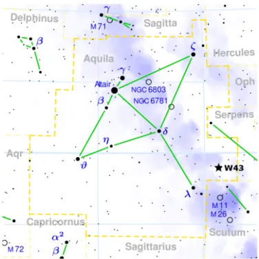
One of the most prominent star-forming regions in our Galaxy, besides the Galactic center, is the GMC W43. This region is located in the Galactic plane at 30

Galactic longitude, in the constellation Aquila. Figure 1.2 shows the position of W43 on the sky. This region was identified as one of the most massive and most luminous cloud complexes in the Galactic plane by Nguyen Luong et al.

(2011). It harbors a cluster of OB-stars that recently formed in this region and

fuels further star formation. W43 is assumed to be located at the junction point

1.1. STRUCTURE OF THIS WORK 3

Fig. 1.2: Position of W43 in the Aquila constellation. Credits of image: Wikipedia.org.

of the Galactic spiral arms and the bar, which is a distinguished position in the Galaxy, where different classes of orbits intersect and colliding mass is piled up.

The goal of this thesis is to characterize the molecular clouds located in the star-forming region W43 and clarify the process of their formation. Large scale maps of the medium density molecular clouds in W43, observed with the IRAM 30m, are described and analyzed. We study the velocity structure of this cloud complex and determine its physical properties. One single filament is then investigated in more detail.

Observations of ionized and atomic carbon as well as high-density tracers are presented. They allow to characterize the transition zone between atomic and molecular clouds. We study the origin of the ionized carbon emission and try to find out whether it has a dynamic origin. This would be a hint at the dynamic formation process of this filament.

1.1 Structure of this work

We now give a short overview of the structure of this thesis. After this intro-

duction, in chapter 2, we explain some theoretical backgrounds, needed for our

project. Star and molecular cloud formation are discussed in Sect. 2.1.1 and

2.1.3. The spiral arm structure of the Milky Way is explained in Sect. 2.1.5, while

Sect. 2.1.6 introduces the W43 molecular cloud complex and gives an overview

of previous research related to it. Finally, some technical descriptions of astro- nomical observation fundamentals are given in Sect. 2.2.

The project itself consists of two main parts, the large scale CO observations of the W43 complex and their analysis and the detailed small scale investigation of one filament, using complementary observations. Chapter 3 describes the CO observations, taken with the 30m telescope that is operated by the Institut de Radioastronomie Millimétrique (IRAM), while in chapter 4 we analyze the velocity structure of the CO dataset and describe the position of W43 in the Galaxy. We then derive physical properties of the W43 region in chapter 5 and compare our data to far-infrared and submillimeter dust emission maps. Is there any similarity between molecular line emission and dust continuum maps? The findings of these three chapters have been published in Carlhoff et al. (2013).

From this dataset we then choose one filament and analyze it in detail. Chap- ter 6 gives an overview of the additional observations with the Herschel Space Observatory (HSO), the Atacama Pathfinder Experiment (APEX), the Combined Array for Research in Millimeter-wave Astronomy (CARMA), and NANTEN2. The information gathered from these datasets is then given in chapter 7, where, apart from the exact size and velocity structure of the filament, we determine its tem- perature and density. We finally investigate the origin of ionized carbon emis- sion. Is the filament a typical photodissociation region/photon-dominated region (PDR) or do we need a different explanation? And what does this reveal about the transition phase between atomic and molecular gas?

To finish the thesis, a summary and conclusion of the results is given in

chapter 8. It also contains an outlook on open questions and possibilities for

future research. A short description of several important sources can be found

in Appendix A, while plots of all sources are shown in Appendix B.

Chapter 2

Theoretical backgrounds

In this chapter, we discuss some of the astrophysical fundamentals that pose the physical background of this work. In section 2.1 we give a short introduc- tion to the theory of star formation, which role molecular clouds play, and how they form. We give an overview of the Galactic structure and introduce the W43 star-forming region. Then, we want to describe some technical details of astro- nomical observations that were used during the data collection for this project.

Basics of single-dish and interferometer telescopes are explained in Sect. 2.2 together with the background of molecular emission lines that are used to study the properties of the ISM.

2.1 Astrophysical backgrounds

2.1.1 Star formation

Star formation is one of the most important processes in Galaxies. At this point, we explain the basics of this process as it strongly influences the energy balance of the ISM on all scales through feedback effects. Especially the formation of high-mass stars (M & 8 M ) has a crucial impact on its surroundings and is thus relevant for this thesis. Although many steps of the formation process are understood by now (McKee and Ostriker (2007) give a good overview), there are still important open questions.

It has been known for a long time that the formation processes of high- and low-mass stars differ strongly (Herbig 1962). These two types of stars are distin- guished by the Kelvin-Helmholtz timescale

τ

= G M

R L , (2.1)

5

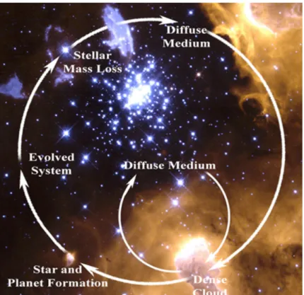
Fig. 2.1: Cycle of star formation. Credits: National Aeronautics and Space Administration (NASA).

where M , R, and L are the mass, radius, and luminosity of the star, respectively.

It denotes the time needed for gravitational collapse of the star, decelerated by its radiation. The formation of low-mass stars takes on the order of τ

, while the formation of high-mass stars takes longer.

Mezger and Smith (1977) noted that high-mass and low-mass stars seem to form in different locations. OB stars (hot and luminous high mass stars) primar- ily form in molecular clouds complexes of large masses. These complexes are called GMCs and are usually found in the spiral arms of Galaxies. Although they only take up a small part of the volume of the ISM, GMCs contain an important part of the total molecular gas mass. Individual cloud complexes show masses of at least 10

M , but are usually on the order of 10

–10

M (Williams et al.

2000). We discuss the formation of these molecular clouds in Sect. 2.1.3.

The final mass of the formed star depends strongly on the mass of the initial

cores. As usually groups of stars form in the same region, it is possible to mea-

sure the distribution of these stars. This initial mass function (IMF) measures

the mass of the stars at the point where they enter the main sequence and is

usually given as a probability distribution function (PDF). The IMF has first been

2.1. ASTROPHYSICAL BACKGROUNDS 7 described by Salpeter (1955) and has the characteristic form

ξ(m)∆m = ξ

m

M

∆m M

, (2.2)

where ξ(m)∆m is the number of stars with masses between m and m+∆m. This function ranges to a maximum stellar mass of 10 M . It has later been refined by Kroupa (2001), who introduced an IMF that shows a turnover at low masses (cf.

dot-dashed line in Fig. 2.2) and Chabrier (2003), who used a smoother function (cf. dashed line in Fig 2.2).

Inside the molecular clouds, regions of higher density lead to the formation of cores. Cores are defined to be smaller, colder, and denser regions of molec- ular clouds that are gravitationally bound. Typically, their size ranges from below 0.1 pc to nearly 1 pc, having a temperature between 10 and 15 K and masses of a few to a few hundred M (Benson and Myers 1989). Assuming a uniform, stationary, isothermal gas with perturbations of length scale λ, these are stable if the thermal energy of the gas can balance its gravity. Jeans instability occurs for large mass accumulations, i.e., when the perturbations are larger than the Jeans length

λ

= s

π c

G ρ

, (2.3)

with the density ρ

and the local sound speed c

.

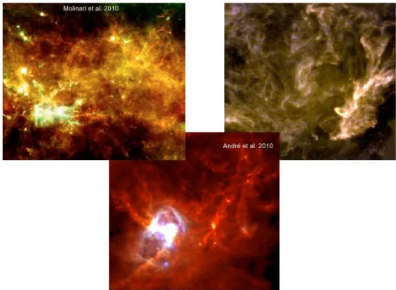
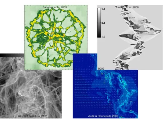
In the last years, it became more and more clear that filaments play a cru- cial role in the process of star formation. Several studies, especially the results from the HSO, have shown that cores form along filaments (Molinari et al. 2010;

André et al. 2010; Schneider et al. 2012; Palmeirim et al. 2013). The details of filamentary structure and their formation are described in Sect. 2.1.4.

In analogy to the IMF, a similar description for the mass of molecular clouds

(Williams and McKee 1997; Rosolowsky 2005) can be found, where a major

fraction of the mass is found in the larger clouds (Stark and Lee 2006). The

combination of this mass-size relation and the mass distribution of molecular

clouds explains the fractal structure of observations of these clouds (Stutzki et

al. 1998), and vice versa. The same is true for embedded high density molecular

cores, for which a distribution, a core mass function (CMF), can be given (Lada

et al. 2007; Onishi et al. 2002). The distribution of clouds and cores usually

shows a shape similar to the IMF, with a power-law tail on the high-mass end

(Stutzki and Guesten 1990; Könyves et al. 2010), but with a different spectral

index.

Fig. 2.2: Shift between IMF and CMF from Könyves et al. (2010).

This similarity of the IMF and the CMF implies that the mass of the cores directly determines the mass of the resulting stars. Also, the star formation rate (SFR), the amount of mass formed to stars in a certain time, depends directly on the clouds density (see e.g. Kennicutt 1998). However, the IMF is shifted to lower masses (Matzner and McKee 2000), which means that only a fraction of the initial cloud’s gas mass is transformed into a core and only a fraction of this core actually forms a star (see Fig. 2.2). The respective efficiencies are found to rely on the density of the cloud, thus the denser a molecular cloud is, the more of its mass will be forming stars later (e.g. Burkert and Hartmann 2013). Usually, the efficiency is quite low; Myers et al. (1986) find a value of 2 %, Evans et al.

(2009) one between 3 and 6%. The Schmidt-Kennicutt Law,

Σ

= (2.5 ± 0.7) × 10

Σ

M pc

M kpc

yr

, (2.4) however, found in Kennicutt (1998), is often used to describe the star formation rate in a galaxy.

From here on, we describe the low-mass star formation process, which is quite well known, and describe differences to high-mass star formation later.

Cores tend to collapse due to the gravity of the enclosed mass. The time-scale of this collapse, the free-fall time,

f

=

r 3 π

32 Gρ = 1.37 × 10

s

10

cm

n

year, (2.5)

2.1. ASTROPHYSICAL BACKGROUNDS 9 describes the collapse of a pressure-free, spherical cloud of density ρ, pa- rameterized to the number density of hydrogen n

. However, its kinetic energy, the presence of magnetic fields, and turbulences work against gravity and pro- vide stability for the core (see e.g. Larson 2003). This increases the collapse timescale. A core is called magnetically supercritical when its magnetic field is too low to keep the core stable, which will result in the collapse of the core. The collapsed core is then called a protostar.

During the collapse, angular momentum and magnetic field play important roles. The angular momentum that is still left in the core is usually orders of magnitudes higher than that in the later star. It can result in the formation of a binary system (Bodenheimer 1978) or will form a rotating protostellar disk surrounding the protostar (Hayashi et al. 1982; Toomre 1982). The amount of magnetic flux trapped in the initial core will also mostly drop by a factor of 10

to 10

(Nakano 1983), possibly through ambipolar diffusion, which moves the charged particles (only a small fraction of the gas) out of the neutral gas. This diffusion of the magnetic flux could be efficient enough for clump densities of n > 2 × 10

cm

(Draine 2011, p. 461). Crutcher et al. (2009) find that most cores are magnetically subcritical.

The initial hydrostatic core, or star embryo, is very small (a few AU) and has little mass (∼0.01 M ) as found by Low and Lynden-Bell (1976). However, ac- cretion from the surrounding diffuser cloud can still increase the mass of the protostar. This is called Bondi-Hoyle accretion (Hoyle and Lyttleton 1939; Bondi 1952). Most matter will first accrete onto the disk surrounding the protostar.

These disks have typical sizes of a few 100 AU (Vorobyov 2011) and lifetimes τ of several Myr with a relationship of τ ∼ 1/M (Hernández et al. 2007). The dy- namics in the disk, assuming its material is somewhat viscous, transport angular momentum outward (Lynden-Bell and Pringle 1974), which allows the material to finally fall onto the protostar and increase its mass.

But not all matter in the disk is funneled onto the protostar. Magnetic winds drive great parts of the disk mass toward the center, but then create jets that are directed away from the protostar, perpendicular to the disk. These jets guide ionized and molecular gas back into the ISM, which is seen as bipolar outflows in observations (e.g. Edwards et al. 1993). One example is shown in Fig. 2.3.

At a mass of about 0.2 M , deuterium burning sets in, which stabilizes the star and keeps it from further collapsing. It usually accretes more mass, up to a certain radius (about 4 R for a star of 1 M , see Stahler et al. 1980), when the surrounding mass reservoir is used up and accretion does not play a role anymore. From here on, the low-mass star follows the usual evolution.

There are certain differences in the evolution of high-mass stars of masses

larger than 8 M , although many details are not yet understood. See also

Beuther et al. (2007) for a review. High-mass stars often form in clusters,

where several cores are embedded in a molecular cloud (Klessen and Burk-

ert 2001), mostly along filaments (André et al. 2010; Molinari et al. 2010, see

Fig. 2.3: Protostellar jet observed at 2.12 µm with the Infrared Astronomical Satellite (IRAS). H

emission of the object HH212 as described in Zinnecker et al. (1997).

also Sect. 2.1.4). In these clusters, protostars form from accretion and mergers, which leads to growth (e.g. Bonnell et al. 2003). The final mass is essentially de- termined by the mass of the formation environment and not by the single cores mass. The most massive stars will form in the center of the cluster. As larger cores accrete the most mass and eat away the molecular clouds in their vicinity, the model is also called competitive accretion model.

In contrast, in the monolithic collapse model, single high mass stars of up to 140 M can form from turbulent cores (Kuiper et al. 2010). The mass of the initial clump limits the stars final mass. This model is basically a scaled-up low-mass star formation model, where a disk forms early and mass outflows transport radiation away and allow further accretion of mass.

High mass stars form from cores with masses above the Jeans mass, which Evans (e.g. 1999) stated, can have densities of more than 10

cm

and temper- atures of more than 100 K. They are so massive that they already start nuclear fusion during the accretion process, which leads to feedback effects. This feed- back was first thought to stop accretion so that stars could not become more massive than a few tens of M (Wolfire and Cassinelli 1987). However, the for- mation of jets that transport radiation to the outside should increase accretion and allow for higher masses (Banerjee and Pudritz 2007).

The radiation of high-mass stars ionizes the surrounding molecular gas and creates H II regions

. Depending on size and density, these regions are called ultra compact H II regions (UCHIIs), with densities of >10

cm

and sizes of <0.1 pc, or hyper compact H II regions (HCHIIs), that can have densities

>10

cm

and sizes of <0.05 pc, according to Kurtz (2005) and Hoare et al.

(2007). This radiation can disrupt GMCs and return their matter back to the dif-

1

This is the spectroscopic notation of ionized hydrogen.

2.1. ASTROPHYSICAL BACKGROUNDS 11 fuse ISM (McKee and Ostriker 2007). From there, the cycle of molecular cloud formation and star formation can begin anew (see also Fig. 2.1).

2.1.2 Interstellar medium

As already mentioned in Sect. 2.1.1, our Galaxy does not only contain stars, but also a huge amount of gas and dust (which account for ∼ 10 − 15% of the total mass of the Galaxy) that fills the space in-between them. The fraction of mass found in gas form is usually much higher in young galaxies (Popping et al.

2013), as only a fraction of the mass could be transformed into stars, yet. We call this phase the ISM, which includes all material that is gravitationally bound to galaxies, except for the stars (and dark matter). In contrast, the intergalactic medium (IGM) identifies the phase between galaxies.

The ISM is composed of several parts (see Table 2.1, values taken from Fer- rière 2001; Draine 2011): molecular clouds, the neutral gas, ionized gas, and dust. The ISM gas mainly consists of hydrogen and helium that have been cre- ated shortly after the big bang. All higher elements have been formed by nucle- osynthesis in stars.

(1) (2) (3) (4)

Phase Temperature Density Volume fraction

[K] [cm

] [%]

Molecular gas 10-20 10

-10

1

CNM 50-100 20-50 1-5

WNM 6000 0.5 10-20

WIM 6000 0.5 20-50

HIM 10

10

30-70

Table 2.1: Different phases of the ISM and their properties.

Molecular gas is the coldest and densest part of the ISM and only takes up a small fraction of its volume (see Table 2.1 for detailed values). However, the hydrogen in the molecular gas still contains 18% of the total hydrogen mass of the ISM, due to its high density. The total molecular hydrogen mass in the Milky Way is found to be 8.4 × 10

M . This phase is the most important one in the context of this work and the formation of molecular clouds from the neutral gas is described in more detail in Sect. 2.1.3.

The neutral atomic part of the ISM consists of neutral hydrogen and is warmer and diffuser than the molecular clouds. It consists of two phases of dif- ferent temperature and density that can coexist in pressure equilibrium, due to the bistable nature of the neutral gas. This model is described by Field et al.

(1969) and refined by Wolfire et al. (1995). The phases are called the cold neu-

tral medium (CNM), which has medium temperature and density, and the warm

neutral medium (WNM), which has higher temperature and lower density. The CNM and WNM account for about a fifth of the volume of the ISM. The total mass of the H I is 2.9 × 10

M , which is equivalent to 60% of the total hydro- gen mass in the ISM gas. Parts of the WNM are ionized by X-rays and cosmic rays and form the warm ionized medium (WIM) that has the same density and temperature structure as the WNM.

Shock fronts in the WNM induce the transition to the CNM. Usually, these shock fronts are unstable and thermally fragmented (Koyama and Inutsuka 2002). Therefore, also the CNM is very fragmented, as seen in several simu- lations (e.g. Audit and Hennebelle 2005; Heitsch et al. 2005).

McKee and Ostriker (1977) extended the two-phase model by a third compo- nent, the hot ionized medium (HIM), which is heated by supernovae and reaches very high temperatures and low densities (Gent et al. 2013). It fills the remain- ing space of the ISM. The warm and hot ionized hydrogen contributes 23%

(1.1 × 10

M ) of the total hydrogen mass, contained in the ISM of the Galaxy.

Finally, dust plays an important role in the ISM. It was found that dust emis- sion correlates quite well with the emission from molecular clouds (Bohlin 1975).

Dust consists of grains that are mainly composed of graphites, silicates, or water ice (Ferrarotti and Gail 2006; Voshchinnikov and Henning 2010; Sirono 2013).

Mathis et al. (1977) could reconstruct the size distributions of these grains from dust extinction curves. They found a power-law for the distribution of radius a,

N (a)da ∝ a

da, (2.6)

in the range of 0.005-1 µm (a newer distribution can be found in Casuso and Beckman 2010). On the low-end of the size scale, polycyclic aromatic hydro- carbons (PAHs) (Leger and Puget 1984; Lebouteiller et al. 2011) are the bridge between dust grains and organic macro-molecules. Dust grains can form in the cool atmosphere of red giants and planetary nebulae (Woolf and Ney 1969;

Salpeter 1976), as well as in the ISM itself (Dwek and Scalo 1980).

There is much more gas than dust found in the ISM. The typical gas-to-dust mass ratio is on the order of 100, but can be even higher in some regions (Frisch and Slavin 2003; Parkin et al. 2012). The temperature of the interstellar dust is found to be between 10 and 30 K in most regions (Planck Collaboration et al.

2011; Galametz et al. 2012).

It is important to note that dust aids in the creation of molecules. H

molecules have to mainly form on grain surfaces (Hollenbach and Salpeter 1971;

Charnley and Rodgers 2009) and dust helps to shield the molecules from photo-

dissociation by UV radiation (Shull and Beckwith 1982). It can also be destroyed

by shocks and release contained atoms and molecules to the gas phase (Seab

1987; Van Loo et al. 2013). SiO is a typical tracer for these shocks, because it

2.1. ASTROPHYSICAL BACKGROUNDS 13 is released from the destroyed dust grains (Schilke et al. 1997). Therefore, dust acts as an important reservoir for many elements, especially Mg, Si, Fe, but also a good fraction of carbon (80%) and oxygen (15%) are contained in dust (Kim et al. 1994; Dwek et al. 1997). It also plays a crucial role in heating and cooling mechanisms of molecular clouds, as described by Watson (1972), Burke and Hollenbach (1983), or Xilouris et al. (2012).

Therefore, dust emission and absorption observations can be interesting tools to gather information on molecular clouds and their properties. We will utilize this later in this work.

2.1.3 Molecular cloud formation

As discussed in Sect. 2.1.1, stars form in molecular clouds that are part of the ISM. We will now describe how these clouds form from the diffuse atomic gas, as introduced in Sect. 2.1.2. Observationally, carbon monoxide is often used to trace molecular clouds, as cold molecular hydrogen is hard to detect, due to its missing permanent electric dipole moment (see Sect. 2.2.4, where the physics of molecular emission lines is explained in more detail). CO in contrast, is easy to detect and sufficiently well mixed with hydrogen to use it as a proxy for molecular cloud observations.

Williams et al. (1995) discovered an anti-correlation between CO and H I emission in the Rosette nebula. They concluded that atomic and molecular clouds are related but mutually exclusive. The atomic hydrogen forms a halo around the molecular clouds and fills the inter-cloud medium. However, Li and Goldsmith (2003) also find H I in molecular clouds.

As molecular clouds show a large level of turbulence, we can assume this energy to originate from the initial atomic clouds. Continuous accretion of molec- ular gas from the surrounding H I probably drives turbulence (Klessen and Hen- nebelle 2010; Goldbaum et al. 2011).

For nearly ten years, theoreticians have now produced models of the molec- ular cloud formation. One class of models describes the interaction of collid- ing flows (also called converging flows). There have been calculations by differ- ent groups, for example, published in Audit and Hennebelle (2005); Vázquez- Semadeni et al. (2007); Hennebelle et al. (2008); Heitsch et al. (2008); Banerjee et al. (2009).

These models base on two flows of warm atomic hydrogen gas that stream toward each other. The principle setup is depicted in Fig. 2.4. The turbulences at the impact region let the WNM collapse into CNM clouds in which molecular clouds can associate.

Of course, this setup is very simplistic and is most probably not found in real-

ity in this way. The simulation of specific star-forming regions is nearly impossible

Fig. 2.4: Colliding flows model from Vázquez-Semadeni et al. (2007).

at the moment, as exact starting values for the models have to be found. Still, modeling has made important progress in the last years and can explain molec- ular cloud formation, at least in principle.

The structure of the molecular clouds is usually very complex and follows the structure of the CNM. The clumps are bounded by the WNM, which provides a confining pressure.

It is possible that star formation already sets in, while the cloud is still ac- creting (Vázquez-Semadeni et al. 2007). Different tools have been developed to distinguish between quiescent and star-forming clouds. One possibility is the use of PDFs of the H

column density (see Kainulainen et al. 2009) that we also use in our analysis later. This method creates a histogram of the column density data and analyzes the resulting shape. Quiescent regions are found to have a log-normal distribution, while star-forming regions show a power-law excess at the high-mass tail of the function (Klessen 2000; Schneider et al. 2012).

Another technique is the calculation of the ∆-variance, developed by Stutzki et al. (1998); Ossenkopf et al. (2008b,a). It is a measure for the characteristic scale in a dataset. It can measure typical widths of filaments but can also provide information on the form of turbulence in a cloud and therefore star formation activity (Rowles and Froebrich 2011).

Most models of molecular clouds have in common that parts of the clouds

arrange in filamentary structures. This is an important result, as it is known from

2.1. ASTROPHYSICAL BACKGROUNDS 15 observations that star-forming cores are found along these filaments. Therefore, we will now discuss these structures and their development in more detail.

2.1.4 Filamentary structure

Fig. 2.5: Examples of filaments in observations. Left: Molinari et al. (2010), showing infrared dark clouds (IRDCs) in the Galactic plane at 59

Galactic longitude Herschel infrared Galactic Plane Survey (Hi-GAL) map. Center: Aquila field from the Herschel Gould Belt Survey as described in André et al. (2010). Right: Polaris field from the same project.

As mentioned above, filaments are pervasive in recent observations of molecular lines and dust emission (André et al. 2010; Molinari et al. 2010;

Schneider et al. 2010). But also earlier observations show these objects (e.g.

Dutrey et al. 1991). Here, filaments are defined as coherent, elongated struc- tures that are seen in emission or absorption. Figure 2.5 shows a few examples of filaments observed with the HSO. The typical filament in these observations has a width of 0.1 pc, as measured by Arzoumanian et al. (2011), but the defi- nition of what exactly is called a filament can change. These values stem from dust total power maps that average out possible sub-structure. Additional veloc- ity information and high spatial resolution show that large filamentary clouds can often be broken down into smaller filaments (e.g. Hacar et al. 2013).

Again, as mentioned above, filaments are also found recurrently in the mod-

Fig. 2.6: Examples of filaments in simulations. Left: Model from Glover and Mac Low (2007), three-dimensional hydrodynamics with self-gravitation and non-equilibrium chemistry. Center left: 3D colliding flows model using weakly magnetized magneto- hydrodynamics (MHD) simulations (Banerjee et al. 2009). Center right: 2D purely hy- drodynamical model from Audit and Hennebelle (2005). Right: Pure hydrodynamics 3D model, as presented in Heitsch et al. (2006).

els of molecular cloud formation: Padoan et al. (2001); Audit and Hennebelle (2005); Heitsch et al. (2006); Glover and Mac Low (2007); Hennebelle et al.

(2008); Nakamura and Li (2008); Inoue and Totani (2009); Vázquez-Semadeni et al. (2011); this is a non-exhaustive list of works. There are three fundamental processes that can play a role in filament formation: gravity, turbulences, and magnetic fields. Each of the mentioned simulations takes one or more of these into account.

Models based on pure gravity can create filaments from fragmentation of sheets of gas. Self-gravity enhances anisotropies in the mass distribution, thus, somewhat elongated clouds will soon collapse to filaments (Myers 2009), which will further break down and form cores along them (Ostriker 1964; Fiege and Pu- dritz 2000). In MHD turbulence models, the filamentary structure can be induced by turbulence (Padoan et al. 2001). Including gravity, these initial structures can be selected and further enhanced by gravity, creating cores (Hennebelle and Chabrier 2008). Magnetic fields can add stability to filaments.

It is yet unclear which specific setup of turbulence, MHD, and gravity is most

realistic. Until now, it is not possible to actually distinguish between different

2.1. ASTROPHYSICAL BACKGROUNDS 17 models using observations. More advances in models and observations are needed for this purpose.

2.1.5 Structure of the Milky Way

Making statements about the structure of the Milky Way is inherently compli- cated, since the Solar system is located inside the Galaxy. We have to try and reproduce the distribution of matter by observing the velocity structure of the visible radiation. Via the relative velocities of stars and clouds it is possible to create a model of the Galaxy. A comparison with extragalactic observations of similar galaxies can help to verify this model.

Fig. 2.7: Artists view of the Galaxy. The assumed location of W43, the object of interest in this work, is marked by the black star. Credits: R. Hurt, Caltech.

Basically, it has been known for decades that our Galaxy is a spiral galaxy. It

was discovered later that, to be more precise, it has to be considered a barred

spiral galaxy (Chen et al. 1996). Many single observations of different parts of

the Galaxy and at different wavelengths have been carried out to determine the

number, shape and angle of the spiral arms. Meta-studies of dozens of studies

from the years 1980 to 2005 are given in Vallée (1995, 2002, 2005) and in Vallée

(2008) a simple model of our Galaxy is designed. Figure 2.7 shows a face-on

view of the Milky Way, created by an artist, according to the models.

Our Galaxy consists of a flat, nearly circular disk that contains spiral arms and surrounds the Galactic center. Beside the stars, it contains large amounts of dust, atomic, and molecular gas (Levine et al. 2006). A bulge surrounds the inner few kpc spherically and extends above and below the disk. Sometimes, it is rather described as an elliptical pseudo-bulge. Disk and bulge are again embedded into the spherical Galactic halo that contains mostly old stars, but hardly any molecular gas or dust. The size of the halo is roughly defined by the distances of our neighboring dwarf galaxies, the Large and Small Magellanic Clouds (Connors et al. 2006).

The center of the Galaxy, about 8.5 kpc remote from the Sun, contains a super-massive black hole that is found to have a mass of ∼3 − 4.5 × 10

M

(Genzel et al. 2000; Ghez et al. 2008). The diameter of the Galaxy is usually given as ∼30 kpc, in which it contains a total mass of about 10

M , the height of the disk is approximately 0.3 kpc (Rix and Bovy 2013).

It is debated (see Nishiyama et al. 2005) whether the center of the Galaxy contains not only a single bar, but two separate bars, the regular Galactic bar and the elongated bar. The assumed lengths of the bars are typically 3 kpc (Rodríguez-Fernández and Combes 2008). Scientists usually agree that four Galactic spiral arms exist (Churchwell et al. 2009), which connect to the tips of the bars. One set of arms, the Perseus and the Scutum-Centaurus arm, are brighter and wider, while the other set, the Norma or Outer arm and the Carina- Sagittarius arm, are fainter and smaller. These arms wind around the Galactic center in logarithmic outward spirals. Additionally, there are two weak arms that are called the near and the far 3-kpc arm that connect both ends of the elongated bar with each other (Rodríguez-Fernández 2011). Finally, several spurs, or arm fragments, can be found in-between the main spiral arms, one of which is the Orion-Cygnus spur that contains the Sun.

There is a fundamental difference between the spiral arms region and the bars. Stars and matter in both regions orbit the Galactic center but their orbits differ. Orbits in the spiral arms are circular (Lin and Shu 1964; Lynden-Bell and Kalnajs 1972; Gómez et al. 2013), whereas elliptical orbits are found in the bars (e.g. Binney 1982; Sanders et al. 1983; Pichardo et al. 2004). The spiral arms are thought to form due to waves of increased density that move outward from the Galactic center. In this model the inter-arm medium would move in and out of the arms, where it is compressed. This increased density would initiate the formation of molecular gas and finally star-formation would set in (e.g. Moore et al. 2012; Eden et al. 2013).

Although stars and gas at all Galactic radii rotate around the center, the ro-

tation velocity changes with the radius. This rotation curve is an important tool

for the calculation of distances in the Milky Way and is therefore strongly de-

bated. Rotation speed in the central part of the Galaxy roughly rises linearly

with the radius. Outside the bar, the rotation curve is mostly flat, which means

that rotation does not depend on the distance toward the Galactic center (see

e.g. Clemens 1985; Reid et al. 2009). These observed velocities contradict the

2.2. SUBMM/MM-ASTRONOMY 19 amount of mass that can actually be detected. According to the observed dis- tribution of mass, the rotation curve should decrease for larger radii (Rubin et al. 1980, describe this phenomenon in extragalactic galaxies). The hypothesis of dark matter tries to explain this lack of mass by postulating the existence of hitherto undetectable mass. This question touches some of the fundamentals of physics and is still not answered to date.

The presumed location of the W43 star-forming region, the region of interest in this thesis, is shown by the black star in Fig. 2.7.

2.1.6 The W43 star-forming region

The region at 30

Galactic longitude in the Galactic plane was first identified by Westerhout (1958), who listed it in his catalog as W43. About 10 years ago, this object was identified as one of the most active star-forming regions in the Galaxy (Motte et al. 2003). It was shown to be heated by a cluster of Wolf-Rayet and OB stars (Lester et al. 1985; Blum et al. 1999) and Motte et al. were the first to consider it as a Galactic mini-starburst region.

The name W43 was initially used for the single cloud (G030.8+0.02) that is known today as W43-Main. Nguyen Luong et al. (2011) characterized the complex by analyzing Very Large Array (VLA) H I emission (Stil et al. 2006) and the

CO (1–0) (Dame et al. 2001) and

CO (1–0) (Jackson et al. 2006) Galactic plane surveys. They concluded that W43-Main and G29.96-0.02 (also called W43-South) should be considered as a single giant connected complex.

From the position in the Galactic plane and its radial velocity, Nguyen Luong et al. (2011) concluded that W43 is located at the junction point of the Galactic long bar and the Scutum spiral arm at 6 kpc relative to the Sun (see black marker in Fig. 2.7). The kinematic distance ambiguity, arising from the Galactic rotation curve, gives relative distances for W43 of ∼6 and ∼8.5 kpc for the near and the far kinematic distance, respectively. Although there have been other distances adopted by other authors (e.g. Pandian et al. 2008), most publications (Pratap et al. 1999; Anderson and Bania 2009; Russeil et al. 2011) favor the near kinematic distance. In Sect. 4.4 we will confirm this distance determination.

This position in the Galaxy makes W43 a very interesting object for studying

the formation of molecular clouds. Despite its distance, it is possible to analyze

the details of this cloud, due to its large spatial scale of ∼150 pc and the large

amount of gas at high density (see Nguyen Luong et al. 2011). As discussed

above, this junction point in the Galactic plane is an ideal laboratory to study the

circumstances of molecular cloud formation.

Fig. 2.8: Transmission of the atmosphere. Credits of image: NASA/Infrared Processing and Analysis Center (IPAC).

2.2 Submm/mm-Astronomy

The spectral window of a few mm (about 100–350 GHz) has become one of the most used in radio astronomy in the last decades. Higher frequencies in the sub-millimeter regime (up to a few THz) are more complicated to observe, but improved telescopes and receivers have begun to make this part of the spec- trum available to astronomy. These frequency ranges are especially important for research of the ISM. Many molecular emission line transitions fall in these spectral windows. In contrast to lower radio frequencies, the atmosphere is not completely transparent at these frequencies (cf. Fig. 2.8). The higher the fre- quency, the more radiation is absorbed, mostly by water vapor. Due to this char- acteristic of the atmosphere, submm/mm telescopes need to be located as high as possible at places as dry as possible. A very good location is the Atacama desert in Chile (ALMA, APEX, NANTEN2). To further reduce the atmospheric absorption, telescopes are also mounted on planes (Stratospheric Observatory For Infrared Astronomy (SOFIA)), balloons (Stratospheric Terahertz Observatory (STO)), and of course satellites (HSO). Unfortunately, the better the conditions, the more costly and complicated the operations are.

We use a variety of telescopes in our work that operate at these frequencies.

We will hence give a short introduction into the functionality of radio telescopes.

2.2. SUBMM/MM-ASTRONOMY 21 2.2.1 Radio telescopes

For an exhaustive description of the technical background in this and the next subsections see, for example, Wilson et al. (2009). Single-dish antennas, the most common type of telescopes used in radio astronomy, usually consist of a circularly symmetric paraboloid dish (or mirror), although sometimes dipole antennas are used for very low frequencies (e.g. in the Low-Frequency Array (LOFAR) and in future in the Square Kilometre Array (SKA)). The incoming ra- diation from the sky is reflected to a secondary mirror, which focuses the signal into the optics of the telescope and finally into the receiver.

The beam pattern of a telescope is the Fourier transform of the shape of the aperture (in optical astronomy, the aperture is just a disk and the beam pattern therefore the square of the Bessel function). In radio astronomy, this pattern is re- fraction limited and depends on the exact geometry of the telescope. The beam pattern of a parabolic telescope is basically a Gauss function, convolved with the disk of the main mirror, which leads to a beam pattern with a strong Gaus- sian maximum in boresight and smaller off-axis maxima, so-called side lobes, induced by the cutoff of the Gaussian at the edges. Additionally, the shadowing of the secondary mirror, its suspension legs in the main beam, and the reflection of the beam onto the secondary mirror, add further changes to the final beam pattern. It can only be numerically determined, but the central maximum usually still remains mostly Gaussian.

The distribution of intensities on the sky is convolved with this beam pattern and the integral is then fed into the receiver. This means that information of more than one point on the sky goes into the signal, which can be a problem, when observing extended emission. The weighting is determined by the beam pattern. Side lobes (typically on the order of 10 to 20 dB) can be reduced by only illuminating the inner part of the main dish, however, this tapering reduces sensitivity and resolution of the telescope.

The half power beam width (HPBW) of a radio telescope depends on the details of the beam pattern and the tapering, but can be fitted by the formula

∆θ

= (1.02 + 0.0135 T

) λ

D , (2.7)

from Goldsmith (1996), with the wavelength λ, the diameter of the primary mirror D, and the edge taper T

in dB. Two points on the sky can still be distinguished if they are separated by this angle. This means that the resolution increases with the telescope size and with the frequency. To regain the full information of the distribution of emission on the sky, filtered by the beam, the spatial sampling of observations has to be below λ/2D (Nyquist sampling).

Unfortunately, higher frequencies require a higher accuracy of the telescope

surface so that it still acts as a mirror. The root mean square (rms) deviation

of the surface has to be on the order of λ/20. Therefore, in order to observe the same level of detail, we need larger telescopes, but with less accuracy of the surface, at low frequencies and smaller dishes with high surface accuracy at high frequencies.

For example, the Effelsberg telescope operates at frequencies between 0.4 and 86 GHz, has a diameter of 100 m and a surface accuracy of 0.5 mm, which is a great achievement for this antenna size. In contrast, the Cerro Chajnantor At- acama Telescope (CCAT) will use frequencies between 150 GHz and ∼1.5 THz.

It will will have a diameter of 25 m and a surface accuracy of less than 10 µm, an extremely demanding technical requirement.

2.2.2 Receivers used in radio astronomy

The radiation from the sky, that has been focused by the antenna, needs to be amplified, filtered by direction, frequency, and polarization, and converted to an electrical signal to be usable. These different steps are done by receivers that convert the electromagnetic radiation into electrical voltage, amplify it, and nowadays mostly convert it to digital information.

Different receiver designs serve different purposes in radio astronomy. For a high sensitivity of continuum observations over a large bandwidth, bolometers are often used. They measure the temperature change of an absorber, induced by the absorption of photons. This temperature change can be used to determine the energy of the absorbed radiation. Bolometers do not preserve the spectral information, phase, or polarization of the detected photons. Bolometers are best used for total power measurements, where they can be extremely sensitive. They can be combined with spectrometers or polarizing devices in front of them to regain this information but loose sensitivity that way. These measurements are more complicated and the resolution is limited with these devices.

Heterodyne receivers are widely-used for high resolution spectroscopic ob- servation. Their advantage over bolometers is that they preserve frequency in- formation through the filtering process. These receivers amplify and then con- vert the signal from the sky to a lower frequency, by mixing it with a pure sine- wave from a local oscillator (LO). This synthesizer signal is shifted by a few per- cent from the sky signal (usually a few GHz). The resulting mixed signal has a lower frequency, that still contains all the astronomical information and can then be filtered and further amplified. Superconductor-insulator-superconductor (SIS) junctions are nowadays often used as mixers, as they provide a good spectral resolution and large bandwidth (several GHz). However, from frequencies on the order of THz, SIS mixers suffer from losses. At this range hot electron bolometer (HEB) mixers have the advantage of a lower noise level, but only have a limited bandwidth of a few MHz.

Heterodyne receivers have the advantage of mostly preventing feedback ef-

fects during the amplification of the signal. Without the frequency conversion

2.2. SUBMM/MM-ASTRONOMY 23 (homodyne receivers), it is possible that amplified signal leaks back into the ini- tial signal. In addition, these receivers are easier to tune to the desired frequency by changing the LO signal. Finally, it is more complicated to build amplifiers that work at very high frequencies. This can be circumvented by amplifying the lower frequency in heterodyne receivers.

The part of the receiver that works at sky frequency is usually called frontend, while the part that works at the down-converted frequency is called a backend.

Frontends can consist of one (single-pixel receivers) or several (array receivers) mixers. Arrays can observe several positions on the sky simultaneously, which is efficient if an observation includes many points or complete maps.

Spectrometers are backends that resolve the spectral information of the sig- nal. There are several ways of doing so. One possibility are acusto-optical spec- trometers (AOSs), where the signal is converted to an acoustic signal and fed into a special crystal (Bragg-cell), whose refraction behavior is changed. A laser, pointed at the cell, is deflected depending on the frequency of the incoming sig- nal and then reaches a matrix of charge-coupled devices (CCDs) that pick up the laser at different positions. Thus, the Bragg-cell acts as a natural Fourier trans- formation of the input signal. Fourier-transform spectrometers (FTSs) digitize the time dependent signal and transform it to a spectrum using raw computing power. These spectrometers are becoming the new standard, since computers have become fast enough to provide enough bandwidth and resolution.

For spectrometers, the sensitivity ∆T that can be reached depends on the systems noise temperature T

, the desired spectral resolution ∆ν , and the ob- serving time t:

∆T

T

∝ 1

√

∆ν t . (2.8)

The needed observing time can be quite large (sometimes hours or more), there- fore, the receiver needs to be as stable as possible, but will rarely reach a stability of more than a few minutes. Both, the total gain and differences along the spec- tral axis will change over time. Therefore, observations often need to be split up into shorter observations, with gain calibrations conducted in-between.

In addition, the instability of the atmosphere has to be taken into account. It

will usually change on the order of minutes and can be dealt with, by observing

not only the astronomical target (on-position), but also a nearby blank position

on the sky (off-position). The difference of both spectra is therefore the desired

signal, adjusted for atmospheric and receiver effects. This position switching

method is used when observing single positions on the sky. For large objects,

the on-the-fly (OTF) method is more efficient. Here, several positions are con-

secutively observed while the telescopes slews across the sky and share one

common off-position. This is the observational technique which is most often

used in this work.