Universität Konstanz Sommersemester 2013 Fachbereich Mathematik und Statistik

Universität Konstanz Sommersemester 2013 Fachbereich Mathematik und Statistik

Prof. Dr. Stefan Volkwein

Roberta Mancini, Stefan Trenz, Carmen Gräßle, Marco Menner, Kevin Sieg

Optimierung

http://www.math.uni-konstanz.de/numerik/personen/volkwein/teaching/

Program 2

Submission by E-Mail: 2013/06/17, 10:00 h

Note: Stick to the given function and parameter definitions as described below!

You should not modify them in name or concerning the input and output arguments.

Implementation of the Projected Gradient Method.

Part 1: Generate a file projection.m and implement the function function [px] = projection(x, a, b)

with the current point x ∈ R ⁿ , lower bound a ∈ R ⁿ and upper bound b ∈ R ⁿ as input arguments. The function returns the (pointwise) projected point px ∈ R ⁿ according to the projection

P : R ⁿ → Ω := {x ∈ R ⁿ | ∀i = 1, ..., n : a _i ≤ x _i ≤ b _i }.

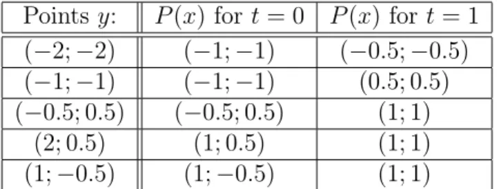
Test your function for the rectangular 2-D domain defined by the lower bound (lower left corner) a = (−1; −1) and the upper bound (upper right corner) b = (1; 1): compute the projection P (x) of points x = y + td ∈ R ² with y ∈ R ² as given in the table below, direction d = (1.5; 1.5) ∈ R ² , step sizes t = 0 and t = 1. For validation compare your results to the projections given in the table:

Points y: P (x) for t = 0 P (x) for t = 1 (−2; −2) (−1; −1) (−0.5; −0.5) (−1; −1) (−1; −1) (0.5; 0.5) (−0.5; 0.5) (−0.5; 0.5) (1; 1)

(2; 0.5) (1; 0.5) (1; 1)

(1; −0.5) (1; −0.5) (1; 1)

Table 1: Testing points and their projections with respect to t

Part 2: Write a function

function [t] = modarmijo(fhandle, x, d, t0, alpha, beta, a, b)

for the Armijo step size strategy with the modified termination condition f(x(λ)) − f(x) ≤ − α

λ ||x − x(λ)|| ²

with current point x, descent direction d, initial step size t0, alpha and beta for the Armijo rule and a and b for the projection rule.

Part 3: Implement the gradient projection algorithm with direction d k := − _k∇f ^{∇f (x} _(x

⁾

k

)k . Generate a file gradproj.m for the function

function [X] = gradproj(fhandle, x0, epsilon, nmax, t0, alpha, beta, a, b) with initial point x0, parameter epsilon for the termination condition k∇f(x k )k < and the additional termination condition kx − x(1)k < , nmax for the maximal number of iteration steps, parameters t0, alpha and beta for the Armijo rule and a and b for the projection rule. Modify therefore the gradient method gradmethod.m.

The program should return a matrix X = [x0; x1; x2; ...] containing the whole iter- ations.

Part 4: Call the function gradproj from a main file main.m to test your program for the Rosenbrock function

function [f,g] = rosenbrock(x)

with input argument x ∈ R ² and output arguments the corresponding function value f

∈ R and gradient g ∈ R ² . Use the following parameters and write your observations in the report:

epsilon=1.0e-2, N=1.5e+3, t0=1, alpha=1.0e-2, beta=0.5 and 1. x0=[1;-0.5], a=[-1;-1] and b=[2;2]

2. x0=[-1;-0.5], a=[-2;-2] and b=[2;0]

3. x0=[-2;2], a=[-2;-2] and b=[2;2]

Visualize your results by suitable plots!