What Doesn’t Kill You Makes You Poorer

Policy Research Working Paper 7121

What Doesn’t Kill You Makes You Poorer

Adult Wages and the Early-Life Disease Environment in India

Nicholas Lawson Dean Spears

Water Global Practice Group November 2014

WPS7121

Public Disclosure Authorized Public Disclosure Authorized Public Disclosure Authorized Public Disclosure Authorized

Abstract

The Policy Research Working Paper Series disseminates the findings of work in progress to encourage the exchange of ideas about development issues. An objective of the series is to get the findings out quickly, even if the presentations are less than fully polished. The papers carry the names of the authors and should be cited accordingly. The findings, interpretations, and conclusions expressed in this paper are entirely those of the authors. They do not necessarily represent the views of the International Bank for Reconstruction and Development/World Bank and its affiliated organizations, or those of the Executive Directors of the World Bank or the governments they represent.

Policy Research Working Paper 7121

This paper is a product of the Water Global Practice Group. It is part of a larger effort by the World Bank to provide open access to its research and make a contribution to development policy discussions around the world. Policy Research Working Papers are also posted on the Web at http://econ.worldbank.org. The authors may be contacted at nicholas.

lawson@univ-amu.fr.

A growing literature documents links between early-life health and human capital, and between human capital and adult wages. Although most of this literature has focused on developed countries, economists have hypothesized that effects of early-life health on adult economic out- comes could be even greater in developing countries. This paper asks whether the early-life disease environment in India influences adult economic wages. The paper uses two measures of early-life disease environment to investigate this question: infant mortality rates and open defecation.

A district-level differences-in-differences strategy is used to show that men born in district-years with lower infant mor- tality and better sanitation earned plausibly higher wages

in their 20s and 30s. The effect estimates are applied to

calculate the fiscal and welfare consequences of the dis-

ease environment, which are considerable. In particular,

eliminating open defecation would increase tax revenue

by enough to offset completely a cost to the government

of over \$400 per household that stops defecating in the

open. A fiscally neutral elimination of open defecation in

India would increase the net present value of lifetime wages

by more than \$1,800 for an average male worker born

today. These large economic benefits ignore any other ben-

efits of improved health or reduced mortality. The result

suggests that the disease environment could have impor-

tant effects on developing-country economic outcomes.

What Doesn’t Kill You Makes You Poorer:

Adult Wages and the Early-Life Disease Environment in India

Nicholas Lawson ^∗

Aix-Marseille University (Aix-Marseille School of Economics), CNRS & EHESS

Dean Spears

Centre for Development Economics, Delhi School of Economics

JEL Codes: I15, J24, O15

Keywords: sanitation, disease environment, wages, India

∗

nicholas.lawson@univ-amu.fr. We would like to thank Diane Coffey, Aashish Gupta, Habiba Djebbari,

the participants of the International Seminar on Food Security in India at the University of Allahabad, the

WASH 2014 Conference in Brisbane, and a seminar at the World Bank Water and Sanitation Program in

Delhi. Any errors or omissions are the responsibility of the authors.

1 Introduction

A growing literature documents that workers exposed to a better disease environment in early life earn higher wages as adults. Although this literature has focused on developed countries, economists have hypothesized that this effect of early-life disease externalities could be importantly larger in developing countries, where disease insults are worse and more varied (Currie and Vogl, 2013; Spears, 2012b). If early-life disease indeed importantly limits human capital in developing countries, wages could be a mechanism through which health has important effects on developing economies and, because of income and consumption tax revenue, on the government’s budget. It is therefore important to understand and quantify effects of the disease environment on subsequent wages in developing countries.

Our paper examines the impact of the early-life disease environment on adult wages in India. We match male workers in nationally representative survey data on wages in the 2000s to district-level census data from the 1970s and 1980s on two important measures of disease environment: infant mortality and santitation coverage. Our results suggest that being born in a district-year with widespread open defecation or a high infant mortality rate significantly reduces earnings decades later. Because infant mortality and open defecation remain significant threats to health in India and other developing countries, these estimates are of continuing economic and policy importance.

Poor sanitation, and infectious disease more generally, are well-known to have negative

externalities on neighbors (Galiani, Gertler, and Schargrodsky, 2005; Geruso and Spears,

2014). We show that the disease environment also has fiscal externalities: we estimate

considerable effects on government tax revenues of reductions in income and consumption

due to early-life disease. In particular, our baseline results indicate that reducing open

defecation would increase tax revenue by enough to completely offset a cost of up to $462

per household that stops defecating in the open. We find that a fiscally neutral elimination

of open defecation in India would increase the net present value of lifetime after-tax wages by

more than $1800 for an average male worker born today. Therefore, the main contribution of

this paper is to show that partial causal effects already understood to exist in the literature

– the effect of the epidemiological environment on early-life health, of early-life health on

adult human capital, and of adult productivity on wages – can add up to quantitatively important overall economic and fiscal effects in the context of a developing country with a large burden of disease externalities.

The remainder of this introductory section provides a brief overview of related literature and the Indian context. Section 2 details our empirical strategy. Section 3 presents our empirical results, linking early-life disease to adult earnings. Section 4 presents computations of effects on government revenues and a simple measure of welfare. Section 5 concludes.

1.1 Early-Life Human Capital Formation and Adult Wages

An active literature in economics documents that healthier babies are more likely to become healthier and more productive children and adults (Currie, 2009). Early-life health matters because the first few years are a critical developmental period; children who have better health and net nutrition in early life are more likely to reach their physical growth potentials and are more likely to reach their cognitive potentials (Case and Paxson, 2008). Indeed, much of this literature, unable to match adult wages to early-life conditions, has used adult height as a proxy for early-life health (e.g. Vogl, 2014). Most of this literature has focused on developed countries. However, the impact of early-life disease externalities in developing countries may be an even more important part of labor market outcomes than in developed countries, relative to heterogeneity in genetic potentials: disease conditions are worse, care and remediation may be less available, and heterogeneity in health insults is likely to be larger than in developed countries.

Economists have linked various measures in the chain from early-life human capital ac- cumulation to its long-run consequences: childhood and adult height, childhood and adult cognitive achievement, and adult wages. For example, Bozzoli, Deaton, and Quintana- Domeque (2009) show that people are shorter in countries with higher infant mortality;

Alderman, Hoogeveen, and Rossi (2009), Alderman, Hoddinott, and Kinsey (2006), and Glewwe, Jacoby, and King (2001) show that taller children have greater cognitive achieve- ment; Vogl (2014) shows that taller adults in Mexico earn more money; and many papers in labor and development economics document economic returns to cognitive achievement.

Among the few studies that have been able to directly connect variations in disease environ-

ment to gains in wages or consumption are two recent papers by Bleakley (2010) and Cutler et al (2010), who estimate effects of early-life exposure to malaria on adult wages in the Americas and on consumption in India, respectively.

Our paper links the early-life disease environment directly to adult wages, and applies our estimates to compute consequences for government revenue.

1.2 Consequences of Open Defecation in India

Among potential health insults, exposure to poor sanitation is particularly likely to have quantitatively important effects on adult economic outcomes because its effects on early-life health are so large. Water and sanitation have long been known to be important determinants of health outcomes (for recent examples in economics, see Cutler and Miller, 2005; Galiani, Gertler, and Schargrodsky, 2005; and Watson, 2006). Nonetheless, the associations between human capital and sanitation and disease have received relatively less research attention than human capital gradients in income and education. However, a recently active literature has shown that sanitation can be particularly important in human capital accumulation in developing countries, especially in India, where open defecation – without using a toilet or latrine – is particularly widespread (Spears, 2013).

Open defecation matters for health because it releases fecal germs into the environment which cause disease in growing children. According to Unicef and WHO (2012) statistics, over a billion people worldwide defecate in the open; most of these live in India, and most people who live in India defecate in the open.

As a large medical and epidemiological literature documents, ingestion of fecal pathogens as a result of living near poor sanitation is well-known to cause diarrhea (Esrey, Habicht, and Casella, 1992). Checkley et al (2008) use detailed, high-frequency longitudinal data from five countries to demonstrate effects of childhood diarrhea on subsequent height. In addition to the obvious threat of diarrheal disease, open defecation can cause net nutritional insults through worm or other parasitic

1

Barreca (2010) evaluates the long-term economic impact of exposure to malaria in the 20th-century United States, and finds that increased in-utero and postnatal exposure is associated with a substantial but not statistically significant reduction in income.

2

According to the 2011 Census of India, 53.1% of households in that year did not use a toilet or latrine.

Recent findings in Coffey et al (2014) of open defecation by a substantial fraction of people in households

that own latrines suggests this may be an underestimate of the the overall prevalence of open defecation.

infections, or by increased energy consumption fighting disease. Most recently documented in detail in the medical literature, but perhaps very important, is the possibility of widespread chronic but subclinical “environmental enteropathy” (Humphrey, 2009).

Economists have further identified effects of childhood exposure to sanitation-related disease on human capital (Bleakley, 2007; Baird et al, 2011).. In India, where population density is high, effects of poor sanitation on early-life net nutrition and growth may be particularly large because children are especially exposed to neighbors’ disease externalities (Hathi et al, 2014). Spears and Lamba (2012) use variation in the implementation of a government rural sanitation program to show effects of exposure to open defecation in the first year of life on subsequent childhood cognitive achievement: children who were exposed to better sanitation in their first year of life were more likely to be able to recognize letters and numbers at age six. These intermediate effects of sanitation on early-life health and net nutrition and on subsequent human capital motivate our investigation of a link between sanitation exposure and wages as a measure of adult human capital.

2 Empirical Strategy

Early-life health and disease environments shape childhood outcomes, and childhood human capital, in turn, influences adult economic success. In this section, we outline a strategy to quantify the effect of the early-life disease environment on adult wages. We use a difference- in-differences identification strategy to compare workers who compete with one another within the same labor market today, but were exposed to greater or lesser disease externalities when they were born.

2.1 Difference-in-Differences Identification

Our identification strategy exploits two facts about a cross-section of workers of different ages who live near one another:

• First, their wages today are determined, in part, by a common labor market. Insofar as labor is substitutable across workers of different ages, those workers are offering to supply their labor to the same, shared demand side of the market.

3

Note that we therefore ignore any general equilibrium effect whereby labor demand responds, over time,

• Second, workers of different age cohorts in a cross-section implicitly form a synthetic panel: workers of different ages today represent the effects of early-life health at dif- ferent points in history.

We exploit district-by-time variation to investigate the association between adult wages in 2005 and the disease environment in districts throughout India in the 1970s and 1980s.

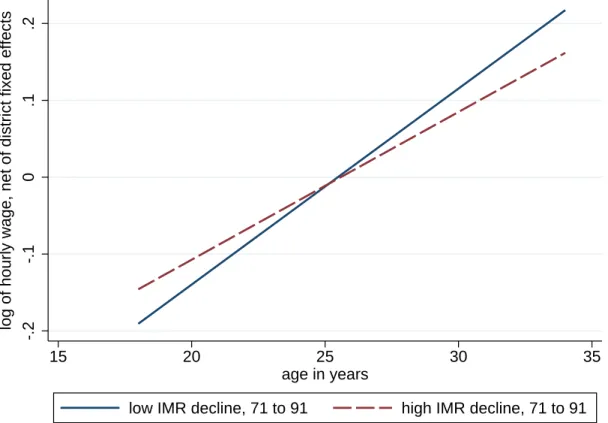
In particular, we match historical, district-level census data on the disease environment with cross-sectional survey data on adult wages. Figure 1 presents our identification strategy graphically. The graph plots average wages, net of district fixed effects, as a linear function of age. The most visible feature of the graph is the upward slope: within essentially all Indian districts, older workers are paid more than younger workers, on average.

Our identification is found in the difference between the two slopes. The average disease environment was better in 1990 than in 1970 in essentially all districts. However, these improvements were not uniform across districts. In districts where the disease environment improved more quickly over this period, younger workers would be expected to have rela- tively better early-life human capital than older workers in the same district, in comparison with the difference between older and younger workers in other districts where the disease environment improved more slowly. Therefore, our identification strategy asks whether the positive gradient between ages and wages is less steep in districts where the disease envi- ronment improved more quickly. An initial answer is visible in the difference in two slopes in Figure 1: the age profile of wages is less steep in the half of villages with above-average declines in infant mortality.

To quantify this effect, we estimate the following district-by-year differences-in-differences regression:

ln (y

) = βdisease

+ X

θ + α

+ γ

+ ε

(1) where i indexes individual adult workers, d denotes districts, and t represents years of birth.

We use district fixed effects α to control for any average differences in labor markets across

to geographic differences in average human capital. For example, if an improving disease environment in

the 1980s caused more factories to be built in a district in the 1990s, this change in labor demand would

be absorbed by the district fixed effect in our 2005 cross-section, insofar as it impacted workers of different

ages in our sample equally. If such endogenous demand responses are quantitatively important, then the

true positive effect of the early-life health environment on wages may be greater than our estimates.

districts, and year fixed effects γ to account for the overall age profile of wages. Standard errors are clustered conservatively at the district level, clustering all individuals in a district regardless of their year of birth or within-district primary sampling unit. We include district fixed effects using within estimation, rather than least-squares dummy variables, to properly correct standard errors for the finite sample (Cameron and Miller, 2013).

To demonstrate the stability of our coefficient estimate and the robustness of our strategy, we add controls X

in stages:

• state-specific linear time trends: identifies the disease environment from the extent to which the district time trend in disease differs from the state-wide disease time trend, to rule out any spurious state-level omitted variables;

• state × urban fixed effects: controls for a separate rural-urban difference in each state;

• state × social group indicators: state-specific indicators for eight caste and religion groups;

• female literacy: district-level female literacy in the district and year of the man’s birth, matched from census data in the same way as are sanitation and IMR.

The control for female literacy – another indicator of human development and an important determinant of early-life human capital – helps ensure that we are identifying effects of the disease environment, and also verifies that no spurious coefficient is mechanically introduced by our district-level matching process.

We will additionally add two further sets of covariates which may entail overcontrolling, relative to a properly specified model, but which will allow us to further rule out omitted variable bias while investigating possible mechanisms of the effect we document. First, we will add indicators for the worker’s membership in seven job categories,

which rules out spurious structural differences in district labor markets. Finally, we will add detailed indicators for education-by-grade interacted with literacy. These additions would be overcontrolling if education or job categories were partially caused by early-life disease.

4

The seven categories are family (own) farm work, animal care, agricultural wage labor, non-agricultural

wage labor, a salaried job, work at a family business, and any other work (the omitted category).

Our strategy implicitly assumes that the young adult men in our sample were born in the same district in which they lived at the time of our data. This is a reasonable assumption, because permanent migration for adult males in India is relatively uncommon (Rosenzweig and Stark, 1989); in contrast, women often migrate at the time of marriage to join their husbands’ households.

Appendix A uses various numerical strategies to demonstrate that our result would not be likely to be importantly different if we knew the actual birth district of the adults in our sample, rather than the district in which they now live. In particular, excluding the small fraction of men who have ever moved residences does not meaningfully change our coefficient estimates.

2.2 Variables and Data Sources

We match data from two different sources. For our dependent variables and control variables, we use data on individual adult males from the India Human Development Survey (IHDS), a nationally representative 2005 cross-sectional survey of 40,000 households (Desai et al, 2007).

Our primary dependent variable is the log of hourly wages in rupees, as computed by the IHDS.

As an input to our welfare computations, we also compute the effect of the early-life disease environment on household consumption per capita.

For our independent variables, we use two measures of the disease environment, both standard in the existing literature. First, we present results using infant mortality rates (IMR): the number of deaths in the first year of life per 1,000 live births. Economic historians have long used infant mortality as a measure of the disease environment. Early-life infant mortality rates are increasingly well understood to be an important determinant of height in developing countries today (Bozzoli, Deaton, and Quintana-Domeque, 2009), and historically in now-rich European countries (Hatton, 2014).

Second, we use district-level sanitation rates, operationalized as the percent of households in a district who use a toilet or latrine, rather than defecating in the open. Early-life exposure to open defecation in India has

5

Even so, Cutler et al (2010) also document that, in the 1991 Census, only 7.5% of all rural residents live outside their district of birth.

6

In cases where a respondent is not paid an hourly wage, the IHDS computes one from detailed questions about earnings at all jobs and hours worked.

7

In a similar empirical strategy, Almond, Currie, and Herrmann (2012) have recently used state-by-year

variation in infant mortality rates in U.S. states to identify effects of the early-life disease environment on

adult health among future mothers.

recently been shown to predict childhood height (Spears, 2012c) and childhood cognitive achievement (Spears and Lamba, 2012).

We take this historical data from the Indian Census. Census data are available only at 10 year intervals (1971, 1981, 1991), so we interpolate between Census rounds in order to match the adults we study with the IMR and open defecation rate in their district, in the year of their birth. Our preferred interpolation between census rounds is linear, but results are robust to using log-linear interpolation, or instrumenting for linear interpolation with log-linear interpolation to reduce measurement error, as we will show. We are constrained to use a smaller, younger sample when studying the effect of early-life sanitation because sanitation data are not available in the 1971 census.

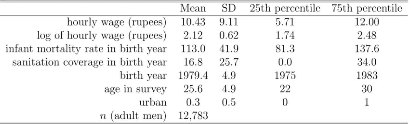
Table 1 presents summary statistics for the IHDS and census data that we use. Our av- erage workers are poor – earning about 10 rupees an hour – and were exposed to threatening early-life disease environments, with infant mortality of 113 deaths per 1,000 births and only about 17 percent sanitation coverage, on average. Because district-level census records are not available for IMR in the 1961 census, the workers we study are relatively young, with an average age of about 26 years.

3 Empirical Results

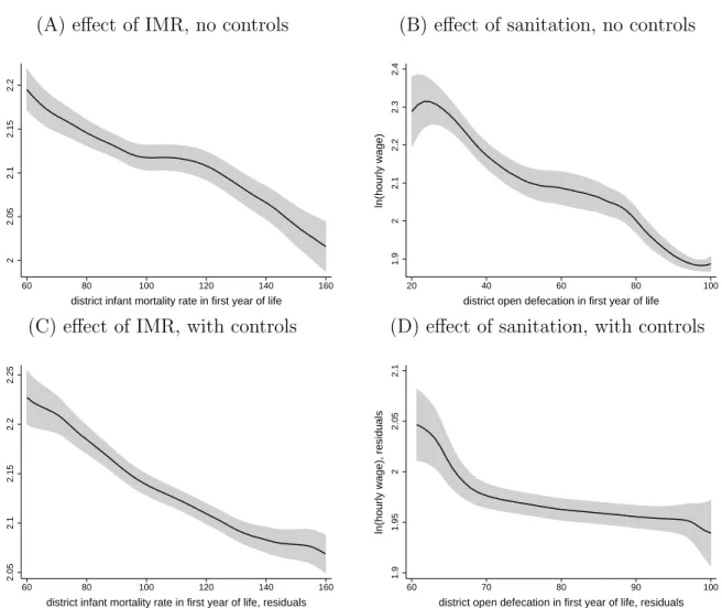
Figure 2 verifies that men who were born in district-years with worse infant mortality and sanitation earned lower wages as adults in the IHDS in 2005. Panels A and B plot locally weighted kernel regressions depicting a clear downward trend. Of course, wages are different, on average, in different places and for different age groups, for reasons other than effects of disease. Therefore, Panels C and D plot residuals of wages against residuals of our disease measures, in both cases after controlling for year-of-birth and state-times-urban fixed effects.

The visible downward trend remains, in an initial suggestion of the effect we will estimate.

8

Although latrines are a normal good, more likely to be owned by richer people, we are studying district-

level sanitation rates, which are not well explained by wealth in South Asia. Even the richest people in India

live near people who defecate in the open (Spears, 2013), which would have been even more the case in the

1970s and 1980s. Moreover, open defecation is not identical to failure to own a latrine: many, many people

in rural India choose to defecate in the open despite owning a latrine, perhaps provided by the government or

bought for the use of some members of the household, and certainly despite being able to afford one (Coffey

et al, 2014). Exposure to open defecation in South Asia is not a mere proxy for socioeconomic status.

3.1 Measuring Disease with Infant Mortality

Table 2 verifies the quantitative robustness and statistical significance of our main empirical result: men who were born in district-years with higher infant mortality have lower adult wages, on average. The regression coefficients imply that a 1 percentage point increase in infant mortality (10 IMR deaths per 1,000) would be associated with a decline in adult wages of 1.7 percent or more.

The result is notably stable across regression specifications.

In particular, similar results are found if IMR is interpolated between survey rounds linearly, as in Panel A, or if linear interpolation is instrumented for with log-linear interpolation, as in Panel B, to reduce measurement error.

Adding a long vector of regression controls fails to importantly change the coefficient estimate. In particular, column 2 controls for state-specific linear year-of-birth trends (age gradients), separate urban indicators for each state, and separate religious and caste indi- cators for each state; the coefficient remains essentially identical, and if anything slightly increases. Columns 3 and 4 go further by controlling in a flexible semi-parametric way for variables which may well be in part consequences of early-life health and human capital accu- mulation: job categories and education, measured as school-grade indicators interacted with literacy. Neither of these coefficients importantly changes the coefficient on early-life IMR exposure. This suggests both that education and job categories are not omitted variables that are spuriously responsible for our main result and that early-life health does not appear to have its effect on wages through the mechanism of sorting into these categories.

3.2 Measuring Disease with Sanitation

Table 3 reports regression results substituting sanitation coverage for infant mortality as the independent variable. The sample is smaller in Table 3 than in the IMR analysis because historical sanitation data are not available as early as are historical IMR data; this smaller sample will decrease the precision of coefficient estimates. Insofar as results using sanitation

9

Cameron and Miller (2013) propose a strategy for two-dimensional clustering of standard errors: in

our case, by districts, and by age cohorts. When we implement this procedure, the standard error in

IMR decreases, although the number of birth cohorts in our study may be too small for credible asymptotic

estimates. We will not further discuss multi-dimensional clustering, and note here merely that this procedure

gives no reason to suspect that our standard errors are too small.

are broadly similar to results found using IMR, we interpret this concordance as indicative that the mortality results are indeed effects of the disease and health environment, rather than some other spurious correlate of IMR.

As the table shows, we indeed find effects of important but plausible magnitude of san- itation on adult wages. The dependent variable is the percent of households using a toilet or latrine, rather than defecating in the open. A 10 percentage point decrease in open defe- cation translates into an approximately 2-3 percent increase in wages. In the context of our identification strategy, we find that in districts where sanitation has improved more quickly over time, the within-district wage profile is less steeply increasing in age. As before, our result is quantitatively stable as a long vector of controls is added, including for state-specific time trends, caste and religious groups, and state-specific urban residence. Also as before, adding job categories and education indicators – although these are, themselves, predictive of wages – does not change the coefficient on early-life sanitation.

3.3 Assessing Plausibility of Effect Sizes

This section considers whether our coefficient estimates are of plausible size. Although no comparable estimates exist in the literature, we can make an approximate guess of a plausible magnitude of the effect we estimate by multiplying quantities that do exist in the literature:

%∆y

∆open defecation = ∆height (sd)

∆open defecation × ∆height (cm)

∆height (sd) × %∆y

∆height (cm) , (2) where height (cm) is adult height in centimeters and height (sd) is child height-for-age in stan- dard deviations. We assume that a one standard deviation increase in child height becomes a one standard deviation increase in adult height, and substitute 6.9 cm for

height (cm)

∆

height (sd) , the standard deviation of Indian adult male height in the most recent Demographic and Health Survey. We combine three estimates of

∆

height (cm) from the literature: Vogl’s (2014) from Mexico, and high and low estimates for men in the U.S. from Case and Paxson (2008). We use five estimates of

height (sd)

∆

open defecation : Lin et al (2013) from Bangladesh, Kov et al (2013) from Cambodia, and one estimate from Spears (2012a) and two from Spears (2013) from India.

10

The full set of quantities used is available upon request.

Crossing these produces 15 predictions of the coefficient for wages regressed on early-life sanitation coverage. These range from 0.0006 to 0.0052, with a median of 0.0017 and a 75th percentile of 0.0021. This is exactly the neighborhood of our estimates in Table 3: 0.0018 to 0.0032. Although our estimates are slightly above the median of these estimates, there is reason to suspect our estimate would be larger: a higher fraction of the variation in height in India reflects early-life health than in the U.S. or likely even than in Mexico. Indeed, Spears (2012b) finds that the gradient between height and cognitive achievement is much steeper for Indian children than for U.S. children. Therefore, we conclude that our estimates are quantitatively consistent with predictions from estimates in the literature.

3.4 Does Education Mediate the Effect?

Improved early-life health could increase adult human capital by increasing physical strength or cognitive ability directly, or by increasing attained schooling, which would in turn increase wages. However, in the regressions of wages on IMR and sanitation, although education sta- tistically significantly predicted wages, controlling non-parametrically for indicators for years of schooling interacted with literacy did not change the coefficient on IMR or sanitation. This suggests that early-life health is uncorrelated with attained schooling. This non-result makes less likely certain potential omitted variable threats, such as coincidental other improvements in education or human capital facilities in the same districts.

Table 4 verifies that neither IMR nor sanitation in the first year of life predicts either years of schooling or a binary indicator of literacy, after district and year fixed effects. As Card (2001) showed, if schooling and ability are complements, then optimizing households will allocate more schooling to higher ability children. It may appear paradoxical, therefore, that men in our sample who received better early-life health did not receive more schooling.

However, Cutler et al (2010), also studying India, similarly found that although reducing early-life exposure to malaria increased adult consumption, it did not improve literacy or primary school completion.

In India of the 1970s and 1980s, education may have been allocated by an alternative process of social hierarchy rather than to optimize human capital (Borooah and Iyer, 2005;

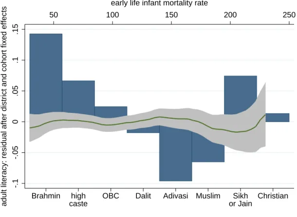
Thorat and Neuman, 2012). Figure 3 provides evidence that this may have occurred, using

the same sample as in the IMR estimates. The dependent variable, on the vertical axis, is the residual of literacy after district and year of birth fixed effects. The graph has two horizontal axes: IMR in the first year of life, along the top, and categories of caste and religion, along the bottom. The local kernel regression plots the association between the literacy residual and IMR: there is no relationship, and the prediction is never statistically significantly different from zero. In contrast, there are large differences in literacy according to caste and religious groups. It appears that social groups and hierarchy – much more than ability as shaped by early-life disease – shaped the allocation of education for Indian men of the cohorts studied. If social hierarchy indeed limited the ability of the Indian economy to optimally allocate investments in human capital, then the effects of early-life health on adult wages that we estimate may be less than the effects that would have been otherwise possible.

3.5 Controlling for Historical Female Literacy

We have shown a robust association between the early-life disease environment and adult wages that does not appear to spuriously reflect other time trends, correlated effects of con- temporary labor markets, adult occupation, educational achievement, or social heterogeneity.

Could our result, however, merely reflect a different dimension of the early-life environment?

Although many dimensions of heterogeneity in historical Indian districts have already been accounted for by our empirical strategy, here we focus on a particular measure of human development that is available in historical census data, important for child human capital accumulation, and distinct from the disease environment: average levels of female literacy.

This method has the further advantage of being a verification of our technique of interpo- lating independent variables from historical census data; in other words, similarly construct- ing an additional variable from similar historical sources helps us verify that the association we find with adult wages is not mechanically implied by our procedure (although there is no particular reason to suspect this). Therefore, we construct district level annual time series of female literacy by interpolating linearly between census rounds, and match adult males in the IHDS with district level female literacy in the year of their birth.

Table 5 presents results of adding female literacy to our analysis. Column 1 first checks

the plausibility of the female literacy data by showing that it is, as expected, positively associated with sanitation and negatively associated with IMR from the same district-year, with district and year fixed effects. The remaining columns replicate our main regression results and show that the coefficient is essentially unchanged with the addition of female literacy. Historical female literacy is not available for every district year; column 3 shows that restricting the sample to the observations with female literacy does not change our result.

Column 4 shows that adding a control for female literacy does not change the coefficient on sanitation or IMR, and column 5 confirms that this remains true with the full set of regression controls.

Therefore, the stability of our estimates again support our interpretation of an effect of early-life disease exposure on adult economic outcomes.

3.6 Effects of IMR on Consumption

Estimating the effect of the early-life disease environment on consumption is an important extension for two reasons. First, it is a robustness check of our main results: we would expect an increase in income to increase household consumption, especially if the adult male we study is an important source of household income. Second, consumption taxes – such as value added tax – are a larger fraction of government revenues in India than income tax, and thus if we are concerned about the fiscal impacts of the early-life disease environment, it is important to confirm that consumption is affected as well.

Table 6 presents effects of early-life IMR on the log of household monthly consumption per capita.

Column 1 repeats the estimate with controls of the effect of IMR on wages from Table 2; the effect on household consumption in column 2 is similar, although slightly smaller. Importantly, however, the adult men whom we are able to study are relatively young, and only some of them will be significant earners for their households. One common family structure in India is a joint household where adult men and their spouses live with the man’s parents; such households could have multiple brothers and a father earning income. Column

11

We note that in both samples female literacy in the year of birth is positively and statistically significantly associated with adult wages in a simple regression, but its coefficient changes sign to negative, as seen in the table, when district and year fixed effects and our measures of the disease environment are added. This is surprising, but is beyond the scope of our paper.

12

Because we only have sanitation data for very young workers, it is not feasible to estimate the effect

of sanitation coverage on consumption, as young workers play a small role in shaping their household’s

consumption. The results when we inappropriately attempt such a regression are inconsistent.

3 restricts the sample to the approximately two-thirds of the men we study who earn the most money of all people in their household; the effect is quantitatively similar to the effect on wages in column 1. Column 4 presents results for men who are not main earners; their early-life disease environment has no detectable effect on their households’ consumption.

This non-finding is important because it is consistent with what the economic demography of the Indian context would predict; this therefore suggests that our finding is not merely a spurious reflection of correlation between some aspect of households’ socioeconomic status today and the disease environment in their districts in past decades.

3.7 Further Robustness Checks

We present a further set of robustness checks in appendices A and B. First, in appendix A, we examine the sensitivity of our results to selective migration, by omitting individuals who have moved since birth, and we find that our results are essentially unchanged. Further analysis of the population which did move shows no evidence of any selective migration; if anything, high-skilled migrants seem to have been less likely to move to improved districts among younger workers.

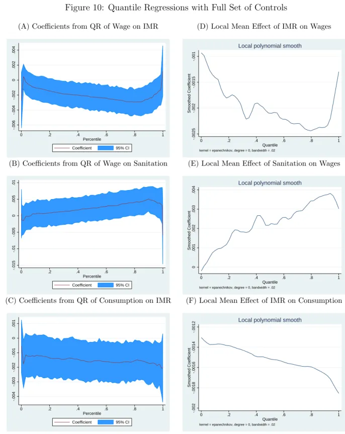
In appendix B, we present the results of a series of quantile regressions, which generally support our main conclusions: the coefficients tend to be of similar magnitudes to the OLS values, though with stronger effects towards the top of the distribution. We will discuss these findings further in our fiscal and welfare analysis.

4 Fiscal and Welfare Implications

Our analysis so far has produced coherent evidence that improvements in sanitation and in

the disease environment more broadly are associated with higher wages and consumption. As

a result, we expect that such improvements would have positive effects on the tax revenues

collected by the Indian government, and that the higher wages and consumption will translate

into increased utility for individuals and their households. In order to provide evidence on

the overall value of investments in improving sanitation and the disease environment, in this

section of the paper, we translate the empirical estimates from the previous section into

estimates of the fiscal and welfare gains from improvements in sanitation and the disease

environment.

We begin with the fiscal analysis, asking the question: if we could reduce the infant mortality rate by 1% point starting today, or if we could eliminate open defecation in India today, what would be the impact on the tax revenues collected by the Indian government as a result of higher wages? We then ask a similar question about the improvements in welfare for individuals resulting from higher consumption.

4.1 Fiscal Gains from Improved Sanitation & IMR

In the previous section, we demonstrated that improvements in sanitation and the dis- ease environment are associated with higher wages and consumption. An immediate corol- lary of these results is that investments in sanitation improvements will raise the tax rev- enues collected by the Indian government, through increased payments of both income and consumption-based taxes.

Given our estimates of the impact of sanitation and IMR on wages, and an approximation to the tax system in India, we can estimate the future gains in tax revenues above and beyond the “business-as-usual” value. Since these revenue gains oc- cur in the future, starting when the year-of-birth cohort born today enters the labor market, and gradually phasing in after that as more treated cohorts enter, we can use an appropriate discount rate to add up these future gains and express the revenue gains as a present-value equivalent.

For our main analysis, we use the linear regression results from Tables 2 and 3; we also use the quantile estimates found in appendix B to perform a robustness check in appendix C.1. As our baseline estimates, we use the values from column 1, where a 1% point increase in the IMR (or 10 points of IMR per 1000) is associated with 1.74% lower wages, while a 10% point increase in sanitation coverage is associated with 2.96% higher wages. These values are in the middle of the range of estimates, but we will also present results later with additional controls included.

We assume that the impact of sanitation and IMR on tax revenues is the same size: 1.74%

13

Only about 3% of the population of India pays income taxes, as the income threshold for paying tax is

set at 200000 rupees, several multiples of per-capita GDP. However, the quantile regressions in the previous

section indicate that the effect of sanitation and IMR on wages is larger at the upper end of the distribution,

meaning that it is reasonable to expect an impact on the wages of people paying income tax, as well as an

increase in the number of people earning enough to qualify.

and 2.96%. Given the results of the quantile regressions, this is likely to be a conservative assumption, as the impact is larger at higher incomes, where people are most likely to be paying taxes. We also limit our attention to the income tax and excise and service taxes, as these are taxes which depend directly or in a close indirect way on income and consumption; we ignore customs duties as well as the corporate tax, even though one might expect more productive workers to lead to larger corporate profits. The revenue from these taxes amounted to about 5.11 trillion rupees in 2012-13, or $93.64 billion US.

We assume that individuals have 40 years of working life, and that in the business-as- usual scenario each year-of-birth cohort produces an equal share of the tax revenue, or $2.34 billion per cohort. This is another conservative assumption, as we ignore economic growth and population growth, and in particular we ignore the possibility that younger cohorts, being better educated, earn more even in the business-as-usual scenario. We use a discount rate of 3.81%, which is the real interest rate facing the government as of February 2014 (an 8.86% interest rate on 10-year bonds minus 5.05% inflation). We then use this discount rate to add up the revenue gains from two separate interventions: a 10 point, or 1% point, reduction in the infant mortality rate starting today and continuing for the next 100 years, and the elimination of open defecation today.

4.1.1 Fiscal Gains from 1% Point Reduction in IMR

In this analysis, we assume that the infant mortality rate drops by 1% point below the business-as-usual level today and for the next 100 years. This will start to produce fiscal gains 18 years from now when the first treated year-of-birth cohort enters the labor market;

those gains will phase in until 57 years from now when all workers in the labor market will have received the treatment, at which point revenues will be $1.63 billion higher than in the business-as-usual scenario, and will end 157 years from now when the last treated cohort leaves the labor market.

A 1% point reduction in the IMR is associated with a $41 million increase in tax revenues for each treated year-of-birth cohort, and by simply discounting and adding up these gains over the next 157 years, we find that the sum of the revenue increases is equivalent to $10.95

14

We use an exchange rate of $1 US = 54.5481 rupees, which was the average during the 2012-13 fiscal

year.

billion in present value terms.

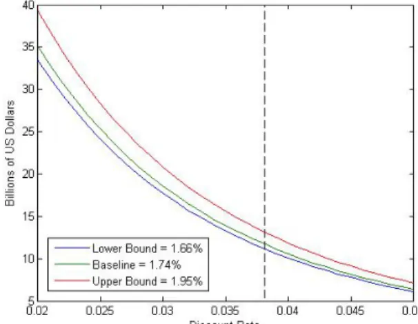
As a sensitivity analysis, we have also evaluated the revenue gains for the highest and lowest estimates in Table 2, and for a range of values for the discount rate; the results are displayed in panel (A) of Figure 4. Since the estimated effects of IMR on wages are close to each other, the three lines in the figure are very similar, but the revenue gain depends to a large extent on the discount rate, ranging from about $6-7 billion with a rate of 5% to as much as $39 billion with a 2% discount rate. The black dotted line in the figure shows the baseline discount rate of 3.81%.

In appendix C.1, we instead use our quantile regression estimates to calculate the increase in tax revenues, and find an even larger estimate of $15.94 billion, as might be expected from our observation that the impacts on wages appear to be strongest towards the top of the distribution.

4.1.2 Fiscal Gains from Eliminating Open Defecation

Next, we consider the impact of eliminating open defecation today. In 2011, it is estimated that 53.1% of Indian households defecated in the open, but that number had been declining at an average rate of 1.05 percentage points per year over the previous decade. Therefore, in our business-as-usual scenario, we assume that open defecation continues to decline at this linear rate in the future, so that absent any intervention open defecation would be eliminated in about 50 years. We assume linear gains from eliminating open defecation, so that each percentage point reduction in open defecation raises average wages by 0.296% from the current level, and thus raises tax revenues by $6.9 million per year-of-birth cohort.

Once again, the revenue gains begin 18 years from now, at $368 million, and gradually phase in until peaking at $9.04 billion per year 57 years from now. When aggregated up using a discount rate of 3.81%, we find a total present-value revenue gain of $60.48 billion. If we further divide this total by the number of households currently estimated to defecate in the open, which is approximately 131 million, we find that the revenue increase is $462 per household that is induced to stop defecating in the open. In panels (B) and (C) of Figure 4, the range of values generated by trying different discount rates and using the upper and lower bounds from Table 3 are displayed; the gains per household are around $200 at the

15

Alternatively, present-value government revenue increases by about $1 billion in response to a reduction

in IMR by one point on demographers’ traditional scale of deaths per thousand births.

low end and over $1000 at the top end.

This baseline result implies that investments in reducing or eliminating open defecation that cost less than $462 per household that stops defecating in the open would not have any net cost to the government; without any change in tax rates, the future tax revenues obtained above and beyond the business-as-usual value would be more than enough to pay for the original investment, even once those gains are discounted to account for the fact that they take 18 years to start being realized. In other words, the first $462 per household that is spent on eliminating open defecation is free from the perspective of the government.

Furthermore, on top of the numerous conservative assumptions made earlier, we have ignored other potential sources of fiscal gains, such as reduced public health care expenditures and calorie requirements if sanitation investments lead to improvements in health among the affected population.

In appendix C.1, we again use our quantile regression estimates to provide a robustness check on our estimated fiscal gains, and arrive at a present-value gain of $103.49 billion, or $790 per household that stops defecating in the open. It makes sense that results using quantile regressions are larger, because the quantile regressions suggested a bigger effect on richer workers. Our baseline estimates, therefore, appear to be lower bounds for the effects of early-life health on tax revenues.

4.2 Welfare Gains from Improved Sanitation and IMR

Increases in wages from improved early-life health not only raise tax revenues; they should also lead to higher after-tax wages and consumption, with resulting increases in utility. We now attempt to quantify these utility gains, counting only the gains from higher consumption;

as throughout the paper, we ignore all other benefits of better health and more physically and mentally capable citizens. We will focus on our regressions of wages on IMR and sanitation in Tables 2 and 3, as in our fiscal analysis, and use them to compute effects on after-tax wages. In appendix C.2, we also use our consumption regression estimates from Table 6, as well as the quantile regression estimates for both wages and consumption.

To quantify the gains in utility, we must present a basic model of individual utility; we

then solve the model for a simple expression for welfare which depends only on empirically

estimable coefficients, in the spirit of the “sufficient statistics” method of policy analysis discussed in Chetty (2009). We start with the assumption that individuals today receive some utility from toilet or latrine use d ∼ F (d), which could be positive or negative. Then the fraction L of people who use a latrine is defined by L = 1 − F (0), and we assume that for a cost of p per unit, the government can shift L upwards; essentially, we assume that through direct provision of a latrine and/or education or other activities to raise people’s tastes for latrine use, the government is able to take some individuals with negative d and shift them to indifference. In so doing, we ignore any welfare gains of this education on the utility of inframarginal latrine users; for example, while it is possible that community education programs could make people currently using a latrine feel happier about doing so, we have no way to measure this impact and so we ignore it. We also ignore any changes in taxes today, by assuming that if the tax rate needs to change to balance the budget, it will do so in the future for the taxes applied to the affected generations.

The result of this is that we can ignore the utility impact of the sanitation investment on the current generation, and focus only on the gains to future generations from higher wages and consumption. Begin by considering a single cohort of individuals born today, each facing the average sanitation coverage. Assume that each individual receives an income y

which is constant over time and is the sum of an idiosyncratic component x

∼ G(x) and a component that depends directly on the open defecation rate: y

= x

+ αL. Individuals obtain utility from consumption according to a CRRA utility function, U =

, and the government levies a tax on income T (y) and provides a lump-sum transfer b.

Consumption is thus c = y − T (y) + b, and if we assume that the budget constraint is balanced through changes in b, the effect of changing L on utility is:

dU

dL = c

(1 − t(y))γy + db dL

where γ =

=

dy y

dL

is the percentage increase in wages for a unit increase in L, as estimated earlier. Now consider that the cohort in question begins working at time t

and leaves the labor market at time t

, and that future utilities are discounted using some discount factor

16

In this environment, a tax on consumption is implicitly a tax on income; the point is to account for the

fraction of income that is paid in one tax or another.

β. Then, using a utilitarian social welfare function V = P

t=t0

β

E(U), the total welfare impact on this cohort is:

dV

dL = B (t

, t

)E

c

(1 − t(y))γy + db dL

where B(t

, t

) = P

t=t0

β

= β

is the sum of discount factors over time. Finally, to put this in dollar terms, normalize by the average marginal utility E c

: dW

dL ≡

dV dL

E (c

) = B(t

, t

) E c

(1 − t(y))γy +

E (c

) .

For purposes of illustration, suppose the cohort under consideration is the only one affected by the intervention, and the only one for whom b changes. Then the government’s budget constraint is:

B(t

, t

)E(T (y)) = B(t

, t

)b + pL and we can differentiate to find:

B(t

, t

) dE (T (y))

dL = B (t

, t

) db dL + p and therefore

=

−

0,t1)

. Then the welfare derivative is:

dW

dL = B(t

, t

) E

c

(1 − t(y))γy

E (c

) + B(t

, t

) dE(T (y)) dL − p.

This equation tells us something quite simple; notice that the second term is the discounted sum of increased tax revenues, while the third term is the cost of the intervention. These were the two terms of importance in the analysis of the fiscal impacts earlier. Therefore, to estimate the welfare impact of higher wages, we merely need to add to the net fiscal impact the discounted gains in after-tax income or consumption, weighted by marginal utility if there are any distributional impacts.

For the purpose of this analysis, we will focus on a fiscally neutral improvement in

sanitation or IMR; although the model is in terms of open defecation, we can easily reinterpret

L as the infant mortality rate and the same equation applies. Therefore, we consider an

investment costing $10.95 billion per 1% point reduction in IMR, or $462 per household

induced to stop defecating in the open. Furthermore, we ignore any distributional effects

and look at the impact on an average individual; distributional effects are considered in appendix C.2. Specifically, we consider the impact on an individual receiving the average per-capita income of $1219. Tax revenue was estimated to be 10.39% of GDP in 2011, according to the World Bank, so we use a net-of-tax rate of 0.8961, and we continue to use 3.81% as the annual discount rate, although now this should be understood as either a personal or social rate of time preference.

4.2.1 Welfare Gains from 1% Point Reduction in IMR

Given the assumptions above, each 1% point reduction in IMR raises wages by $21 per male worker per year. As a result, using the estimated male population of main workers from the 2011 Census, totalling about 273 million, the present-value increase in welfare amounts to $37.27 billion, or over three times the fiscal gains. Panel (A) of Figure 5 displays the robustness of this result to varying estimates and discount rates; they confirm a significant welfare gain that ranges from about $20 billion to over $120 billion. In appendix C.2, we estimate the welfare gain using the estimates from the regression of consumption on IMR in Table 6, as well as the estimates from quantile regressions of wages and consumption on IMR, and in each case we find even larger values than the baseline.

4.2.2 Welfare Gains from Eliminating Open Defecation

Our estimates above indicate that each 10% point reduction in open defecation raises wages by $36. This implies that the elimination of open defecation would generate total discounted gains of $1852 for an individual born today;

this is equivalent to about one and a half times the current GDP per capita, or about 12.4 years of maximal annual earnings from NREGA, a large government workfare program. Over the entire workforce, the total after-tax income gains are $192.7 billion; that is, the total increase in utility over the next 100 years or so from the income consequences of eliminating open defecation today is equivalent in present value terms to a helicopter-drop of $192.7 billion on the Indian population today. Figure 5 displays the robustness of these results; the gains are large at all combinations of parameters, and reach as high as about $476 billion in total, or $3649 per individual born today. Appendix

17

If discounting starts only at the time of the individual’s entry into the labor market 18 years from now,

the gain is a far larger $14239.

C.2 contains an estimation of this welfare gain using the quantile regression estimates of the effect of sanitation on wages, and we find an increased estimate of $2235 per household and

$232.6 billion at an economy-wide level in present value. Finally, to emphasize, all of these estimates of “utility” impacts refer only to utility from increased consumption, and not from any other benefits of improved health, cognitive achievement, or mortality.

5 Conclusion

This paper examines the effects of the early-life disease environment on adult wages, decades later. Exploiting heterogeneity across Indian districts in the time-paths of improvement in infant mortality and in sanitation, we find that men exposed to a better early-life disease environment earned significantly but plausibly higher wages as adults. The estimated gains are similar across a wide range of specifications and sets of fixed effects; are comparable across the mortality and sanitation results; and are consistent with finding improvements in consumption of similar magnitude, precisely when the man for whom we have data is the household’s main earner. These results are not spurious consequences of selective migration, which we can observe in our data. Our results are not driven by changes in education; this is consistent with evidence from Cutler et al (2010) on the effects of early-life malaria expo- sure on subsequent consumption in India, and with non-optimizing allocation of education in India’s caste hierarchical society (Thorat and Neuman, 2012). Moreover, the apparent unim- portance of education to the health-wages relationship may make certain omitted variable threats less likely, such as coincidental other improvements in education or other human capital facilities in the same districts. These findings suggest that early-life exposure to infectious disease could have an appreciable impact on economic outcomes in developing countries, at least in contexts such as India’s, where widespread open defecation is paired with high population density.

The relatively modest effects on wages that we estimate add up to important fiscal

consequences. Wage gains occur decades after improvements in the disease environment, so

the present-day benefit depends on the interest rate. Our baseline estimate, calibrated to the

interest rate at which the Indian government borrows money, finds that if the government

were to eliminate open defecation by spending up to $462 per household that defecates in the

open, such a program would impose no net present fiscal cost.

This number considers only the government’s revenue and therefore ignores any savings to the government on healthcare, as well as the large economic benefits to workers of the wages that they do not pay in taxes, and all non-economic benefits of better health. Of course, this result does not, itself, provide any advice to the Indian government about how to reduce open defecation; nor would there be any effect on wages of spending government revenue on an unsuccessful sanitation program.

However, our results indicate that public investments to change sanitation behavior and reduce open defecation – as well as investments in other mechanisms of reducing infant mortality – could improve well-being at a low net present cost to the government.

A Testing for Selective Migration

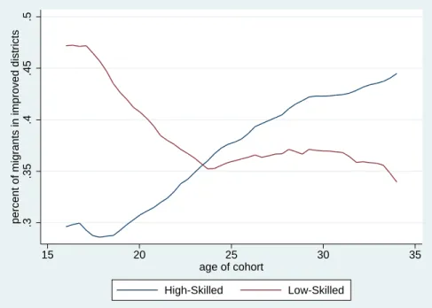
One possible factor that could be responsible for our findings is selective migration. It would require a fairly complicated migration pattern: it would have to be the case that higher-skill individuals among the younger cohorts net migrate selectively into districts where the disease environment improved the most, or out of districts where the disease environment did not improve. Therefore, wages among young workers in improved districts would be higher not because of any causal effects of the improved disease environment but rather because they are naturally more skilled workers.

Fortunately, the IHDS includes data on migration, so we can test this hypothesis. The data report whether a particular individual moved since their birth, though we cannot see where they migrated from, so we are likely to overstate migration as many moves would be within the same district. We run the regressions of wages on IMR and sanitation only for stayers, by omitting all individuals who report ever having moved. The results are presented in Table 7, and the coefficients are nearly unchanged. Therefore, selective migration does not appear to be responsible for our results.

We can further test to see if there is any evidence for selective migration at all. We divide the sample into two halves, with all districts above the median improvement in IMR in our sample period in one half (“improved districts”) and all districts below the median in the other (“non- improved districts”), and calculate total migrants in each half by age, smoothed over age using a local average. Then we examine the share of overall migrants going to improved districts by age.

If selective migration was occurring, we might expect that a greater share of migrants would be found in improved districts among the younger cohorts, but in Figure 6 we see that, if anything, the opposite has actually occurred, with a general tendency towards a smaller fraction of migration to improved districts among younger workers.

Next, we also divide our population into two halves: we regress wages on year-of-birth and district fixed effects, and place all individuals with above-median residuals in one half and those below the median in the other, as a proxy for high- and low-skill groups. We then ask: has there

18

Indeed, the government would make money if a successful program were less expensive than this!

19

Alternatively, and more likely since the districts with the biggest improvements in IMR and sanitation

tended to be districts with worse disease environments and lower wages both before and after our sample

period, we would have a problem if older high-skill workers net migrated to districts that did not see significant

improvements in disease environment.

been more high-skilled migration into improved districts relative to less-improved districts among young individuals? The results are presented in Figure 7, and once again the trend is, if anything, in the opposite direction: high-skilled migration as a fraction of total migration towards improved districts is lower for younger workers. Therefore, we can conclude that selective migration is not a problem for our analysis, because it does not appear to have occurred.

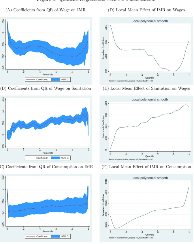
B Quantile Regressions

In this appendix, we ask the question: how does the impact of the early-life disease environment on wages or consumption vary across the ability distribution? The answer to this question will help us to further understand the way in which the disease environment interacts with other personal characteristics, and it is also of some importance for the fiscal and welfare analysis to come. If the impact is concentrated on high-ability (and thus typically high-income) individuals, for example, the effect on tax revenues is likely to be larger than would otherwise be the case, whereas the welfare impact may be smaller because of increased inequality.

We can answer this question using quantile regressions. Let us return to our original regression equation:

ln (y

) = βdisease

+ X

θ + ε

where X

is now a general set of controls, possibly including the year and district fixed effects.

For any percentile τ , the typical quantile regression

estimates the following:

ln (y

) = β

disease

+ X

θ

+ ε

.

where both β and θ are allowed to vary across the distribution. However, we prefer to think of the fixed effects and time trends contained in X

as constant additive components, which therefore would not vary across the distribution; therefore, we use the two-step procedure in Canay (2011) to estimate the following:

ln (y

) = β

disease

+ X

θ + ε

.

Canay’s procedure is simple: we perform an OLS regression of ln (y

) (wages or consumption) on disease

and a set of controls X

, and calculate ln (y ˆ

) = ln (y

) − X

θ, where ˆ ˆ θ is the estimated coefficient on X

. Then we perform a quantile regression of ln (y ˆ

) on disease

. The results are displayed in panels (A) through (C) of Figure 8, for the case in which X

contains only district and year-of-birth fixed effects; the blue bands represent 95% confidence intervals using bootstrapped standard errors.

The results are suggestive of a larger effect of the disease environment on wages towards the upper end of the distribution; the consumption estimates are flat and never attain statistical sig- nificance. However, the next question is: which distribution are we looking at? That is, which variable is distributed along the x-axis? Because the regressions condition on disease

and X

, the distribution in question is the distribution of ln (y

) controlling for disease

and X

, which is equivalent to the distribution of ε

; we are looking at the effect of the disease environment on wages and consumption at different points in the distribution of unobservables. Essentially, we are looking at the effect on individuals based on their place in the distribution of wages in their district and year of birth.

These results remain of interest, because although high and low-income workers are mixed together in the distribution of ε

, it is still true that on average, an individual who is near the top

20

For example, what we call the typical quantile regression is what qreg estimates in Stata.

of the distribution of unobservables will have a higher wage than someone near the bottom of the distribution. There are a few alternative strategies that we can use, however, that might allow us to say something about the effect along the current income distribution; one is to attempt to transform the coefficients by quantile on the distribution of ε

into average coefficients by quantile on the distribution of ln (y

). That is, by estimating the OLS regression of ln (y

) on disease

and X

, we can use the residuals as a proxy for ε

and thus assign each individual a coefficient β

based on their place in the distribution of residuals. Then, we can look at the distribution of β

across the wage or consumption distribution. In panels (D) through (F) of Figure 8, we present the smoothed local means of β

at quantiles of the wage or consumption distributions; given the ad-hoc nature of the calculation, we have not attempted to calculate standard errors, but the means confirm the results so far: the largest effects of the early-life disease environment on wages occur towards the upper end of the distribution. The same appears to be true of the consumption regression as well, though the lack of precision in the quantile estimates make the results less clear than in the wage case.

An alternative strategy is to remove some of the controls, and so in Figure 9, we present the results of quantile regressions without the district and year-of-birth fixed effects. The results are broadly similar to those in Figure 8, though the coefficients are larger, since they are now picking up part of the district and year fixed effects; the consumption estimates are also somewhat altered, in that they now show a larger effect near the bottom of the distribution. However, this approach is not entirely satisfactory, as the regression equation is now almost certainly misspecified, as the omitted fixed effects are surely correlated with both the disease environment and wages.

Finally, Figure 10 presents the results from quantile regressions with the full set of controls:

district and year-of-birth fixed effects, but also state × urban fixed effects, state time trends, and social group × urban indicators. The estimates are quite similar to those in Figure 8, though somewhat larger and more significant for consumption and smaller and less significant for sanitation.

C Robustness Checks on Fiscal and Welfare Calcula- tions

In this appendix, we produce alternative estimates of the fiscal and welfare impacts of improved sanitation and early-life disease environment. First, we examine the robustness of our estimates of the increased tax revenues resulting from improved sanitation or IMR, using the results of our quantile regressions. Then we examine how the welfare gains are affected by using either quantile estimates or our regression of consumption on IMR.

C.1 Fiscal Impacts Using Quantile Regressions

In appendix B, we discussed how our quantile regression estimates of the effect of IMR and sanita- tion on wages could be used to assign each individual in our sample an estimated coefficient. We now make use of these personalized coefficients to produce new estimates of the fiscal effects of the sanitation and disease environment.

Our baseline fiscal and welfare analysis is conducted using 2012-13 dollars, and so we first

rescale the incomes in our sample to be representative of the average in 2012. According to the

World Bank, GNI per capita in India in 2012 was 83026.8 INR; therefore, we multiply all incomes

by a constant to make the mean in our sample 83026.8. Then, to account for the fact that we have