On the Geometry of Data Representations

Research Collection

Doctoral Thesis

On the Geometry of Data Representations

Author(s):

Bécigneul, Gary Publication Date:

2021

Permanent Link:

https://doi.org/10.3929/ethz-b-000460877

Rights / License:

In Copyright - Non-Commercial Use Permitted

This page was generated automatically upon download from the ETH Zurich Research Collection. For more information please consult the Terms of use.

O N T H E G E O M E T R Y O F D ATA R E P R E S E N TAT I O N S

A thesis submitted to attain the degree of d o c t o r o f s c i e n c e s o f e t h z u r i c h ¨

(Dr. sc. ETH Z ¨urich)

presented by g a r y b e c i g n e u l ´ Master in Mathematics University of Cambridge

born on 11 . 11 . 1994 citizen of France

Accepted on the recommendation of Prof. Dr. Thomas Hofmann (ETH Z ¨urich)

Prof. Dr. Gunnar R¨atsch (ETH Z ¨urich) Prof. Dr. Tommi Jaakkola (MIT)

Prof. Dr. Regina Barzilay (MIT)

2021

The vast majority of state-of-the-art Machine Learning (

) methods nowadays internally represent the input data as being embedded in a

“continuous” space, i.e. as sequences of floats, where nearness in this space is meant to define semantic or statistical similarity w.r.t to the task at hand. As a consequence, the choice of which metric is used to measure nearness, as well as the way data is embedded in this space, currently constitute some of the cornerstones of building meaningful data representations.

Characterizing which points should be close to each other in a given set essentially defines a “geometry”. Interestingly, certain geometric properties may be incompatible in a non-trivial manner − or put an- other way, selecting desired geometric properties may have non-trivial implications. The investigation of which geometric properties are de- sirable in a given context, and how to enforce them, is one of the motivations underlying this thesis.

Initially motivated by uncovering how Convolutional Neural Net- work (

) disentangle representations to make tangled classes linearly separable, we start our investigation by studying how invariance to nuisance deformations may help untangling classes in a classification problem, by locally contracting and flattening group orbits within data classes.

We then take interest into directly representing data in a Riemannian space of choice, with a particular emphasis on hyperbolic spaces, which is known to be better suited to represented tree-like graphs. We develop a word embedding method generalizing G lo V e , as well as a new way of measuring entailment between concepts. In the hyperbolic space, we also develop the tools needed to build neural networks, including matrix multiplication, pointwise non-linearity, Multinomial Logistic Regression (

) and Gated Recurrent Unit (

).

Since many more optimization tools are available for Euclidean do-

mains than for the hyperbolic space, we needed to adapt some of the

most powerful adaptive schemes − A dagrad , A dam , A msgrad − to

such spaces, in order to let our hyperbolic models have a chance to

outperform their Euclidean counterparts. We also provide convergence

for the particular case of the Euclidean space.

Finally, the growing prominence of graph-like data led us to extend some of the most successful Graph Neural Network (

) architectures.

First, we start by generalizing Graph Convolutional Network (

)s to hyperbolic and spherical spaces. We then leveraged Optimal Trans- port (

) geometry to turn current architectures into a universal ap- proximator, by dispensing with the last node aggregation step yielding the final graph embedding.

We hope that this work will help motivate further investigations in

these geometrically-flavored directions.

La grande majorit´e des m´ethodes d’Apprentissage Automatique (

) atteignant l’´etat-de-l’art de nos jours repr´esente les donn´ees rec¸ues en entr´ee dans un espace “continu”, i.e. comme une s´equence de nombres d´ecimaux, dans un espace o `u la proximit´e est vou´ee `a d´efinir la similarit´e s´emantique ou statistique par rapport `a la tˆache. En cons´equence, le choix de la m´etrique utilis´ee pour mesurer la proximit´e, ainsi que la fac¸on dont les donn´ees sont plong´ees dans cet espace, constituent actuellement l’une des pierres angulaires de l’´edification de bonnes repr´esentations des donn´ees.

Charact´eriser quels points doivent ˆetre proches les uns des autres dans un ensemble d´efinit essentiellement ce qu’on appelle une g´eometrie.

Il se trouve que certaines propri´et´es g´eom´etriques peuvent ˆetre incom- patibles d’une fac¸on non-triviale − ou, dit autrement, la s´election de cer- taines propri´et´es g´eom´etriques peut avoir des implications non-triviales.

La recherche de quelles propri´et´es g´eom´etriques sont souhaitables dans un contexte donn´e, et de comment les obtenir, est l’une des motivations principales sous-jacentes `a cette th`ese.

Initiallement motiv´e par la d´ecouverte de comment les r´eseaux de neurones `a convolutions parviennent `a d´esenchevˆetrer les donn´ees afin de rendre des classes enchevˆetr´ees linearement s´eparables, nous commenc¸ons notre recherche en ´etudiant comment l’invariance `a des transformations nuisibles peut aider `a d´esenchevˆetrer les classes d’un probl`eme de classification, en contractant et en applatissant locallement des orbites de groupes au sein des classes de donn´ees.

Nous nous int´eressons ensuite `a repr´esenter directement les donn´ees dans un espace Riemannien de choix, avec une emphase particuli`ere sur les espaces hyperboliques, qui sont connus pour ˆetre mieux adapt´es

`a repr´esenter les graphes ayant une structure arborescente sous-jacente.

Nous d´eveloppons une m´ethode de word embedding g´en´eralisant G lo V e ,

ainsi qu’une nouvelle fac¸on de mesurer les relations asym´etriques

d’inclusion s´emantique entre les conceptes. Nous d´eveloppons ´egalement

les outils n´ecessaires `a la construction de r´eseaux de neurones dans

les espaces hyperboliques: multiplication matricielle, application de

non-lin´earit´e ponctuelle, r´egression multi-logistique et

.

espaces Euclidiens que pour les espaces hyperboliques, nous avions besoin d’adapter certaines des m´ethodes adaptives les plus perfor- mantes − A dagrad , A dam , A msgrad − `a ces espaces, afin de per- mettre `a nos mod`eles hyperboliques d’avoir une chance de performer sup´erieurement `a leur analogue Euclidien. Nous prouvons ainsi des garanties de convergence pour ces nouvelles m´ethodes, qui recouvrent celles d´ej`a connues pour le cas particulier de l’espace Euclidien.

Enfin, la pr´esence accrue de donn´ees sous forme de graphe nous a conduit `a ´etendre certaines des architectures de r´eseaux de neurones de graphes les plus puissantes. En premier lieu, nous commenc¸ons par g´en´eraliser les r´eseaux de neurones de graphes `a convolutions, aux espaces hyperboliques et sph´eriques. Ensuite, nous faisons appel

`a la g´eom´etrie du transport optimal pour transformer les architec- tures courantes en approximateur universel, en supprimant la derni`ere aggr´egation des repr´esentations internes des noeuds du graphe qui avant r´esultait en la repr´esentation finale du graphe.

Nous esp´erons que ceci contribuera `a motiver davantage d’explorations

dans ces directions de recherche `a tendance g´eom´etrique.

The material presented in this thesis has in parts been published in the following publications:

1 . Octavian-Eugen Ganea

, Gary B´ecigneul

and Thomas Hofmann.

“Hyperbolic Neural Networks.”

NeurIPS

Advances in Neural Information Processing Systems.

[GBH

2 . Gary B´ecigneul and Octavian-Eugen Ganea.

“Riemannian Adaptive Optimization Methods.”

ICLR

International Conference on Learning Representations.

[BG

].

3 . Alexandru Tifrea

, Gary B´ecigneul

and Octavian-Eugen Ganea

.

“Poincar´e GloVe: Hyperbolic Word Embeddings.”

ICLR

International Conference on Learning Representations.

[TBG

].

4 . Gregor Bachmann

, Gary B´ecigneul

and Octavian-Eugen Ganea.

“Constant Curvature Graph Convolutional Networks.”

ICML

International Conference on Machine Learning.

[BBG

].

In part currently under review:

5 . Gary B´ecigneul

, Octavian-Eugen Ganea

, Benson Chen

, Regina Barzilay, Tommi Jaakkola.

“Optimal Transport Graph Neural Networks.”

Under Review at ICLR

[B´ec+

].

And in part unpublished:

6 . Gary B´ecigneul.

“On the Effect of Pooling on the Geometry of Representations.”

arXiv preprint arXiv:1703.06726,

[B´ec

].

1Equal contribution.

results that are supplemental to this work or build upon its results, but are not covered in this dissertation:

7 . Octavian-Eugen Ganea, Gary B´ecigneul and Thomas Hofmann.

“Hyperbolic Entailment Cones for Learning Hierarchical Em- beddings.”

ICML

International Conference on Machine Learning . [GBH

8 . Octavian-Eugen Ganea, Sylvain Gelly, Gary B´ecigneul and Aliak- sei Severyn.

“Breaking the Softmax Bottleneck via Learnable Monotonic Point- wise Non-linearities.”

ICML

International Conference on Machine Learning.

[Gan+

].

9 . Ondrej Skopek, Octavian-Eugen Ganea and Gary B´ecigneul.

“Mixed-Curvature Variational Autoencoders.”

ICLR

International Conference on Learning Representations.

[SGB

].

10 . Foivos Alimisis, Antonio Orvieto, Gary B´ecigneul and Aur´elien Lucchi.

“A Continuous-time Perspective for Modeling Acceleration in Riemannian Optimization

AISTATS

International Conference on Artificial Intelligence and Statistics.”

[Ali+

11 . Calin Cruceru, Gary B´ecigneul and Octavian-Eugen Ganea.

“Computationally Tractable Riemannian Manifolds for Graph Embeddings.”

AAAI

Association for the Advancement of Artificial Intelligence.

[CBG

].

Currently under review are also other parts of my PhD research and present results that are supplemental to this work or build upon its results, but are not covered in this dissertation:

12 . Louis Abraham, Gary B´ecigneul, Benjamin Coleman, Anshumali

Shrivastava, Bernhard Sch ¨olkopf and Alexander J Smola.

Under Review at AISTATS

[Abr+

].

13 . Foivos Alimisis, Antonio Orvieto, Gary B´ecigneul and Aur´elien Lucchi.

“Practical Accelerated Optimization on Riemannian Manifolds.”

Under Review at AISTATS

[Ali+

Finally, the following pieces of work were also part of my PhD research but remained unpublished:

14 . Gary B´ecigneul, Yannic Kilcher, Thomas Hofmann.

“Learning a Riemannian Metric with an Energy-based GAN.”

Unpublished.

[BKH

].

15 . Yannic Kilcher

, Gary B´ecigneul

, Thomas Hofmann.

“Escaping Flat Areas via Function Preserving Structural Net- work Modifications.”

OpenReview preprint openreview:H1eadi0cFQ,

[KBH

].

16 . Yannic Kilcher

, Gary B´ecigneul

, Thomas Hofmann.

“Parametrizing Filters of a CNN with a GAN.”

arXiv preprint arXiv:1710.11386,

[KBH

].

First, I thank my professor Thomas Hofmann for the continuous support during my PhD studies at ETH. His trust in my success and the provided scientific freedom and guidance were decisive to the result of this thesis. Next, I would also like to express my gratitude to Octavian-Eugen Ganea, with whom I brainstormed almost daily.

I am also very grateful to Tommi Jaakkola and Regina Barzilay who warmly welcomed me in their lab to work with them at MIT, showed me new problems and inspired me, and to Benson Chen who also worked with us.

Many thanks to Bernhard Sch ¨olkopf for thinking about me to help design a group testing method and for his close collaboration; to Louis Abraham for solving non-trivial problems on a short notice, and Ben Coleman, Anshumali Shrivastava and Alexander Smola in this team work.

I would also like to acknowledge my co-workers during this PhD:

Alexandru Tifrea, Gregor Bachmann, Foivos Alimisis, Antonio Orvi- eto, Aurelien Lucchi, Andreas Bloch, Calin Cruceru, Ondrej Skopek, Sylvain Gelly, Yannic Kilcher, Octav Dragoi, Philipp Wirth, Panayiotis Panayiotou, Charles Ladari, Severin Bahman, Jovan Andonov, Igor Petrovski, Gokul Santhanam, Yashas Annadani, Aliaksei Severyn, and all my Data Analytics Lab, CSAIL and MPI colleagues. Thank you!

I am especially grateful to Gr´egoire Fanneau who gave birth to my interest for mathematics in high school, to Prof. Jean-Claude Jacquens and to Prof. Luc Albert, who taught me mathematics and computer science and challenged me in French preparatory classes. Also, many thanks to Simon Janin for bringing light to the blindspots present in my workflow and for coaching me over the years. Thanks to R´emi Saidi for increasing my standards of mathematical rigor. Thanks to Victor Perez, Nicole and Dominique Secret for believing in me and supporting my undergraduate studies.

Last but not least, all my love to my mother for her encouragement, trust and support from day one.

I dedicate all my work to my little brother, Tom B´ecigneul, who left

us too early, but whose joy of life continues to inspire me.

a c r o n y m s

1 i n t r o d u c t i o n , m o t i vat i o n s & g oa l s

1 . 1 A Primer on Machine Learning . . . .

1 . 2 Euclidean Representations . . . .

1 . 2 . 1 Power & Ubiquity . . . .

1 . 2 . 2 Limitations . . . .

1 . 3 Beyond Euclidean Geometry . . . .

1 . 3 . 1 Characterizing the Geometry of Discrete Data . .

1 . 3 . 2 Non-Euclidean Properties of Data Embedded in a Euclidean Space . . . .

1 . 3 . 3 Hyperbolic Representations . . . .

1 . 3 . 4 Riemannian Optimization . . . .

1 . 3 . 5 Graph-like Data . . . .

1 . 4 Thesis Contributions . . . .

2 g r o u p i n va r i a n c e & c u r vat u r e o f r e p r e s e n tat i o n s

2 . 1 Background Material . . . .

2 . 1 . 1 Groups, Lie Algebras & Haar Measures . . . .

2 . 1 . 2 I-theory . . . .

2 . 2 Main Results: Formal Framework and Theorems . . . . .

2 . 2 . 1 Group Pooling Results in Orbit Contraction . . .

2 . 2 . 2 Group Pooling Results in Orbit Flattening . . . .

2 . 2 . 3 Orbit Flattening of

n ^SO ( ₂ ) . . . .

2 . 3 Numerical Experiments: Shears and Translations on Images

2 . 3 . 1 Synthetic Orbit Contraction in Pixel Space . . . .

2 . 3 . 2 CIFAR- 10 : Orbit Contraction in Logit Space . . .

2 . 4 Conclusive Summary . . . .

2 . 5 Reminders of Known Results . . . .

3 h y p e r b o l i c s pa c e s : e m b e d d i n g s & c l a s s i f i c at i o n

3 . 1 Mathematical Preliminaries . . . .

3 . 1 . 1 Reminders of Differential Geometry . . . .

3 . 1 . 2 A Brief Introduction to Hyperbolic Geometry . .

3 . 1 . 3 Riemannian Geometry of Gyrovector Spaces . . .

3 . 2 Word Embeddings . . . .

3 . 2 . 1 Adapting G lo V e to Metric Spaces . . . .

3 . 2 . 2 Fisher Information and Hyperbolic Products . . .

3 . 2 . 3 Training Details . . . .

3 . 2 . 4 Similarity & Analogy . . . .

3 . 2 . 5 Hypernymy: A New Way of Assessing Entailment

3 . 2 . 6 Motivating Hyperbolic GloVe via

3 . 3 Classification & Regression . . . .

3 . 3 . 1 Matrix Multiplications & Pointwise non-Linearities

3 . 3 . 2 Recurrent Networks & Gated Recurrent Units . .

3 . 3 . 3 Multinomial Logistic Regression . . . .

3 . 4 Additional Related Work . . . .

3 . 5 Conclusive Summary . . . .

4 a d a p t i v e o p t i m i z at i o n i n n o n - e u c l i d e a n g e o m e t r y

4 . 1 Preliminaries and Notations . . . .

4 . 1 . 1 Elements of Geometry . . . .

4 . 1 . 2 Riemannian Optimization . . . .

4 . 1 . 3 A msgrad , A dam , A dagrad . . . .

4 . 2 Adaptive Schemes in Riemannian Manifolds . . . .

4 . 2 . 1 Obstacles in the General Setting . . . .

4 . 2 . 2 Adaptivity Across Manifolds in a Cartesian Product

4 . 3 Algorithms & Convergence Guarantees . . . .

4 . 3 . 1 R amsgrad . . . .

4 . 3 . 2 R adam N c . . . .

4 . 3 . 3 Intuition Behind the Proofs . . . .

4 . 4 Empirical Validation . . . .

4 . 5 Additional Related work . . . .

4 . 6 Conclusive Summary . . . .

4 . 7 Reminders of Knowns Results . . . .

5 n o n - e u c l i d e a n g e o m e t r y f o r g r a p h - l i k e d ata

5 . 1 Background & Mathematical Preliminaries . . . .

5 . 1 . 1 The Geometry of Spaces of Constant Curvature .

5 . 1 . 2 Optimal Transport Geometry . . . .

5 . 1 . 3 GCN: Graph Convolutional Networks . . . .

5 . 1 . 4 Directed Message Passing Neural Networks . . .

5 . 2

5 . 2 . 1 Tools for a

5 . 2 . 2

5 . 2 . 3

5 . 2 . 4 Logits . . . .

5 . 2 . 5 Final Architecture of the

5 . 3 Experiments: Graph Distorsion & Node Classification .

5 . 3 . 1 Distorsion of Graph Embeddings . . . .

5 . 3 . 2 Node Classification . . . .

5 . 4 OTGNN: Optimal Transport Graph Neural Networks . .

5 . 4 . 1 Model & Architecture . . . .

5 . 4 . 2 Contrastive Regularization . . . .

5 . 4 . 3 Optimization & Differentiation . . . .

5 . 4 . 4 Computational Complexity . . . .

5 . 4 . 5 Theoretical Analysis: Universality & Definiteness

5 . 4 . 6 Additional Related Work . . . .

5 . 5 Empirical Validation on Small Molecular Graphs . . . .

5 . 5 . 1 Experimental Setup . . . .

5 . 5 . 2 Experimental Results . . . .

5 . 5 . 3 Further Experimental Details . . . .

5 . 6 Conclusive Summary . . . .

6 t h e s i s c o n c l u s i o n

b i b l i o g r a p h y

Figure 2 . 1 Concerning the drawing on the left-hand side, the blue and red areas correspond to the com- pact neighborhood G

centered in f and L

f respectively, the grey area represents only a visi- ble subpart of the whole group orbit, the thick, curved line is a geodesic between f and L

f in- side the orbit G · f , and the dotted line represents the line segment between f and L

f in L

(

) , whose size is given by the euclidean distance k L

f − f k

. See Figures

and

. . . .

Figure 2 . 2 Illustration of orbits (first part). . . .

Figure 2 . 3 Illustration of orbits (second part). . . .

Figure 2 . 4 Translation orbits in the logit space of a

(CIFAR- 10 ). . . .

Figure 3 . 1 Isometric deformation

of

(left end) into

(right end). . . .

Figure 3 . 2 We show here one of the

spaces of 20 D word

embeddings embedded in (

)

with our un- supervised hyperbolic G love algorithm. This illustrates the three steps of applying the isome- try. From left to right: the trained embeddings, raw; then after centering; then after rotation; fi- nally after isometrically mapping them to

. The isometry was obtained with the weakly- supervised method WordNet

+

WordNet levels (root is 0). Model: h = (·)

, full

vocabulary of 190 k words. More of these plots

for other

spaces are shown in [TBG

]. . . .

Figure 3 . 3 Different hierarchies captured by a 10 x 2 D model with h ( x ) = x

, in some selected 2 D half-planes.

The y coordinate encodes the magnitude of the variance of the corresponding Gaussian embed- dings, representing word generality/specificity.

Thus, this type of Nx 2 D models offer an amount of interpretability. . . .

Figure 3 . 4 Left: Gaussian variances of our learned hyper- bolic embeddings (trained unsupervised on co- occurrence statistics, isometry found with “Un- supervised 1 k+ 1 k”) correlate with WordNet lev- els; Right: performance of our embeddings on hypernymy (HyperLex dataset) evolve when we increase the amount of supervision x used to find the correct isometry in the model WN x + x.

As can be seen, a very small amount of super- vision (e.g. 20 words from WordNet) can sig- nificantly boost performance compared to fully unsupervised methods. . . .

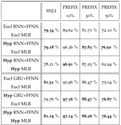
Figure 3 . 5 Test accuracies for various models and four datasets.

“Eucl” denotes Euclidean, “Hyp” denotes hy- perbolic. All word and sentence embeddings have dimension 5 . We highlight in bold the best method (or methods, if the difference is less than 0 . 5 %). Implementation of these experiments was done by co-authors in [GBH

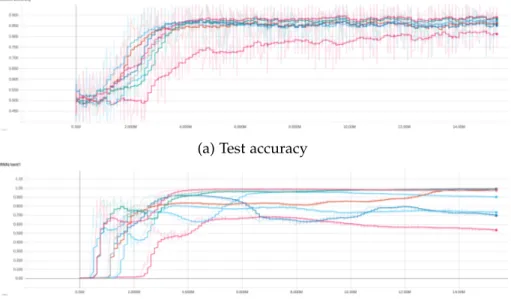
Figure 3 . 6 PREFIX- 30 % accuracy and first (premise) sen-

tence norm plots for different runs of the same

architecture: hyperbolic GRU followed by hy-

perbolic FFNN and hyperbolic/Euclidean (half-

half) MLR. The X axis shows millions of training

examples processed. Implementation of these

experiments was done by co-authors in [GBH

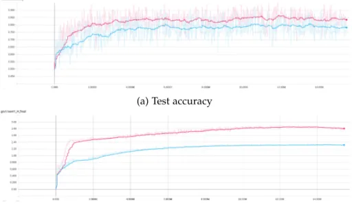
Figure 3 . 7 PREFIX- 30 % accuracy and first (premise) sen- tence norm plots for different runs of the same architecture: Euclidean GRU followed by Eu- clidean FFNN and Euclidean MLR. The X axis shows millions of training examples processed.

Implementation of these experiments was done by co-authors in [GBH

Figure 3 . 8 PREFIX- 30 % accuracy and first (premise) sen-

tence norm plots for different runs of the same architecture: hyperbolic RNN followed by hy- perbolic FFNN and hyperbolic MLR. The X axis shows millions of training examples processed.

Implementation of these experiments was done by co-authors in [GBH

Figure 3 . 9 An example of a hyperbolic hyperplane in

plotted using sampling. The red point is p. The shown normal axis to the hyperplane through p is parallel to a. . . .

Figure 3 . 10 Hyperbolic (left) vs Direct Euclidean (right) bi-

nary

used to classify nodes as being part in the group . n . 01 subtree of the WordNet noun hierarchy solely based on their Poincar´e embed- dings. The positive points (from the subtree) are in red, the negative points (the rest) are in yellow and the trained positive separation hyperplane is depicted in green. . . .

Figure 3 . 11 Test F 1 classification scores (%) for four different

subtrees of WordNet noun tree. 95 % confidence intervals for 3 different runs are shown for each method and each dimension. “Hyp” denotes our hyperbolic MLR, “Eucl” denotes directly apply- ing Euclidean MLR to hyperbolic embeddings in their Euclidean parametrization, and log

de- notes applying Euclidean MLR in the tangent space at

dings there with log

. Implementation of these experiments was done by co-authors in [GBH

Figure 4 . 1 Comparison of the Riemannian and Euclidean

versions of A msgrad . . . .

Figure 4 . 2 Results for methods doing updates with the ex- ponential map. From left to right we report:

training loss, MAP on the train set, MAP on the validation set. . . .

Figure 4 . 3 Results for methods doing updates with the re-

traction. From left to right we report: training loss, MAP on the train set, MAP on the valida- tion set. . . .

Figure 5 . 1 Geodesics in the Poincar´e disk (left) and the

stereographic projection of the sphere (right). . .

Figure 5 . 2 Heatmap of the distance function d

( x, ·) in

for

= − 0.254 (left) and

= 0.248 (right). . . . .

Figure 5 . 3 We illustrate, for a given 2 D point cloud, the

optimal transport plan obtained from minimiz- ing the Wasserstein costs; c (· , ·) denotes the Eu- clidean distance (top) or squared difference (bot- tom). A, B are the Euclidean distance matri- ces obtained from point clouds X, Y. A higher dotted-line thickness illustrates a greater mass transport. . . .

Figure 5 . 4 Left: Spherical gyromidpoint of four points.

Right: M ¨obius gyromidpoint in the Poincar´e model defined by [Ung

] and alternatively, here in eq. (

). . . .

Figure 5 . 5 Weighted Euclidean midpoint

+

. . . .

Figure 5 . 6 Heatmap of the distance from a

-hyperplane

to x ∈

for

= − 0.254 (left) and

= 0.248 (right) . . . .

Figure 5 . 7 Histogram of Curvatures from ”Deviation of

Parallogram Law” . . . .

Figure 5 . 8 Intuition for our Wasserstein prototype model. We

assume that a few prototypes, e.g. some functional

groups, highlight key facets or structural features of

graphs in a particular graph classification/regression

task at hand. We then express graphs by relating

them to these abstract prototypes represented as free

point cloud parameters. Note that we do not learn

the graph structure of the prototypes. . . . .

samples with (right, with weight 0.1) and with- out (left) contrastive regularization for runs using the exact same random seed. Points in the proto- types tend to cluster and collapse more when no regularization is used, implying that the optimal transport plan is no longer uniquely discrimi- native. Prototype 1 (red) is enlarged for clarity:

without regularization (left), it is clumped to- gether, but with regularization (right), it is dis- tributed across the space. . . .

Figure 5 . 10 Left: GNN model; Right: ProtoW-L 2 model;

Comparison of the correlation between graph embedding distances (X axis) and label distances (Y axis) on the ESOL dataset. . . .

Figure 5 . 11 2 D heatmaps of T-SNE [MH

] projections of

molecular embeddings (before the last linear layer) w.r.t. their associated predicted labels.

Heat colors are interpolations based only on the test molecules from each dataset. Comparing (a) vs (b) and (c) vs (d), we can observe a smoother space of our model compared to the GNN base- line as explained in the main text. . . .

L I S T O F TA B L E S

Table 3 . 1 Word similarity results for 100 -dimensional mod- els. Highlighted: the

and the

plementation of these experiments was done in collaboration with co-authors in [TBG

]. . . . .

Table 3 . 2 Nearest neighbors (in terms of Poincar´e dis-

tance) for some words using our 100 D hyperbolic

embedding model. . . .

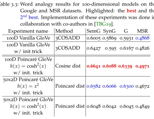
Table 3 . 3 Word analogy results for 100 -dimensional mod- els on the Google and MSR datasets. High- lighted: the

and the

tion of these experiments was done in collabora- tion with co-authors in [TBG

]. . . .

Table 3 . 4 Some words selected from the 100 nearest neigh-

bors and ordered according to the hypernymy score function for a 50 x 2 D hyperbolic embed- ding model using h ( x ) = x

. . . .

Table 3 . 5 WBLESS results in terms of accuracy for 3 dif-

ferent model types ordered according to their difficulty. . . .

Table 3 . 6 Hyperlex results in terms of Spearman correla-

tion for 3 different model types ordered accord- ing to their difficulty. . . .

Table 3 . 7 Average distances,

computed via sampling for the metrics induced by different h functions, as defined in eq. (

).

Table 3 . 8 Similarity results on the unrestricted ( 190 k) vo-

cabulary for various h functions. This table should be read together with Table

. . . .

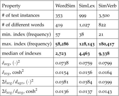
Table 3 . 9 Various properties of similarity benchmark datasets.

The frequency index indicates the rank of a word in the vocabulary in terms of its frequency: a low index describes a frequent word. The median of indexes seems to best discriminate WordSim from SimLex and SimVerb. . . .

Table 5 . 1 Minimum achieved average distortion of the dif-

ferent models.

and

denote hyperbolic and spherical models respectively. . . .

Table 5 . 2 Node classification: Average accuracy across 5

splits with estimated uncertainties at 95 percent

confidence level via bootstrapping on our datas-

plits.

and

denote hyperbolic and spherical

models respectively. Implementation of these

experiments was done in collaboration with co-

authors in [BBG

]. . . .

Table 5 . 3 Average curvature obtained for node classifica- tion.

and

denote hyperbolic and spherical models respectively. Curvature for Pubmed was fixed for the product model. Implementation of these experiments was done in collaboration with co-authors in [BBG

]. . . .

Table 5 . 4 Results of different models on the property pre-

diction datasets. Best in bold, secondbest under- lined. Proto methods are ours. Lower RMSE is better, while higher AUC is better. The prototype- based models generally outperform the GNN, and the Wasserstein models perform better than the model using only simple Euclidean distances, suggesting that the Wasserstein distance pro- vides more powerful representations. Wasser- stein models trained with contrastive regular- ization as described in section

outperform those without. Implementation of these experi- ments was done in collaboration with co-authors in [B´ec+

]. . . .

Table 5 . 5 The Spearman and Pearson correlation coeffi-

cients on the ESOL dataset for the GNN and ProtoW-L2 model w.r.t. the pairwise difference in embedding vectors and labels. Implementa- tion of these experiments was done in collabora- tion with co-authors in [B´ec+

]. . . .

Table 5 . 6 The parameters for our models (the prototype

models all use the same GNN base model), and

the values that we used for hyperparameter

search. When there is only a single value in

the search list, it means we did not search over

this value, and used the specified value for all

models. . . .

ML

Machine Learning

AA

Apprentissage Automatique

CNN

Convolutional Neural Network

GNN

Graph Neural Network

GCN

Graph Convolutional Network

DMPNN

Directed Message Passing Neural Network

OT

Optimal Transport

OTGNN

Optimal Transport Graph Neural Network

SGD

Stochastic Gradient Descent

RSGD

Riemannian Stochastic Gradient Descent

NCE

Noise Contrastive Estimation

FFNN

Feed-forward Neural Network

RNN

Recurrent Neural Network

GRU

Gated Recurrent Unit

MLR

Multinomial Logistic Regression

MDS

Multidimensional Scaling

PCA

Principal Component Analysis

s

1

I N T R O D U C T I O N , M O T I VAT I O N S & G O A L S

1 . 1 a p r i m e r o n m a c h i n e l e a r n i n g

In the last two decades, the combined increased availability of data on the one hand and computational power on the other hand has given rise to a pletora of new powerful statistical methods. Machine Learning grew wider as a field in opposite directions at the same time:

highly engineered, “black box”, uninterpretable models with millions, sometimes billions of parameters partly took over the state-of-the-art spotlight [Bro+

]; [Dev+

]; [KSH

], while most new fundamental contributions were becoming more and more mathematical.

It is worth reminding that what most of these successful models happen to have in common is to either take as input data represented as a Euclidean embedding (be it images, words or waveforms) or to internally represent symbolic data as such. This tendency has naturally motivated the development of general-purpose representations to be used in downstream tasks, the most striking example being perhaps word embeddings with W ord2 V ec [Mik+

lo V e [PSM

] and F ast T ext [Boj+

]. More broadly, finding “good” data representations and understanding what good means has quickly made itself one of the cornerstones of machine learning: Y. Bengio has even described the disentangling of the underlying factors explaining the data as “pre- solving any possible task relevant to the observed data” [Ben

], which has recently been emphasized when a step in this direction won the Best Paper Award at ICML 2019 [Loc+

].

Acknowledging the importance of adequately representing data, we

decided to concentrate our efforts in this direction. The observation of

how relatively unexplored were non-Euclidean geometries in the above

mentionned pipelines, together with a strong taste for geometry, has

led us through the story we tell in this dissertation.

1 . 2 e u c l i d e a n r e p r e s e n tat i o n s 1 . 2 . 1 Power & Ubiquity

As computers allow for significant amounts of operations on num- bers, representing data as finite sequences or grids of numbers quickly appeared as a natural choice. When the necessity to measure similarity or discrepancy between data points came to light, one of the most canonical choices was to generalize to higher dimensions the way we naturally compute distances in our intuition-friendly, 3 -dimensional physical world: via Euclidean Geometry. From a computational stand- point, this geometry has numerous advantages: (i) many important quantities such as distances, inner-products and geodesics can be com- puted very efficiently; (ii) linearity of the Euclidean space provides us with a tremendous amount of mathematical tools, e.g. Linear Algebra or Probability Theory; (iii) reasoning in this space matches in many ways our human intuition, compared to other, more exotic geometries.

Euclidean representations are at the heart of most state-of-the-art models available today, from language modeling [Dev+

]; [Rad+

] to image classification [He+

]; [KSH

], generation [Goo+

], ma- chine translation [BCB

]; [Vas+

], speech recognition [GMH

] or recommender systems [He+

].

1 . 2 . 2 Limitations

Despite its success, as almost any particular model choice, Euclidean Geometry may have certain limitations. Or put another way: non- Euclidean geometries may constitute a superior choice in a given setting.

Indeed, recent research has proven that many types of complex data (e.g. graph data) from a multitude of fields (e.g. Biology, Network Science, Computer Graphics or Computer Vision) exhibit a highly non- Euclidean latent anatomy [Bro+

]. In such cases, where Euclidean properties such as shift-invariance are not desired, the Euclidean space does not provide the most powerful or meaningful geometrical repre- sentations.

Moreover, as canonical as Euclidean Geometry may seem, it actually constraints the geometric properties of certain elementary objects:

1 . The sum of angles of a triangle is always

2 . The volume of a ball grows polynomially with its radius.

3 . Euclidean inner-product defines a positive definite kernel:

∀

∈

\ { 0

} , ∀( x

)

∈ (

)

:

∑

∑

α_iα_j

h x

, x

i > 0.

( 1 . 1 ) which, as one can show (see section

), can be reformulated equivalently as the fact that the squared Euclidean distance de- fines a conditionally negative definite kernel (c.n.d.):

∀

∈

, ∀( x

)

∈ (

)

: if

∑

α_i

= 0, then

∑

∑

α_iα_j

k _x

− _x

k

≤ _{0. (} ¹ _. ² ₎ At this stage, one may wonder: to what extent are these properties restrictive?

Given a task to solve and a discrete/symbolic dataset, there often exists an inherent geometry underlying the task: be it semantic simi- larity in natural language processing or image classification, proximity between users and items in recommender systems, or more broadly:

the geometry that characterizes nearness in the space of labels for any classification or regression problem.

From a given task and dataset, such geometries can be defined by ideal similarity or discrepancy metrics. But, what guarantees that these metrics will share the above listed properties of Euclidean Geometry?

Indeed, there exist other embedding geometries possessing properties contradictory to those listed above. For instance, as we will see in greater details later on, the angles of a triangle sum below (resp. above)

in a hyperbolic (resp. spherical) space. Another example: in a b-ary tree, the number of k-hops neighbors to the root grows exponentially with k; similarly, in a hyperbolic space, the volume of a ball grows exponentially with its radius, which is not the case for Euclidean and spherical spaces. Finally, a Gram matrix need not be positive definite nor c.n.d. to represent a valid similarity or discrepancy kernel.

This immediately raises the question of how can we assess in advance

which geometry is best to embed a dataset, relative to a given task? We discuss

this matter in the next section.

p o n d e r i n g . In practice, additional considerations must be taken into account, than such a geometrical match on a mathematical level:

(i) computational efficiency, of course, but also (ii) hardness of opti- mization. Indeed, the vast majority of embedding methods rely on gradient-based optimization. A non-Euclidean embedding metric could theoretically represent a better choice if one were able to find a good optimum, but may make this optimization problem much harder. De- veloping new non-Euclidean machine learning methods requires to carefully consider these matters.

1 . 3 b e y o n d e u c l i d e a n g e o m e t r y

1 . 3 . 1 Characterizing the Geometry of Discrete Data

As mentionned above, how can we know which embedding geometry would theoretically best suit a given dataset/task? Although this remains an open problem, certain quantities can be computed to get an idea.

m e t r i c d i s t o r s i o n . Given a weighted graph or a discrete metric space, how closely can we embed it into a “continuous” space, so that distances in the latter reflect those in the former? A natural measurement of this distorsion is given by taking the sum, over the finite metric space, of squared differences between the target metric d

and corresponding embeddings x

, x

:

min

∑

i,j

( d ( x

, x

) − d

)

. ( 1 . 3 ) Note that finding a family x of embeddings minimizing distorsion can be intractable in practice. Empirical upper bounds can be obtained either via combinatorial or gradient-based methods (e.g. see [De +

in hyperbolic spaces), and for simple cases theoretical lower bounds can be computed by leveraging the metric properties (e.g. see Section 1 . 3 . 2 of [Gan

]).

δ

- h y p e r b o l i c i t y . This notion, originally proposed by Gromov [Gro

], characterizes how tree-like a space is, by looking at how close is each geodesic segment of a triangle to its barycenter: in a tree, e.g.

for the 3 -star graph made of one root node and four leaf nodes, this

distance is zero; in a Euclidean space, this distance in unbounded; in a hyperbolic space, it is upper bounded by a factor going to zero when curvature goes to −

worst case measure over all triangles in a metric space, more recently Borassi et al. [BCC

] proposed an averaged version yielding more robust and efficiently com- putable statistics for finite graphs. We provide further definitions and explanations about original and averaged

numerical computations, in section

.

d i s c r e t e r i c c i - o l l i v i e r c u r vat u r e . Originally introduced by Y. Ollivier [Oll

], this notion provides a discrete analogue to the celebrated Ricci curvature from Riemannian Geometry. It captures the same intuition: namely, it compares the distance between small balls (w.r.t to optimal transportation) to the distance between their centers: a ratio above (resp. below) one characterizes a positive (resp.

negative) curvature. On a graph, a “ball” and its center are replaced by a (transition) probability distribution over neighbors, allowing to define the curvature of Markov Chains over the graph. It was computed mathematically in expectation for Erd ¨os-Renyi random graphs [LLY

] and empirically for certain graphs representing the internet topology [Ni+

].

Other recent variants exist such as Discrete Foreman [For

] and sectional [Gu+

1 . 3 . 2 Non-Euclidean Properties of Data Embedded in a Euclidean Space

In machine learning and neuroscience, certain computational struc-

tures and algorithms are known to yield disentangled representations

without us understanding why, the most striking examples being per-

haps convolutional neural networks and the ventral stream of the visual

cortex in humans and primates. As for the latter, it was conjectured that

representations may be disentangled by being flattened progressively

and at a local scale [DC

]. An attempt at a formalization of the role of

invariance in learning representations was made recently, being referred

to as I-theory [Ans+

of differential geometry, we will show that pooling over a group of

transformations of the input contracts the metric and reduces its curva-

ture, and provide quantitative bounds, in the aim of moving towards a

theoretical understanding on how to disentangle representations.

1 . 3 . 3 Hyperbolic Representations

Interestingly, [De +

be embedded with arbitrary low distortion (i.e. almost preserving their metric) in the Euclidean space with unbounded number of dimensions, but this task becomes surprisingly easy in the hyperbolic space with only 2 dimensions where the exponential growth of distances matches the exponential growth of nodes with the tree depth.

But how should one generalize deep neural models to non-Euclidean domains? Hyperbolic spaces consitute an interesting non-Euclidean domain to explore for two essential reasons: (i) important mathematical quantities such as distances, exponential map, gradients and geodesics are known in efficiently computable closed-form formulas and (ii) they are known to be better suited than the Euclidean space to represent trees, and hence potentially tree-like graphs as well.

Indeed, the tree-likeness properties of hyperbolic spaces have been extensively studied [Gro

]; [Ham

]; [Ung

] and used to visual- ize large taxonomies [LRP

] or to embed heterogeneous complex networks [Kri+

]. In machine learning, recently, hyperbolic represen- tations greatly outperformed Euclidean embeddings for hierarchical, taxonomic or entailment data [De +

subtrees from the latent hierarchical structure surprisingly disentan- gle and cluster in the embedding space as a simple reflection of the space’s negative curvature. However, appropriate deep learning tools are needed to embed feature data in this space and use it in downstream tasks. For example, implicitly hierarchical sequence data (e.g. textual entailment data, phylogenetic trees of DNA sequences or hierarchial captions of images) would benefit from suitable hyperbolic Recurrent Neural Network (

)s.

On the other hand, Euclidean word embeddings are ubiquitous nowa-

days as first layers in neural network and deep learning models for

natural language processing. They are essential in order to move from

the discrete word space to the continuous space where differentiable

loss functions can be optimized. The popular models of Glove [PSM

],

Word 2 Vec [Mik+

], provide efficient ways to

learn word vectors fully unsupervised from raw text corpora, solely

based on word co-occurrence statistics. These models are then suc-

cessfully applied to word similarity and other downstream tasks and,

surprisingly (or not [Aro+

]), exhibit a linear algebraic structure that is also useful to solve word analogy.

However, unsupervised word embeddings still largely suffer from revealing antisymmetric word relations including the latent hierarchi- cal structure of words. This is currently one of the key limitations in automatic text understanding, e.g. for tasks such as textual entail- ment [Bow+

]. To address this issue, [MC

]; [VM

] propose to move from point embeddings to probability density functions, the simplest being Gaussian or Elliptical distributions. Their intuition is that the variance of such a distribution should encode the generality/specificity of the respective word. However, this method results in losing the arithmetic properties of point embeddings (e.g. for analogy reasoning) and becomes unclear how to properly use them in downstream tasks.

To this end, we propose to take the best from both worlds: we embed words as points in a Cartesian product of hyperbolic spaces and, additionally, explain how they are bijectively mapped to Gaussian embeddings with diagonal covariance matrices, where the hyperbolic distance between two points becomes the Fisher distance between the corresponding probability distribution functions. This allows us to derive a novel principled

on top of word embeddings that can be leveraged for hypernymy detection. We learn these word embeddings unsupervised from raw text by generalizing the Glove method. Moreover, the linear arithmetic property used for solving word analogy has a mathematical grounded correspondence in this new space based on the established notion of parallel transport in Riemannian manifolds.

1 . 3 . 4 Riemannian Optimization

Developing powerful stochastic gradient-based optimization algo- rithms is of major importance for a variety of application domains.

In particular, for computational efficiency, it is common to opt for a first order method, when the number of parameters to be optimized is great enough. Such cases have recently become ubiquitous in engineer- ing and computational sciences, from the optimization of deep neural networks to learning embeddings over large vocabularies.

This new need resulted in the development of empirically very suc-

cessful first order methods such as A dagrad [DHS

], A dadelta

[Zei

], A dam [KB

] or its recent update A msgrad [RKK

].

Note that these algorithms are designed to optimize parameters liv- ing in a Euclidean space

, which has often been considered as the default geometry to be used for continuous variables. However, a recent line of work has been concerned with the optimization of parameters lying on a Riemannian manifold, a more general setting allowing non- Euclidean geometries. This family of algorithms has already found numerous applications, including for instance solving Lyapunov equa- tions [VV

], matrix factorization [Tan+

], geometric programming [SH

], dictionary learning [CS

] or hyperbolic taxonomy embedding [De +

].

A few first order stochastic methods have already been generalized to this setting (see section

), the seminal one being Riemannian Stochastic Gradient Descent (

) [Bon

], along with new methods for their convergence analysis in the geodesically convex case [ZS

].

However, the above mentioned empirically successful adaptive methods, together with their convergence analysis, remain to find their respective Riemannian counterparts.

Indeed, the adaptivity of these algorithms can be thought of as assigning one learning rate per coordinate of the parameter vector.

However, on a Riemannian manifold, one is generally not given an intrinsic coordinate system, rendering meaningless the notions sparsity or coordinate-wise update.

1 . 3 . 5 Graph-like Data

1 . 3 . 5 . 1 On the Success of Euclidean GCNs

Recently, there has been considerable interest in developing learning algorithms for structured data such as graphs. For example, molecular property prediction has many applications in chemistry and drug discovery [Vam+

]; [Yan+

].

Historically, graphs were systematically decomposed into features such as molecular fingerprints, turned into non-parametric graph ker- nels [She+

]; [Vis+

], or, more recently, learned representations via

GNN

[DBV

]; [KW

Indeed, the success of convolutional networks and deep learning for

image data has inspired generalizations for graphs for which sharing

parameters is consistent with the graph geometry. [Bru+

]; [HBL

]

are the pioneers of spectral

in the graph Fourier space using lo-

calized spectral filters on graphs. However, in order to reduce the graph-dependency on the Laplacian eigenmodes, [DBV

mate the convolutional filters using Chebyshev polynomials leveraging a result of [HVG

]. The resulting method is computationally efficient and superior in terms of accuracy and complexity. Further, [KW

simplify this approach by considering first-order approximations ob- taining high scalability. The proposed

locally aggregates node embeddings via a symmetrically normalized adjacency matrix, while this weight sharing can be understood as an efficient diffusion-like regularizer. Recent works extend

s to achieve state of the art results for link prediction [ZC

], graph classification [HYL

]; [Xu+

] and node classification [KBG

]; [Vel+

].

1 . 3 . 5 . 2 Extending GCNs Beyond the Euclidean Domain

In spite of this success, on the one hand, certain types of data (e.g.

hierarchical, scale-free or spherical data) have been shown to be better represented by non-Euclidean geometries [Bro+

]; [Def+

]; [Gu+

[NK

[RS

]; [TDL

] and information geometry [AN

]. The mathematical framework in vigor to manipulate non-Euclidean geometries is known as Riemannian geometry [Spi

]. On the other hand,

are also often underutilized in whole graph prediction tasks such as molecule property prediction. Specifically, while

s produce node embeddings for each atom in the molecule, these are typically aggregated via simple operations such as a sum or average, turning the molecule into a single vector prior to classification or regression. As a result, some of the information naturally extracted by node embeddings may be lost.

These observations led us to (i) propose a first variant of the

architecture, called

, which internally represents data in a family

of chosen non-Euclidean domains, and to propose (ii) another variant,

called Optimal Transport Graph Neural Network (

) dispensing

completely with the final node (sum/average) aggregation yielding the

final Euclidean graph embedding, thus preserving the graph representa-

tion as a point-cloud of node embeddings considered w.r.t. Wasserstein

(Optimal Transport) Geometry.

κ-GCN

. An interesting trade-off between the general framework of Riemannian Geometry, which often yields computationally intractable geometric quantities, and the well-known Euclidean space, is given by manifolds of constant sectional curvature. They define together what are called hyperbolic (negative curvature), elliptic/spherical (positive curva- ture) and Euclidean (zero curvature) geometries. Benefits from rep- resenting certain types of data into hyperbolic [GBH

[NK

] or spherical [Dav+

]; [Def+

]; [Gra+

]; [Gu+

[Mat

]; [Wil+

]; [XD

] spaces have recently been shown. As men- tionned earlier, this mathematical framework has the benefit of yielding efficiently computable geometric quantities of interest, such as distances, gradients, exponential map and geodesics. We propose a unified ar- chitecture for spaces of both (constant) positive and negative sectional curvature by extending the mathematical framework of Gyrovector spaces to positive curvature via Euler’s formula and complex analysis, thus smoothly interpolating between geometries of constant curvatures irrespective of their signs. This is possible when working with the Poincar´e ball and stereographic spherical projection models of respec- tively hyperbolic and spherical spaces.

OTGNN

. As mentionned above, we also seeked to address the potential loss of information incurred by the final node aggregation step present in nearly all

architectures to yield the final graph embedding. As it turns out, recent work by Togninalli et al. [Tog+

] already proposed to dispense with the aggregation step altogether and instead derive a kernel function over graphs by directly comparing node embeddings as point clouds through optimal transport (Wasserstein distance). Their non-parametric model yields better empirical performance over popular graph kernels, but has not been so far extended to the more challenging parametric case. Motivated by this observation and drawing inspiration from prototypical networks [SSZ

], we introduce a new class of

where the key representational step consists of comparing each input

graph to a set of abstract prototypes, as illustrated in Figure

. These

prototypes play the role of dictionary items or basis functions in the

comparison; they are also stored as point clouds as if they were encoded

from actual real graphs. Each input graph is first encoded into a set

of node embeddings using a

. We then compare this resulting

embedding point cloud to those corresponding to the prototypes. For-

mally, the distance between two point clouds is measured by appeal

to optimal transport Wasserstein distances. The prototypes as abstract basis functions can be understood as keys that highlight property val- ues associated with different structural features. In contrast to kernel methods, the prototypes are learned together with the

parame- ters in an end-to-end manner. Our model improves upon traditional aggregation by explicitly tapping into the full set of node embeddings without collapsing them first to a single vector. We theoretically prove that, unlike standard

aggregation, our model defines a class of set functions that is a universal approximator. Most importantly, introduc- ing points clouds as free parameters creates a challenging optimization problem. Indeed, as the models are trained end-to-end, the primary signal is initially available only in aggregate form. If trained as is, the prototypes often collapse to single points, reducing the Wasserstein distance between point clouds into Euclidean comparisons of their means. To counter this effect, we introduce a contrastive regularizer which effectively prevents the model from collapsing (Section

).

We demonstrate empirically that it both improves model performance and generates richer prototypes.

Our contributions are summarized in the following section.

1 . 4 t h e s i s c o n t r i b u t i o n s

This thesis is organized into four chapters, subsequently taking deep dives into manifold representations, methods in hyperbolic spaces, Riemannian adaptive optimization and finally graph-like data.

c h a p t e r 1 . We start by taking interest into the effect of pooling on the geometry of data representations. We prove two theorems about orbit contraction (Theorem

) and flattening (Theorem

), and illustrate the phenomenon of interest via numerical simulations and visualizations.

c h a p t e r 2 . Then, we explore representing data in hyperbolic spaces.

We start by generalizing the word embedding method G lo V e , and de-

scribe how to evaluate similarities and analogies. In particular, leverag-

ing a connection with Fisher information, we develop a new method (Al-

gorithm

) to assess hypernymy, i.e. entailment relationships between

concepts. We motivate the use of hyperbolic geometry by computing

averaged delta-hyperbolicities on a weighted graph obtained from co-

occurence counts, upon which GloVe is based. We then take interest into generalizing neural architectures to hyperbolic spaces, adapting matrix multiplication,

and

, also called softmax. To understand how to perform bias translations, we connect gyro-addition to parallel transport, the latter being computed explicitly (Theorem

) from the Levi-Civita connection and its Christoffel symbols. To adapt

s to hyperbolic spaces, we prove a so-called gyro-chain-rule (Lemma

).

c h a p t e r 3 . Motivated by the lack of hyperbolic analogues to the cel- ebrated Euclidean adaptive optimization algorithms (A dam , A dagrad , A ms G rad ) − much needed for high performance of various embedding methods, including the training of G lo V e − we study adapting those to certain Riemannian manifolds (Algorithm

guarentees (Theorems

and

), recovering the known bounds in the particular case of Euclidean spaces. Our methods are validated on the task of embedding the WordNet hierarchy in the Poincar´e Disk.

c h a p t e r 4 . Finally, we investigate leveraging non-Euclidean geome-

tries to better represent graph-like data. We start by adapting

to

hyperbolic and spherical spaces by leveraging Einstein midpoint opera-

tions (Definition

) and explore certain of its mathematical properties

(Theorems

-

-

), showing good empirical performance on graph

embeddings (w.r.t. distorsion) and node classification. In a second part,

we take interest into dispensing with the final aggregation step per-

formed by most

architecture. We do so by computing Wasserstein

distances (Optimal Transport) between point-clouds of node embed-

dings and so-called prototype point-clouds, i.e. free parameters. We

study properties of universality (Theorem

) and non-definiteness

(Theorem

) of the resulting kernel and introduce a new regularizer

(Eq. (

)) inspired from Noise Contrastive Estimation (

), whose

use we show is crucial in order to prevent the model from naturally

collapsing back to the standard sum/average node aggregation. We

illustrate the empirical efficacy of the method with both qualitative and

quantitative experiments on molecular datasets.

2

G R O U P I N VA R I A N C E & C U RVAT U R E O F R E P R E S E N TAT I O N S

What does disentangling representations mean? In machine learning and neurosciences, representations being tangled has two principal interpretations, and they are intimately connected with each other. The first one is geometrical: consider two sheets of paper of different colors, place one of the two on top of the other, and crumple them together in a paper ball; now, it may look difficult to separate the two sheets with a third one: they are tangled, one color sheet representing one class of a classification problem. The second one is analytical: consider a dataset being parametrized by a set of coordinates { x

}

, such as images parametrized by pixels, and a classification task between two classes of images. On the one hand, we cannot find a subset { x

}

with J ⊂ I of this coordinate system such that a variation of these would not change the class of an element, while still spanning a reasonable amount of different images of this class. On the other hand, we are likely to be capable of finding a large amount of transformations preserving the class of any image of the dataset, without being expressible as linear transformations on this coordinate system, and this is another way to interpret representations or factors of variation as being tangled.

Why is disentangling representations important? On the physiologi- cal side, the brains of humans and primates alike have been observed to solve object recognition tasks by progressively disentangling their representations via the visual stream, from V 1 to the IT cortex [DC

];

[DZR

]. On the side of deep learning, deep convolutional neural networks are also able to disentangle highly tangled representations, since a softmax − which, geometrically, performs essentially a linear separation − computed on the representation of their last hidden layer can yield very good accuracy [KSH

]. Conversely, disentangling repre- sentations might be sufficient to pre-solve practically any task relevant to the observed data [Ben

].

How can we design algorithms in order to move towards more disen-

tangled representations? Although it was conjectured that the visual

stream might disentangle representations by flattening them locally,

thus inducing a decrease in the curvature globally [DC

], the mecha- nisms underlying such a disentanglement, whether it be for the brain or deep learning architectures, remain very poorly understood [Ben

];

[DC

]. However, it is now of common belief that computing represen- tations that are invariant with respect to irrelevant transformations of the input data can help. Indeed, on the one hand, deep convolutional networks have been noticed to naturally learn more invariant features with deeper layers [Goo+

]; [LV

]; [TM

]. On the other hand, the V 1 part of the brain similarly achieves invariance to translations and rotations via a “pinwheels” structure, which can be seen as a prin- cipal fiber bundle [Pet

]; [Pog+

]. Conversely, enforcing a higher degree of invariance with respect to not only translations, but also rotations, flips, and other groups of transformation has been shown to achieve state-of-the-art results in various machine learning tasks [BM

]; [CW

]; [CW

]; [DDK

]; [GD

]; [OM

], and is believed to help in linearizing small diffeomorphisms [Mal

]. To the best of our knowledge, the main theoretical efforts in this direction include the theory of scattering operators [Mal

]; [WB

] as well as I-theory [Ans+

]; [ARP

]. In particular, I-theory permits to use the whole apparatus of kernel theory to build invariant features [MVP

]; [Raj+

].

Our work builds a bridge between the idea that disentangling is a result of (i) a local decrease in the curvature of the representations, and (ii) building representations that are invariant to nuisance deformations, by proving that pooling over such groups of transformations results in a local decreasing of the curvature.

We start by providing some background material, after which we introduce our formal framework and theorems, which we then discuss in the case of the non-commutative group generated by translations and rotations.

Research presented in this chapter was conducted at the very begin- ning of the author’s PhD, and was only published as an ArXiv preprint [B´ec

].

2 . 1 b a c k g r o u n d m at e r i a l

2 . 1 . 1 Groups, Lie Algebras & Haar Measures

A group is a set G together with a map · _: G × G → G such that: