WITCHING R EGRESSION A PPROACH F RONTIER OF S OUTHERN M EXICO :A S L AND U SES IN AN A GRICULTURAL S EMI -S UBSISTENT AND C OMMERCIAL M ODELING THE D ETERMINANTS OF

10.1177/0160017604266029INTERNATIONAL REGIONAL SCIENCE REVIEW (Vol. 27, No. 3, 2004) ARTICLE

Vance, Geoghegan / MODELING THE DETERMINANTS OF LAND USES

M ODELING THE D ETERMINANTS OF

S EMI -S UBSISTENT AND C OMMERCIAL

L ^AND U ^{SES IN AN} A GRICULTURAL

F RONTIER OF S OUTHERN M EXICO : A S ^WITCHING R ^EGRESSION A ^PPROACH

COLINVANCE

German Aerospace Center, Institute of Transport Research, Berlin, Germany, colin.vance@dlr.de

JACQUELINEGEOGHEGAN

Department of Economics, Clark University, Worcester, MA, jgeoghegan@clarku.edu

The authors analyze the consequences of imperfect output markets for the land-use decisions of semi-subsistence farmers in an agricultural frontier of southern Mexico. The approach is moti- vated by previous applications of the agriculture household model establishing that the farm household’s production and consumptiondecisions are analytically nonseparable when markets are not used. Econometric results generated by a switching regression model suggest the impor- tance of distinguishingthe discrete choice of market participationfrom that of area cultivated.

Keywords: agricultural household models; separable models; switching regression

Tropical deforestation is significant to a range of themes that have relevance for the study of environmental change and economic development, including global warming, land degradation, species extinction, and sustainability issues. Recogni- tion that both thelocationandpatternof forest clearance are often as important as itsmagnitudehas motivated an increasing number of empirical studies aimed at modeling the spatial dimensions of deforestation processes (e.g., Chomitz and Gray 1996; Nelson and Hellerstein 1997; Cropper, Griffiths, and Mani 1999; Pfaff 1999). A majority of these studies assume that agents are fully engaged in markets and therefore that their production behavior can be empirically specified using a profit-maximizing framework. However, as much tropical deforestation occurs in developing countries in areas often characterized by underdeveloped markets, the assumption of full market participation by land managers is tenuous at best. Conse- quently, the results from these models may be biased, implying that policies derived therefrom may be misinformed. In this article, we draw on the example of an

DOI: 10.1177/0160017604266029

© 2004 Sage Publications

agricultural frontier from southern Mexico to analyze the land-use decisions of farmers operating in a context of thin markets. Our focus abstracts from the defor- estation process per se to address the agricultural land uses that result in land clear- ance, as it is this underlying behavior that can be influenced through conservation programs. Applying lessons from a growing body of studies in the agricultural development literature (e.g., Huang, Raunikar, and Misra 1991; Goetz 1992;

Sadoulet, de Janvry, and Benjamin 1998; Key, Sadoulet, and de Janvry 2000), we suggest that modeling land-use decisions necessitates distinguishing the discrete choice of participation in agricultural product markets from the continuous choice of area cultivated. Accordingly, our empirical approach advances the existing liter- ature on land-use modeling by employing a switching regression that partitions households according to their participation in output markets while simultaneously controlling for biases emerging from sample selectivity.

R

P

L

Although some of the spatial deforestation models show divergences in empiri- cal results according to the commercial versus semi-subsistence agricultural land- use distinction, the maintained modeling assumption for both land-use types is of profit maximization. For example, using the profit-maximizing framework, Chomitz and Gray (1996) for Belize and Cropper, Griffiths, and Mani (1999) for Thailand showed that the effect of roads on deforestation levels tend to be greater for commercial crops.¹These studies also identified the effect of soil quality on deforestation to differ by the market orientation of the crop grown. However, as these authors only had available aggregate socioeconomic data, they imposed the commercial versus semi-subsistence designation; in Chomitz and Gray, this was done by crop type; and in Cropper, Griffiths, and Mani, it was inferred by geographical region.

Similarly, previous household-level models of land use in developing regions do not directly question the validity of the profit-maximization framework, but the evi- dence from many studies suggests that the framework may not be appropriate for understanding land-use choices. For example, Jones et al. (1995) discovered possi- ble evidence of the divergence between profit and utility maximization in several

This work was undertaken through the auspices of the Southern Yucatán Peninsular Region project with core sponsorship from NASA’s LCLUC (Land-Cover and Land-Use Change) program (NAG 56406) and the Center for Integrated Studies on Global Change, Carnegie Mellon University (CIS-CMU; NSF- SBR 95-21914).Additional funding from NASA’s New Investigator Program in Earth Sciences (NAG5- 8559) also supported the specific research in this article. This project is a collaborative project of El Colegio de la Frontera Sur (ECOSUR), Harvard Forest–Harvard University, the George Perkins Marsh Institute–Clark University and CIS-CMU. We would like to thank all of our project colleagues, espe- cially Peter Klepeis, Yelena Ogneva-Himmelberger, Rinku Roy Chowdhury, and Laura Schneider for their help with the survey and satellite data. We would also like to thank Kathleen Bell and Julie Hewitt for very helpful comments. The views expressed in this article are those of the authors and are not neces- sarily the official views of the Environmental Protection Agency.

subsistence crops among farmers in Brazil. Monela (1995), Godoy et al. (1997), and Pichón (1997) identified demographic effects on deforestation in Tanzania, Honduras, and Ecuador, respectively, which should not be the case under profit maximization.

While it is generally recognized that the existence or absence of markets is pro- foundly linked to the land allocation decision (Godoy et al. 1997; Omamo 1998a, 1998b), there has been little research on this linkage in frontier regions where mar- kets for goods and factors remain underdeveloped or missing. With few exceptions, spatial microeconomic models of deforestation assume a full and complete set of markets, thereby justifying the analysis of the farm household’s production deci- sions in isolation from its consumption decisions. At the same time, there exists a long-standing recognition within the agricultural development literature that such an analytical division is often inappropriate in regions with underdeveloped mar- kets. This recognition has stimulated the development agricultural household mod- els that explicitly incorporate the interdependency of the household’s production and consumption decisions on the allocation of household resources (e.g., Wharton 1969; Barnum and Squire 1979; Singh, Squire, and Strauss 1986). Given the ability of these models to explain the sometimes sluggish—and even perverse—response of peasants to changes in relative prices, this approach represents a potentially important analytical tool for assessing the effects of price-based policy measures in curtailing deforestation.

B

R

In this article, we draw on a spatially explicit data set from a sample of Mexican farm households to test the implications of using the agricultural household model for land-use choices. Our research focuses specifically on theejidosector of Mexi- can agriculture as this is currently the predominate form of land tenure in the study region. This sector was created following the Mexican Revolution (1910-17), a political and social upheaval with roots in inequitable land distribution. Within ejido communities, land is communally regulated by an elected committee, but in this area of southern Mexico, ejido members(ejidatarios)typically enjoy usufruct access to a single parcel that is permanently allocated to their use.²This tie between households and parcels permits land-use decisions to be linked to the geographical locations in which they have impact.

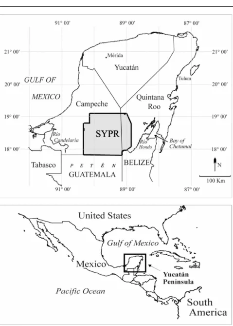
The study region, located in the southern portion of the Yucatán peninsula (see Figure 1), is part of the largest continuous expanse of tropical forests remaining in Central America and Mexico and has been identified as a “hot spot” of forest and biotic diversity loss (Achard et al. 1998). For the first half of the twentieth century, economic activity here was minimal and centered on the selective logging of tropi- cal woods, particularly mahogany and cedar, as well as on the extraction of chicle, a tree resin used in the production of chewing gum. More extensive deforestation fol- lowed with the construction of a two-lane highway paved east-west across the cen-

ter of the region in 1967, which opened the frontier to agricultural colonization via the extension ofejidalland grants, as sanctioned by Article 27 of the Mexican con- stitution.³

Most early settlers of the region arrived in the mid 1970s from neighboring regions of Mexico where there was a scarcity of land. They practiced predomi-

FIGURE 1. The Southern Yucatán Peninsular Region (SYPR)

nantly subsistence-oriented systems of land-use management as exemplified by the milpa, a centuries-old form of Maya agriculture dominated by maize and typically intercropped with beans and squash (Turner 1983). In recent years, however, there has been a trend toward land-use diversification that features the expansion of cash crop production, most notably the cultivation of chili peppers. Based on the accounts of various respondents, chili peppers seem to have first appeared in the region in the late 1970s. In contrast to maize, which is grown primarily for subsis- tence but a portion of which is occasionally sold, the entire output of chili peppers is marketed. This distinction affords an opportunity to explore whether a different economic behavior underlies the production of these two crops. We have available individual household survey data, including information on demographics, crop choices, the area planted, and if the crops were sold, that allow us to examine the implications of incomplete markets in the spatial modeling of agricultural expan- sion leading to tropical deforestation.

T

C

Two broad classes of the agricultural household model have been developed to explain differing production strategies of farm households depending on market opportunities (Singh, Squire, and Strauss 1986). The first class of models, called theseparable model, exists when all input, output, and insurance markets fully function. These conditions make it optimal for the utility-maximizing farmer to apply a production logic that is independent of consumption considerations. With prices for factors of production and output exogenously given, utility and profit- maximizing production calculations converge. Such models are sometimes referred to asrecursivebecause there is a one-way effect of the optimizing produc- tion decision on consumption via the level of income obtained. Empirically, this implies that an econometric specification based on profit-maximization is suffi- cient to model the farmer’s allocation of factors of production.

The second class of models isnonseparable, where the consistency of utility and profit-maximizing behavior no longer holds. This can occur when the transaction costs of market exchange are sufficiently high to induce the household to opt for self-sufficiency, as may result, for example, from prohibitively costly transport due to poor infrastructure connecting farms with regional market centers (Omamo 1998a, 1998b). When the household chooses not to participate in the market, its production and consumption decisions cannot be analytically separated: produc- tion decisions will incorporate subsistence and/or leisure considerations. Empiri- cally, this implies that a profit-maximizing specification comprising only prices and technology will yield biased estimates. Correcting this bias necessitates incor- porating variables that also measure the consumption side of household decision making.

Two types of transaction costs—fixedandproportional—may result in the deci- sion not to participate in the market (Key, Sadoulet, and de Janvry 2000). Fixed

transaction costs are invariant to the quantity of the good traded and include search, bargaining, and labor supervision costs. Proportional transaction costs, by contrast, vary with the extent of market participation and typically arise from the per-unit costs of trading in markets and imperfect information. Both types of cost lead to a low farm gate price at which farmers can sell their crop and a higher price at which they can buy that crop at the market. Figure 2 illustrates this circumstance for the case of proportional transaction costs, with the exogenously given price band Pbuy

and Psell(de Janvry, Sadoulet, and Gordillo de Anda 1995).

There are three market participation choices for a household depending on the position of their supply curve and demand curve relative to the price band. Self- sufficiency will occur if the intersection of these curves falls within the price band.

In this case, the household’s endogenous valuation of maize (i.e., the shadow price) is lower than the price it would pay were it to purchase maize in the market but higher than the price it would receive were it to sell maize. As the equilibrium price is no longer parametric, but rather is determined endogenously by the choices of the household, production of this nontraded good is directly linked to its consumption.

Therefore, the household will allocate that amount of land to maize that ensures the equilibrium of its marginal cost and marginal benefit schedules, implying that the food consumption requirement will affect production decisions. For a household with a relatively high marginal cost of production, the shadow price will be above the market purchase price and the household will purchase in the market the quan- tityab. Conversely, for a low-marginal-cost household, the equilibrium is below the lower limit, and they will sell the quantitycd. In either of these instances, the food consumption requirement is expected to have no effect on the production decision.

Price

Quantity Demand

P_buy P_sell Supply of high marginal cost producer: purchases maize

Supply of low marginal cost producer: sells maize

Supply of mid marginal cost producer: self-sufficient

c

a b

d

FIGURE 2. Illustrating Separability

Several theoretical and empirical studies have applied the above framework to focus on the implications of missing or thin markets for labor (Lopez 1986;

Benjamin 1992; Jacoby 1993; Sadoulet, de Janvry, and Benjamin 1998), food (de Janvry, Fafchamps, and Sadoulet 1991; Goetz 1992; Omamo 1998a, 1998b), and insurance (Roe and Graham-Tomasi 1986; Saha 1994).⁴A fundamental result emerging from this body of literature is that if a complete set of markets exists, the optimal land-use portfolio is one that equalizes the marginal revenue product of the land across all uses. Since this outcome is a function of exogenously given market parameters and is independent of household characteristics, measures of demo- graphic composition should have no statistically significant effect in explaining land use for households that participate in all markets, even if these households consume a portion of their output. This observation is the basis for the empirical tests pursued in this article. Drawing on the framework provided by the agricultural household model, hypotheses are formulated that relate demographic structure to both semi-subsistence and commercially based land-use choices under different market participant regimes.

T

S

D

Q

Selection of respondents for the household survey proceeded according to a stratified, two-stage cluster sample (Warwick and Luinger 1975; Deaton 1997), with ejidos as the first-stage unit and ejidatarios as the second-stage unit. Using maps and population censuses published by the Mexican government’s national institute of statistics and geography (INEGI 1985-87, 1991a, 1991b), the region was partitioned into eleven geographic strata, and one ejido (orcluster) was ran- domly selected from each of the strata. Each ejido was assigned a probability of selection equal to the ratio of its population to the population of the stratum. In the second stage, the survey respondents were randomly selected, whereby the target number of households surveyed from each ejido was approximated such that the corresponding stratum was represented in roughly the same proportion as its share of the total population of the study zone. In the empirical analysis that follows, the data were weighted to adjust for deviations from this target.

A standardized questionnaire, administered to the household head, was used to elicit the socioeconomic and land-use data. The first section covered migration his- tory, farm production and inputs, off-farm employment participation, and the demographic composition of the household. Completion of the second section involved a guided tour of the agricultural plot of the respondent. Using a global positioning system (GPS), the interviewer created a geo-referenced sketch map detailing the configuration of land uses, including the area allocated to commercial and subsistence crops. In combination with available satellite imagery, topographic maps published by INEGI (1985-87), and rainfall data, this information was entered into a geographic information system (GIS), thereby enabling the calcula- tion of spatially explicit indices such as distance to road and ecological measures.

E

S

Two econometric models are specified, the first for maize, which is cultivated by the entire sample, but is sold by slightly less than half; and the second for chili pep- pers, which is only cultivated by approximately half of the sample, but is produced strictly for the market. Both models use a form of the two-stage switching regres- sion model to test hypotheses concerning which parameters are statistically signifi- cant in explaining land-use choices in an environment of potentially imperfect mar- kets. Our approach follows an empirical methodology originally formulated by Lee (1982) and used by Goetz (1992) to study marketed surplus of food grains in Sene- gal conditional on market participation. Variants of the methodology were subse- quently applied by Sadoulet, de Janvry, and Benjamin (1998) and by Key, Sadoulet, and de Janvry (2000) in studies from Mexico of labor market participation and agri- cultural household supply response, respectively. In this article, we apply the gen- eral version of the switching regression to study maize cultivation. A special case of the technique, Heckman’s (1974) sample selection model, is applied to chili cultivation as in that case the dependent variable is censored at zero.

The theoretical framework outlined above indicated that the determinants of maize cultivation are contingent on the decision of the household to participate as a seller in the market. As the decision to sell maize is itself an endogenous choice, however, there may be unobservable variables that affect both the probability of being a seller as well as the area of maize planted. To account for the potential simultaneity bias arising from the existence of such variables, the empirical specifi- cation employs a two-stage, switching regression model with endogenous switch- ing (Lee 1982; Maddala 1983).

The model considers that observations are ordered into two regimes. In the context of the present example, these regimes correspond to the area allocated to maize cultivation among the sellers and nonsellers, represented by the following equations:

Regime 1 (sellers):yi=β′₁X_1i+u_1iifτ′Zi≥ui (1) Regime 2 (nonsellers):yi=β′₂X_2i+u_2iifτ′Zi<ui. (2) In this system, theXiare the exogenous determinants of area cultivated, theZiare the determinants of seller status, and theβ′andτ′are vectors of the associated pa- rameters to be estimated. The error termuiis assumed to be correlated with the er- rors u_1i and u_2i, and all three terms are assumed to have a trivariate normal distribution.

The first stage defines a dichotomous variable indicating the regime into which the observation falls:

Si= 1 ifτ′Zi≥uI

Si= 0 otherwise. (3)

After estimating the parametersτusing the probit maximum likelihood method, the expected values of the residuals,ui, are calculated. As theuiare normally distrib- uted, with meanσ_1uuiand varianceσ₁²–σ_1u², these values are given by the standard formula for the expected value of a truncated distribution (Greene 1997):

E(u_1i|ui≤ τ′Zi) =E(σ_1uui|ui≤ τ′Zi) = –σ_1u[ϕ(τ′Zi)/φ(τ′Zi)] (5) E(u_2i|ui≥ τ′Zi) =E(σ_2uui|ui≥ τ′Zi) =σ_2u[ϕ(τ′Zi)/(1 –φ(τ′Zi))]. (6) The bracketed terms on the right hand side of equations 5 and 6 of the above equa- tions represent two variants of the inverse Mills ratio, defined by the ratio of the density function of the standard normal distribution,ϕ, to its cumulative density function,φ. When appended as an extra regressor in the second-stage estimation, this ratio is a control for potential biases arising from sample selectivity. Denoting the two variants of the inverse Mills ratio asw₁andw₂, the second-stage regressions can then be written as

y_seller=β′₁X_1i–σ_1u[w₁] +ε_1iifτ′Zi≥ui (7) y_nonseller=β′₂X_2i–σ_2u[w₂] +ε_2iifτ′Zi<ui, (8) where the estimated coefficients—σ_1uandσ_2u—give covariance estimates of the unobserved effects on the selling and planting decisions (Killingsworth 1983). If significant, these estimates indicate that sample selectivity is present. Because the residuals of the second-stage regressions are heteroskedastic, they are estimated by weighted least squares using the Huber/White estimates of variance.

As in the case of maize, the problem of estimating the area cultivated in chili peppers needs to distinguish between the determinants of market participation and those of area cultivated. The decision to produce chili simultaneously represents a decision to participate in the market as the entire output is sold, but because 48 per- cent of the sample produced no chili whatsoever, a modified version of the switch- ing regression, the Heckman sample selection model, is used. The model considers that there is an index, si*, that determines whether the observation yi(the area allocated to chili pepper cultivation) is observed:

si* =τ′Zi+ui,si= 1 ifsi* > 0 and 0 otherwise, and yi=β′xi+εiobserved whensi= 1.

(9) (10)

Under the assumption thatuiandεiare jointly normally distributed, the expected value ofyican be written by inserting the inverse Mills ratio, as in equation 5:

E[yi|yiis observed] =β′xi+E[εi|ui<τ′Zi] =β′xi+ρ[ϕ(τ′Zi)/φ(τ′Zi)], (11) whereρrepresents the correlation betweenuiandεi. The model, which comprises an equation determining sample selection and a regression model, can be estimated using the maximum likelihood technique, with estimates of the inverse Mills ratio used as starting values in the iteration process.

M

I

C

V

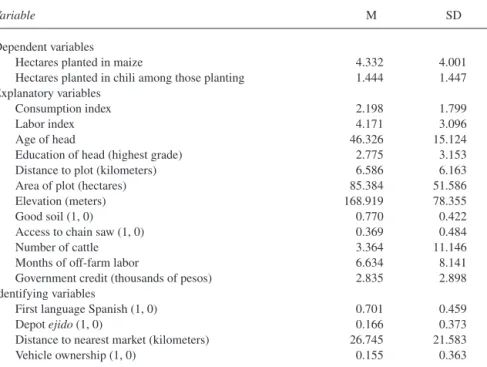
To identify both empirical models requires the selection of variables that uniquely determine the discrete decision (e.g., whether to participate in the market) but not the continuous decision (e.g., area cultivated). In the present example, this selection can be informed by the work of Goetz (1992) and of Key, Sadoulet, and de Janvry (2000), where these authors demonstrated that the market participation decision depends on both fixed and proportional transaction costs while the extent of participation depends on proportional transaction costs only. Identification of the model can therefore be achieved by including in the selector equation variables that proxy for fixed transaction costs. We include five such variables: a dummy variable for vehicle ownership, the on-road distance from the ejido to the nearest market and its square, a dummy variable indicating one of the sampled ejidos that is situated on the main highway and serves as a depot for local produce, and a dummy variable indicating whether the head of the household is a native Spanish speaker.⁵ The descriptive statistic for these and the other variables of the model are presented in Table 1. Following the work of Goetz, the identifying variables are intended to control for the fixed costs of information gathering and of accessing the market. We expect that the dummies for vehicle ownership, the favorably situated ejido, and first language in Spanish positively affect the probability of market participation as they reduce information and access costs. Conversely, distance is predicted to have a negative effect, with the squared term included to allow for potential nonlinearities.

Among the other exogenous regressors presented in Table 1 are variables theo- retically expected to affect the continuous land-use decision: demographic indices, travel costs to the plot, time allocated to off-farm labor, available liquidity, farm capital (human and physical), and ecological factors. With regard to the demo- graphic indices, we hypothesize that the sellers of maize and chili, having made the decision to participate in the market, will reach their production decision for each of these two crops with reference to the associated farm-gate prices. Consequently,

there should be no statistically significant relationship between area of maize or chili planted and the consumption requirement of the household. Such a relation- ship, however, is expected among households producing maize solely for subsis- tence. As their valuation of that crop is determined endogenously as a function of demographic composition, we expect to observe a positive effect of the household consumption requirement on the area of maize cultivated.⁶

To distinguish between household supply of labor and consumption demand effects, demographic structure is decomposed into two mutually exclusive vari- ables that were constructed on the basis of educational attainment and age. The first variable measures the number of household members greater than or equal to twelve years of age who have less than nine years of schooling and is intended to measure the potential pool of domestic on-farm labor (Sadoulet, de Janvry, and Benjamin 1998).⁷The second variable, comprising children under twelve and members with nine or more years of schooling, measures the remainder of the household. Since young children and highly educated members are assumed to not contribute to field labor, this variable is taken to be a consumption measure that is purged of an on-farm supply-side effect.⁸No a priori prediction is made for the

TABLE 1. Descriptive Statistics of Variables Used in the Regressions

Variable M SD

Dependent variables

Hectares planted in maize 4.332 4.001

Hectares planted in chili among those planting 1.444 1.447 Explanatory variables

Consumption index 2.198 1.799

Labor index 4.171 3.096

Age of head 46.326 15.124

Education of head (highest grade) 2.775 3.153

Distance to plot (kilometers) 6.586 6.163

Area of plot (hectares) 85.384 51.586

Elevation (meters) 168.919 78.355

Good soil (1, 0) 0.770 0.422

Access to chain saw (1, 0) 0.369 0.484

Number of cattle 3.364 11.146

Months of off-farm labor 6.634 8.141

Government credit (thousands of pesos) 2.835 2.898

Identifying variables

First language Spanish (1, 0) 0.701 0.459

Depotejido(1, 0) 0.166 0.373

Distance to nearest market (kilometers) 26.745 21.583

Vehicle ownership (1, 0) 0.155 0.363

coefficient on the household labor force measure other than to exclude a negative sign. Given the existence of thin labor markets, the measure would be expected to have a positive coefficient, reflecting nonseparability in production and con- sumption as a consequence of the household’s endogenous valuation of its time endowment.

Aside from the consumption index defined above, we have no theoretical basis for expecting differential effects of the remaining control variables according to whether the crop is sold. The travel cost of plot access, measured by the walking distance from the household, is expected to reduce the area planted as it detracts from labor hours available for cultivation and also effectively reduces the farm-gate price received for the crop. Likewise, to the extent that off-farm employment diverts household labor away from cultivation and may additionally relax pressures to gen- erate cash and food from farm activities, this measure is also expected to have a nega- tive effect on area cultivated for maize and chili (Godoy et al. 1997; Pichón 1997).

To control for available liquidity, the total aid in government credit received since 1996 and the number of cattle owned are included. While credit may be directed to land-improving investments (e.g., fertilizer) that reduce the area culti- vated, it may also be directed to labor-saving investments (e.g., tractors) that increase area cultivated. Hence, the net effects are unclear. The effects of cattle are also ambig- uous. In the case of a poor harvest, cattle can either be sold or consumed to supple- ment staple requirements, an insurance mechanism that could be expected to increase the extent of commercialized nonfood crops such as chili peppers. Cattle also may have, however, a negative effect across maize and chili since large tracts are required for grazing, thereby reducing the area available for other land uses.

Three variables control for the effects of ecological factors: the total land endowment, a dummy variable indicating favorable soil quality, and the average elevation of the plot. The total land endowment is expected to have a positive coeffi- cient since, all else equal, greater access to land promotes more extensive (and labor-saving) farming practices. With regard to expectations on the remaining vari- ables, we simply note that while more favorable ecological conditions would increase the probability that a given plot is cultivated, it is not possible to predict their effect on the actual size of the plot.

The education and age of the household head and a dummy for access to a chain- saw are included as measures of available human and physical farm capital. More education not only may enhance labor productivity through increased managerial talent and the adoption of modern farm technologies (Godoy et al. 1997; Tao Yang 1997) but also implies a higher opportunity cost of on-farm labor due to increased wage earning potential. Hence, it is expected to exert a negative effect on the area cultivated. Similar effects of managerial talent could be expected for the age of the household head. The effects of access to a chainsaw are hypothesized to be positive through lowering of the labor costs in forest clearance.

E

R

Results from the first-stage probit analysis used to identify the determinants of seller status are presented in Table 2. Turning first to the identifying variables, it is seen that the signs on most of the coefficient estimates are consistent with intuition.

The dummy variables indicating the favorably situated ejido and vehicle ownership are both positive, likely reflecting the lower costs of information gathering and increased accessibility. The other measure of information-gathering costs, the Spanish language dummy, unexpectedly has a negative and significant coefficient.

This finding may be a consequence of cultural attributes that make Mayan farmers, from whose ancestors the milpa system of maize cultivation evolved, more likely to

TABLE 2. Probit and Weighted Least Squares (WLS) Models of Seller Status and Hectares Planted in Maize

WLS of Hectares Planted in Maize

Variable Probit of Seller Status Sellers Nonsellers

Consumption index –0.030 (–0.357) –0.443 (–0.732) 1.134 (3.447)***

Labor index –0.041 (–1.822) 0.257 (2.086)* 0.384 (2.914)**

Age of head –0.002 (–0.256) 0.055 (2.347)* 0.004 (0.157)

Education of head –0.466 (–1.144) 0.168 (1.137) –0.051 (–0.542) Distance to plot 0.024 (1.678) –0.101 (–1.729) –0.078 (–4.044)***

Area of plot 0.004 (3.109)** 0.002 (0.229) 0.011 (1.650)

Elevation 0.002 (1.831) –0.007 (–1.208) –0.002 (–0.550)

Good soil –0.163 (–0.480) 1.938 (2.336)* 0.777 (1.978)*

Access to chainsaw –0.030 (–0.171) 0.107 (0.088) –0.527 (–0.665) Number of cattle –0.015 (–1.902)* –0.026 (–0.987) 0.057 (0.860) Months of off-farm labor 0.005 (0.753) 0.180 (1.909)* –0.067 (–0.865) Government credit 0.061 (2.642)** 0.530 (2.510)** 0.332 (2.857)**

First language Spanish –0.548 (–2.134)**

Depotejido 1.212 (1.985)*

Distance to nearest market 0.074 (2.524)**

Distance squared –0.001 (–2.045)*

Vehicle ownership 0.504 (2.812)**

Selectivity term (sell = 1) 0.447 (0.273)

Selectivity term (sell = 0) –2.274 (–2.612)**

Constant –2.210 (–2.565)* –0.352 (0.19) 1.394 (0.92)

R² .45 .37

Observations 187 78 109

Note: T-statistics appear in parentheses.

*Significant at the 10% level. **Significant at the 5% level. ***Significant at the 1% level.

sell that crop. Distance to market has a nonlinear effect on the probability of seller status, first increasing and then decreasing.

The signs on most of the remaining variables are also consistent with intuition.

Access to credit and a larger land endowment positively affect the probability of seller status, with the latter result likely due to the fact that with more land, farmers are able to extend the fallow period, thereby increasing the land’s productivity for future use in the cycle. Cattle ownership decreases the probability of seller status, which is probably a consequence of pasture creation removing land from the maize fallow cycle. Finally, the labor endowment and the distance from the household to the plot are statistically insignificant.

S^TAGE2: T^HEDETERMINANTS OFA^REACULTIVATED INM^AIZE

With the inverse Mills ratio included as a regressor to control for selectivity bias, the next two models in Table 2 test hypotheses concerning the determinants of maize cultivation for the sellers and nonsellers of that crop, respectively. Sample selectivity appears to be an issue only in the nonseller regression, with the negative coefficient on the inverse Mills ratio likely reflecting the influence of unobservable variables that lead a nonseller to plant less maize than a household selected at ran- dom (Goetz 1992). The most noteworthy distinction revealed by the model is the asymmetric effect of the consumption index. This variable is significant in the nonseller regression while it is insignificant among the sellers, thereby lending sup- port to the hypothesis that the latter regime reaches their production decision inde- pendent of consumption considerations.⁹

Other than the consumption index, however, there are few variables that suggest a distinctly different behavior between the two regimes. Consistent with intuition, the dummy variable indicating favorable soil and the credit index are positive and significant in both models. Likewise, the labor index is also seen to be positive and significant in the two models. Although in this case we had no a priori predictions, this finding likely reflects the household’s endogenous valuation of its own labor due to some combination of limited opportunities for off-farm employment, lim- ited availability of labor for hire, and potentially higher monitoring costs associated with hired labor. Differential effects are seen with respect to the variables measur- ing the total family months allocated to nonfarm labor in the previous year, the age of the household head, and the distance separating the household from its agricul- tural plot. The former two are positive and significant for the sellers only, while the latter is negative and of roughly the same magnitude for both groups but significant for the nonsellers only.

C^HILIP^EPPERS

The final model investigates the determinants of commercial chili pepper pro- duction with an application of Heckman’s sample selection model. To allow for

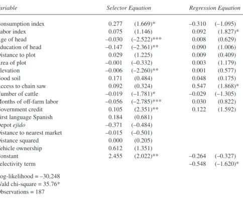
qualitative comparisons, the specification includes the same variables in the selec- tor and regression equations that were used in the model for maize. The results pre- sented in Table 3 suggest that the many of the factors determining both the partici- pation and production decisions for chili are different from those of maize.

Included among the statistically significant determinants of the market participa- tion decision for chili are the consumption index, the age and education of the household head, months allocated to off-farm labor, and the elevation of the plot, none of which were significant determinants of the market participation decision for maize. The remaining two statistically significant variables, cattle ownership and credit, are also significant for the case of maize and of the same sign. Overall, it appears that the household’s pool of available labor, as captured by the demo- graphic indices and by the months allocated to off-farm labor, is an important factor in determining the decision to enter the chili market. This finding may relate to the fact that the harvest for chili occurs over a highly concentrated time span during which the family must harness its entire stock of labor, both skilled and unskilled.

Those households heavily committed to the off-farm labor market may thus be

TABLE 3. Heckman Model of Producer Status and Hectares Planted in Chili Peppers

Variable Selector Equation Regression Equation

Consumption index 0.277 (1.669)* –0.310 (–1.095)

Labor index 0.075 (1.146) 0.092 (1.827)*

Age of head –0.030 (–2.522)*** 0.008 (0.629)

Education of head –0.147 (–2.361)** 0.090 (1.006)

Distance to plot 0.029 (1.225) 0.009 (0.409)

Area of plot –0.001 (–0.332) 0.003 (1.179)

Elevation –0.006 (–2.260)** 0.001 (0.577)

Good soil 0.171 (0.484) 0.048 (0.175)

Access to chain saw 0.092 (0.324) 0.547 (1.868)*

Number of cattle –0.019 (–1.781)* –0.029 (–1.305)

Months of off-farm labor –0.056 (–2.785)*** 0.030 (0.822)

Government credit 0.105 (2.351)** 0.122 (1.592)

First language Spanish 0.184 (0.681)

Depotejido –0.371 (–0.484)

Distance to nearest market –0.015 (–0.501)

Distance squared 0.000 (0.205)

Vehicle ownership 0.612 (1.351)

Constant 2.455 (2.022)** –0.264 (–0.327)

Selectivity term –0.548 (–1.620)*

Log-likelihood = –30,248 Wald chi-square = 35.76*

Observations = 187

Note: Z-statistics appear in parentheses.

*Significant at the 10% level. **Significant at the 5% level. ***Significant at the 1% level.

deterred from planting chili. It is also notable that the coefficient on distance to mar- ket and its square are statistically insignificant. This may result from differences in the marketing networks of maize and chili. Whereas maize is generally transported by the farmers themselves, chili is transported by marketing intermediaries locally referred to ascoyoteswho typically purchase the harvest at or near the site of the farmer’s field. While none of the identifying variables are individually significant, the overall appropriateness of the selector equation specification is supported by a significant estimate for the sample selection parameter.

Turning to the regression results, only two variables are seen to be statistically significant in explaining the area planted in chili: the labor index and ownership of a chainsaw, the former of which was also significant for the case of maize. Consistent with expectation that the household’s valuation of chili is determined exogenously by the market price, the consumption index has no statistically significant effect in determining the area cultivated. That the chainsaw dummy is positive and signifi- cant, contrasting with the case of maize, underscores the reports of many farmers to only clear plots having mature trees for planting chili.

M

E

P

I

The above models have demonstrated that households facing idiosyncratic dif- ferences in the transaction costs of market participation will exhibit differences in production behavior according to seller status. Returning to the land-use and defor- estation policy question raised in the introduction, it is of interest to move beyond assessing the statistical significance of the coefficient estimates to also consider their magnitude. To this end, we focus on two variables that potentially could serve as policy tools, credit and travel distance to the farm plot, both of which were identi- fied as significant determinants of maize cultivation. Specifically, we wish to com- pare our results to those based on a framework that ignores the possibility that households are differentially integrated into product markets, as is the common approach in the land-use literature.

We begin by noting that when the exogenous variables of interest appear in both the selector equation and regression equations of the switching regression model, there are a number of alternative approaches to calculating their associated mar- ginal effects (Maddala 1983; Dolton and Makepeace 1987; Huang, Raunikar, and Misra 1991; Goetz 1992). One approach is to simply refer to the coefficient esti- mate of the regression equation itself. This estimate has been euphemistically referred to in the literature as the potential or “desired” effect, though whatever eco- nomic content such an interpretation carries generally receives little elaboration.

More relevant interpretations are derivable by calculation of what are called the conditionaland unconditional marginal effects. The former is calculated sepa- rately for each regime, using information conditional on the observation being in that regime. As such, this estimate is used when the objective of the analysis is to understand decision making for a specific subset of observations while adjusting

for selectivity biases. Conversely, the unconditional marginal effect is calculated based on information from the entire sample and is appropriate when the objective is to assess the effect of an exogenous variable irrespective of the regime. This effect can further be decomposed into a quantity response from those already in one of the two regimes and an adjustment factor for selectivity bias resulting from entry or exit from the regimes (McDonald and Moffitt 1980; Huang, Raunikar, and Misra 1991).

We examine these different interpretations by focusing on maize, as this is the crop that virtually all farmers in the region cultivate but that less than half choose to sell. With respect to the two policy variables noted above, Table 4 compares the coefficient estimates from an identically specified “straw man” ordinary least squares (OLS) regression that pools the sellers and nonsellers with the potential, conditional, and unconditional marginal effect calculations from the switching regression model. While comparison of the OLS and conditional coefficients reveal only minor differences, more substantial discrepancies emerge with refer- ence to the unconditional effects. This is particularly the case with the travel dis- tance to plot measure, which undergoes a counterintuitive sign shift for the seller regime. The source of this shift is revealed by the decomposition of effects into quantity and selectivity adjustment components. The selectivity adjustment is posi- tive and of higher absolute magnitude than the quantity response, which retains the intuitive negative sign. The unconditional marginal effect for the sellers thus sug- gests that increased travel distance unexpectedly increases the area in maize culti- vated. To the extent that travel distance proxies for the farm-gate price received by the household, this result may reflect the perverse supply response that is often said to characterize farm systems in the intermediate stages of market integration (e.g., Medellin, Apedaile, and Pachico 1994). Therefore, from a policy perspective, it is quite possible that measures to reduce travel costs (e.g., road building) will elicit outcomes that are not predicted by models predicated on the assumption of profit- maximizing farm households. While there is not the dramatic sign shift for the credit variable, the magnitudes are different, leading to different predictions of the responsiveness of farmers to exogenous changes in government credit availability.

C

The empirical results presented in this article highlight the analytical advantages of distinguishing the determinants of land-use decisions according to the house- hold’s relationship with the market. By controlling for the endogeneity of the mar- ket participation decision and subsequently estimating separate regressions by seller status, the switching regression model revealed a number of differences in land-use determinants that otherwise would not have been detected. Moreover, the methodology permitted these effects to be assessed in terms of both conditional and unconditional effects.

TABLE 4.Comparing Marginal Effects Conditional EffectsUnconditional Effects = Quantity Response + Selectivity Adjustment Ordinary Least Squares VariableRegression: Entire SampleSellersa Nonsellersb Sellersc Nonseller Distance to plot–.075–.083–.087.014 = –.036 + .050–.077 = –.050 + Government credit.507.577.308.319 = .189 + .130.143 = .214 + a.E(y1|S= 1)/∂x=β1+τσ1u[(τ′Zi)w1+w12 ]. b.E(y2|S= 0)/∂x=β2–τσ2u[(τ′Zi)w2–w22 ]. c.E(y1)/∂x=β1φ(.) +τϕ(.)[β′1X1i+ (τ′Zi)σ1u]. d.E(y2)/∂x=β2[1 –φ(.)] –τϕ(.)[β′2X2i+ (τ′Zi)σ2u].

343

The most general finding of the article is that the agricultural household’s relationship with the market is important for explaining how it reaches both semi- subsistence and commercial land-use decisions. In the case of the semi-subsistence crop, maize, the significance of the consumption index was argued to be a result of market imperfections for output; while in the case of the commercial crop, chili, the consumption index was, as predicted, an insignificant determinant of area culti- vated. In both the models of maize and chili, the household’s labor endowment was positive and significant, likely reflecting the existence of thin markets for labor.

While the findings presented here address the land uses that displace forests rather than the clearance process itself, they do have important implications for for- est conservation policies. Most important, they suggest that policy instruments that rely on market-based parameters may not have the intended effect in influencing peasant land-use choices if they are not complemented by policies that also reduce the transaction costs of market participation. The reason, as illustrated by the nonseparable agricultural household model, is the prohibitive transaction costs that restrict peasants in their responses to market incentives and constrain them to reach their production decisions with reference to household-specific supply and demand conditions. In this regard, this study complements the existing literature that focuses on forest clearance by illuminating the underlying behavioral incentives and constraints of frontier land managers, which in turn suggests a reexamination of some well-established empirical findings.

The positive effect of roads on deforestation, for example, has almost exclu- sively been analyzed as a consequence of profit-maximizing behavior. Building new roads is said to exacerbate the rate of deforestation by making access to remote, forested areas less costly, thereby increasing the farm-gate price received for agricultural outputs and the resulting returns to clearing lands for agricultural use. This effect, however, may be more a story of migration than one of locational rents defined by profits from production. The road subsidizes the costs of encroach- ment and clearance, regardless of whether this is in response to subsistence or mar- ket incentives. While the outcome, deforestation, may be the same, the behavior that results in this outcome is not, and this has important implications for policy over the longer run once initial access is established. If the decision rules that drive land-use change are primarily subsistence-based, then standard policy measures to influence the rate of this change may have a muted or unintended effect that could not be predicted by the profit-maximizing framework.

In a broader sense, this research has demonstrated that the conditions on which the separable model rests for its validity—profit-maximizing agents operating in competitive markets—may be too stringent for the conditions that typically prevail in agricultural frontiers. This is not to argue for the complete rejection of the separa- ble model but rather to suggest that deforestation should not necessarily be ana- lyzed as a consequence of profit-maximizing behavior for the purpose of policy formulation. Robust models of land-use change necessitate theoretical and empiri- cal approaches that are sensitive to the local market conditions faced by land man-

agers. This sensitivity can be achieved through a careful scrutiny of whether exist- ing market constraints, if there are any, require the use of a nonseparable framework to understand land-use decision making.

N

1. Cropper, Griffiths and Mani (1999) used a measure of road density to capture the effect of roads. In this regard, the authors identify their model as nonspatial (p. 60), in contrast to the spatial model of Chomitz and Gray (1996), which includes a measure of distance to road. However, in both cases, the authors are controlling for the spatial issue of market access.

2. Roughly 7 percent of households had access to multiple, noncontiguous plots. In the majority of these cases, cultivation occurred on only one of these plots for the year of questioning.

3. Article 27 was promulgated following the peasant-led revolutionof 1910and sanctionedthe return of lands that had been appropriated by large haciendas to peasant communities. In 1992, reforms were enacted that terminated the continued extension ofejidalland grants. In addition, the reforms gave ejidatariosthe right to rent or sell their land and to enter into business arrangements with outside inves- tors, all of which were prohibited under the original terms of Article 27. While the long-run conse- quences of these reforms are potentially profound, research by Klepeis (2000) suggests that they have had minimal impact on smallholder farmers in the region to date.

4. Of these studies, Omamo’s (1998a, 1998b) are the only ones that investigate implications for land use, focusing on the relationship between the transaction costs of market participation and the mix of commercial and staple crops.

5. Thirty-one percent of household heads spoke an indigenous language, usually of Mayan origin, as their native language.

6. Strictly speaking, the separable model predicts the insignificance of demographic variables on maize cultivation for both the seller and buyer categories of households. While 26 percent of the house- holds in the sample reported themselves to have occasionally purchased maize for the survey year, the analysis merges these households with the self-sufficient producers under the assumption that the two categories apply an identical operating logic to the productive resources available. Maize cultivation is the principal occupation of most household heads, particularly among the buyers. As a result, we assume that any purchases of maize were more likely to be the result of unexpected shortages relative to domestic consumption rather than of planned production targets.

7. In a study of labor markets in Mexico’sejidatariosector, these authors present persuasive theoreti- cal and empirical evidence to support the proposition that skilled labor (defined by nine or more years of schooling) only works in off-farm employment.

8. Following Pichón (1997), children were weighted by one-third to approximate their consumption requirement relative to adults.

9. One caveat regarding this finding is that no distinction was made between the ex ante decision of how much maize to plant and the ex post decision of how much to sell. The latter decision is partly deter- mined by the quantity of realized output, an amount the farmer cannot be sure of at the time of planting.

Hence, the observance of market participation ex post is not a sufficient condition for the specification of a non-recursive (i.e., profit-maximizing) model, since ex ante the farmer may still be reaching his deci- sion on the basis of the consumption requirements of the household. A high level of risk aversion could exacerbate this problem by leading households to plant an area far larger than that required to feed the family in an average year, thereby increasing the likelihood that they have a surplus for sale. One empiri- cal implication of this feature is that the seller category may consist partly of households that are reach- ing their decisions with reference to consumption considerations, which would increase the chance of falsely rejecting separability for this group.

R

Achard, F., H. Eva, A. Glinni, P. Mayaux, T. Richards, and H. Stibig, eds. 1998.Identification of defores- tation hot spot areas in the humid tropics. Trees Publ. Series B. Research Report no. 4. Brussels:

Space Application Institute, Global Vegetation Monitoring Unit. Joint Research Centre, European Commission.

Barnum,H., and L. Squire.1979.A model of an agricultural household. Washington,DC: WorldBank.

Benjamin, D. 1992. Household composition, labor markets, and labor demand: Testing for separation in agricultural household models.Econometrica60: 287-322.

Chomitz, K. M., and D. A. Gray. 1996. Roads, land, markets and deforestation: A spatial model of land use in Belize.World Bank Economic Review10: 487-512.

Cropper, M., C. Griffiths, and M. Mani. 1999. Roads, population pressures, and deforestation in Thai- land, 1976-1989.Land Economics75: 58-73.

de Janvry, A., M. Fafchamps, and E. Sadoulet. 1991. Peasant household behavior with missing markets:

Some paradoxes explained.Economic Journal101: 1400-1417.

de Janvry, A., E. Sadoulet, and G. Gordillo de Anda. 1995. NAFTA and Mexico’s maize producers.

World Development23: 1349-62.

Deaton, A. 1997.The analysis of household surveys: A microeconomic approach to development policy.

Baltimore: Johns Hopkins University Press.

Dolton, P. J., and G. H. Makepeace. 1987. Interpreting sample selection effects.Economic Letters24:

373-79.

Godoy, R., J. Franks, K. O’Neill, S. Groff, P. Kostishack, A. Cubas, J. Demmer, K. McSweeney, J. Over- man. D. Wilkie, N. Brokaw, and M. Martínez. 1997. Household determinants of deforestation by Amerindians in Bolivia.World Development25: 977-87.

Goetz, S. J. 1992. A selectivity model of household food marketing behaviour in Sub-Saharan Africa.

American Journal of Agricultural Economics74: 444-52.

Greene, W. H. 1997.Econometric analysis. 3rd ed. Upper Saddle River, NJ: Prentice Hall.

Heckman, J. J. 1974. Shadow prices, market wages, and labor supply.Econometrica42: 679-94.

Huang, C., R. Raunikar, and S. Misra. 1991. The application and economic interpretation of selectivity models.American Journal of Agricultural Economics73: 496-501.

INEGI. 1985-87.Cartas topograficas. 1:50,000. Aguascalientes, Mexico: Instituto Nacional de Estadistica Geografica e Informatica.

. 1991a.Campeche: XI Censo General de Poblacion y Vivienda.Resultados Definitivos, Datos por Localidad Aguascalientes.Aguascalientes, Mexico: Instituto Nacional de Estadistica Geo- grafica e Informatica.

. 1991b.Quintana Roo: XI Censo General de Poblacion y Vivienda.Resultados Definitivos, Datos por Localidad Aguascalientes.Aguascalientes, Mexico: Instituto Nacional de Estadistica Geografica e Informatica.

Jacoby, H. G. 1993. Shadow wages and peasant family labour supply: An econometric application to the Peruvian Sierra.Review of Economic Studies60: 903-21.

Jones, W. D., V. H. Dale, J. J. Beauchamp, M. A. Pedlowski, and R. V. O’Neill. 1995. Farming in Rondonia.Resource and Energy Economics17: 155-88.

Key, N., E. Sadoulet, and A. de Janvry. 2000. Transaction costs and agricultural household response.

American Journal of Agricultural Economics82: 245-59.

Killingsworth, M. R. 1983.Labor supply. New York: Cambridge University Press.

Klepeis, P. 2000. Deforesting the once deforested: Land transformation in southeastern México. Doc- toral diss., Graduate School of Geography, Clark University, Worcester, MA.

Lee, L. F. 1982. Some approaches to the correction of selectivity bias.Review of Economic Studies49:

355-72.

Lopez, R. E. 1986. Structural models of the farm household that allow for interdependent utility and profit-maximization decisions. InAgricultural household models: Extensions, applications, and policy, ed. I. Singh, L. Squire, and J. Strauss. Baltimore: Johns Hopkins University Press.

McDonald, J., and R. Moffitt. 1980. The uses of Tobit analysis.Review of Economics and Statistics60:

318-21.

Maddala, G. S. 1983.Limited-dependent and qualitative variables in econometrics. Cambridge: Cam- bridge University Press.

Medellin, M., L. Apedaile, and D. Pachico. 1994. Commercialization and price response of a bean- growing farming system in Columbia.Economic Development and Cultural Change23: 795-816.

Monela, G. C. 1995. Tropical rainforest deforestation, biodiversity benefits, and sustainable land use:

Analysis of economic and ecological aspects related to the Nguru Mountains, Tanzania. Doctoral diss., Agricultural University of Norway, Aas.

Nelson, G. A., and D. Hellerstein. 1997. Do roads cause deforestation? Using satellite images in econo- metric analysis of land use.American Journal of Agricultural Economics79: 80-88.

Omamo, S. W. 1998a. Farm-to-market transaction costs and specialisation in small-scale agriculture:

Explorations with a non-separable household model.Journal of Development Studies35: 152-63.

. 1998b. Transport costs and smallholder cropping choices: An application to Siaya District, Kenya.American Journal of Agricultural Economics80: 116-23.

Pfaff, A. 1999. What drives deforestation in the Brazilian Amazon? Evidence from satellite and socio- economic data.Journal of Environmental Economics and Management37: 26-43.

Pichón, F. J. 1997. Colonist land-allocation decisions, land use, and deforestation in the Ecuadorian Amazon frontier.Economic Development and Cultural Change44: 127-64.

Roe, T., and T. Graham-Tomasi. 1986. Yield risk in a dynamic model of the agricultural household. In Agricultural household models: Extensions, applications, and policy, ed. I. Singh, L. Squire, and J.

Strauss. Baltimore: Johns Hopkins University Press.

Sadoulet, E., A. de Janvry, and C. Benjamin. 1998. Household behavior with imperfect labor markets.

Industrial Relations37: 85-108.

Saha, A. 1994. A two-season agricultural household model of output and price uncertainty.Journal of Development Economics45: 245-69.

Singh, I., L. Squire, and J. Strauss, eds. 1986.Agricultural household models: Extensions, applications, and policy. Baltimore: Johns Hopkins University Press.

Tao Yang, Dennis. 1997. Education and off-farm work.Economic Development and Cultural Change 45: 613-32.

Turner, B. L., II. 1983.Once beneath the forest: Prehistoric terracing in the Rio Bec region of the Maya lowlands. Dellplain Latin American Studies no. 13. Boulder, CO: Westview.

Warwick, D. P., and C. A. Luinger. 1975.The sample survey: Theory and practice. New York: McGraw- Hill.

Wharton, C., Jr., ed. 1969.Subsistence agriculture and economic development. Chicago: Aldine.