Measuring the electron mass through Compton scattering
Data analysis 2021 – Group project II
Vadym Denysenko, Patrick Owen ,Olaf Steinkamp April 13, 2021
1 Motivation
In this project, you simulate an experiment to determine the electron mass using Comp- ton scattering.
Compton scattering, the inelastic scattering of a photon on a charged particle (usually an electron), is named after Arthur Holly Compton who first described this process in 1923. In the scattering process, some of the energy of the photon is transfered to the recoiling charged particle, i.e. the energy of the photon decreases and its wavelength increases. Compton derived the following relation between the wavelength λin of the incoming photon, the wavelength λout of the outgoing photon and the angleθ by which the photon is scattered:
λout−λin = h
mec(1−cosθ) ,
whereh is Planck’s constant, cis the speed of light and me is the mass of the electron.
It is easy to rewrite this equation in terms of the energyEin of the incoming photon and the energy Eout of the outgoing photon:
Eout Ein
= 1
1 + mcEin2 (1−cosθ).
MeasuringEout as a function of cosθ for knownEin will allow to determine me . An important cross check in simulation studies is the so-called “pull”, defined as
pull = reconstructed quantity−generated quantity uncertainty on reconstructed quantity ,
Source
Detector
θ
Ei
Ef
Figure 1: Setup of the experiment.
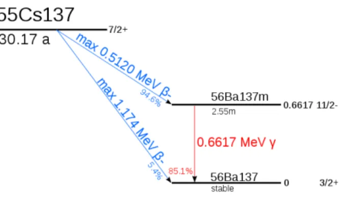
Figure 2: Decay scheme of 137Cs (source: Wikipedia).
where the “uncertainty on reconstructed quantity” is for example that returned from your fit to the data. If the reconstruction is unbiased and the uncertainties on the reconstructed quantities is estimated correctly, the distribution of the pull over many simulated experiments should follow a Gaussian distribution with µ = 0 and σ = 1. If µdeviates significantly from zero, the measurement is biased. Ifσ deviates significantly from one, the uncertainties are not estimated correctly.
2 Setup
A sketch of the setup is shown in Figure 1. It consists of a radioactive source emitting photons of a known energyEin, a thin target in which these photons scatter on electrons, and a moveable detector to measure the final energy Eout of the photons at various scattering anglesθ.
The source contains 137Cs, a radioisotope of Cesium that decays to 137Ba by β decay, i.e. by emitting an electron; with about 95% probability, the137Ba is produced in an ex- cited state, which decays to the stable ground state by emitting a photon with an energy of 0.6617 MeV. The decay scheme is illustrated in Figure2. The source is embedded in
2
a protective shielding with only a small hole through which photons can escape. The in- coming direction of the photons can be assumed to be known with negligible uncertainty and the scattering angle is given by the position of the detector.
In case you wonder, the electronvolt (eV) is a unit of energy used in nuclear and particle physics: 1 eV corresponds to the amount of energy that is gained by a particle with charge e when it is moved across a potential ∆V = 1 V.
3 Simulate the experiment
First, simulate one measurement:
(a) Using the known mass of the electron and the known incoming energy of the photons, calculate the expected outgoing energy Eouttrue(θi) of the photon for θi = 10,20,30. . .80◦. Simulate the finite energy resolution of the photon detector by adding to each Eouttrue(θi) a different random value ∆Ei, drawn from a Gaussian distribution with mean µ= 0 and standard deviationσE = 0.01 MeV. This gives you a measured energy Eoutreco(θi) = Eouttrue(θi) + ∆Ei for each θi. Plot your data points.
(b) Perform a maximum likelihood fit to your set of simulated data pointsEoutreco(θi) to determine the measured electron mass,mrecoe , and its uncertainty. Plot the result of your fit together with your data points.
4 Estimate the uncertainty of the experiment
Now simulate many measurements to check that the uncertainty returned by your fit makes sense:
(a) Repeat the simulation 1’000 times (each time with a new set of ∆E values, always drawn from a Gaussian distribution with mean µ = 0 and standard deviation σE = 0.01 MeV).
(b) Produce a histogram with the 1’000 values of mrecoe that you obtained. Determine the standard deviation of the distribution.
(c) Produce a histogram with the pull distribution formrecoe . Determine the mean and the standard deviation of the pull distribution.
Finally, check how the uncertainty on the electron mass depends on the energy resolution of your detector:
(a) Repeat the exercise for different values of the assumed energy resolution of your detector, i.e. change the standard deviation of the Gaussian from which you draw your ∆E values, first to σE = 0.05 MeV and then to σE = 0.1 MeV.
3