Test of pulse shape analysis using single Compton scattering events

Regular Article – Experimental Physics

Test of pulse shape analysis using single Compton scattering events

I. Abt, A. Caldwell, K. Kr¨ oninger

, J. Liu, X. Liu

, B. Majorovits

Received: 10 October 2007 / Revised version: 29 January 2008 /

Published online: 27 February 2008−© Springer-Verlag / Societ`a Italiana di Fisica 2008

Abstract. Procedures developed to separate single- and multiple-site events in germanium detector are tested with specially selected event samples provided by an 18-fold segmented prototype germanium detec- tor for phase II of the germanium detector array, GERDA. The single Compton scattering, i.e. single-site, events are tagged by coincidently detecting the scattered photon with a second detector positioned at a de- fined angle. A neural network is trained to separate such events from events which come from multi-site dominated samples. Identification efficiencies of≈80% are achieved for both single- and multi-site events.

PACS.23.40.-s; 14.60Pq; 29.40.-n

1 Introduction

Photons of energies around 2 MeV have a high probabil- ity to interact in germanium through Compton scattering.

The mean free path of the process is

4.6 cm. If a photon Compton scatters only once inside a germanium detector, the recoiling electron deposits its energy most likely within a 1 mm range, resulting in a so-called single-site event (SSE). If, in contrast, a photon interacts through pair pro- duction or scatters multiple times, energy can be deposited at different locations separated by typically a few centime- ters, resulting in a so-called multi-site event (MSE). The charge carriers created by the energy deposition in the ger- manium detector drift towards the anode and cathode of the detector. While the charge amplitude of the induced pulse is determined by the number of carriers (thus by the energy deposited), the time spectrum of the pulse (pulse shape) is determined by the location(s) of the energy de- position(s) and thus the charge drifting times. MSEs are expected to have more involved pulse shapes than SSEs, and thus, pulse shape analysis (PSA) can be used to sepa- rate the two classes of events [1–6].

One application of PSA is the background rejection in experiments searching for neutrinoless double-beta decay (0νββ) in

Ge-enriched detectors, such as the GERDA experiment [7]. The expected 0νββ signal events have two electrons in the final state with a total energy of 2.039 MeV.

These are mostly SSEs. A large fraction of the expected background events are induced by external photons with energy depositions around the Q-value. These events are

a Current address: II. Physikalisches Institut, Universit¨at G¨ottingen, Germany

b e-mail: xliu@mppmu.mpg.de

expected to be predominantly MSEs which can be rejected by PSA.

In order to study and improve the performance of PSA, SSE- and MSE-dominant data samples have to be collected independently of the pulse shape. In this paper a method to collect single Compton scattering events (SCS) as an SSE- dominant sample is investigated in more detail. The energy of the scattered photon in an SCS event can be calcu- lated given the incoming photon energy and the scattering angle. Therefore, SCS events can be collected by position- ing a second germanium detector at a specific angle with respect to the first detector and using it to tag escaped photons with the correct energy [2]. If the incoming pho- ton has an energy of 2.614 MeV as emmitted by a

Tl source, a photon Compton scattered at 72

has an energy of 575 keV. This signature is used to tag the single recoiling electron inside the first germanium detector. The energy in the event is equal to the germanium 0νββ Q-value. The lo- cation of the energy deposition of the electron within the detector volume is controlled by positioning the source and the second detector correspondingly.

Another common method to collect an SSE-dominant sample is to select the double-escape events (DEP) [1, 3, 4, 6]. The incoming photon interacts with the germanium detector through pair production and the two 511 keV photons from the positron annihilation escape the detector without further interaction. The electron and positron mostly deposit their energies very locally and re- sult in an SSE. Another useful sample contains so-called single-escape events (SEP) where only one 511 keV photon escapes. The other photon mostly deposits its energy at lo- cations different from those of the electron and positron.

Thus, SEP events provide an MSE-dominant sample with

energy deposition close to the 0νββ Q-value.

426 I. Abt et al.: Test of pulse shape analysis using single Compton scattering events

However, the DEP events are not a perfect test sample for the expected 0νββ events. If the two photons escape the detector, the interaction point is more likely close to the de- tector surface as compared to SCS events. 0νββ events, on the other hand, are distributed evenly within the detector volume. In addition, DEP and 0νββ events have different energies. A DEP event induced by a 2.6 MeV photon from a

Tl source has an energy of 1.59 MeV, quite different from the 0νββ Q-value. In these respects studies with SCS samples suffer less from systematic effects.

The experimental setup and the data collection are de- scribed in Sect. 2. The Monte Carlo simulation is also in- cluded in this chapter. It is used to verify that the collected SCS samples are SSE-dominated. In Sect. 3 a PSA package based on an artificial neural network (ANN) is presented.

The training methods are described and the results given.

2 Experimental setup, data selection and MC simulation

2.1 Experimental setup

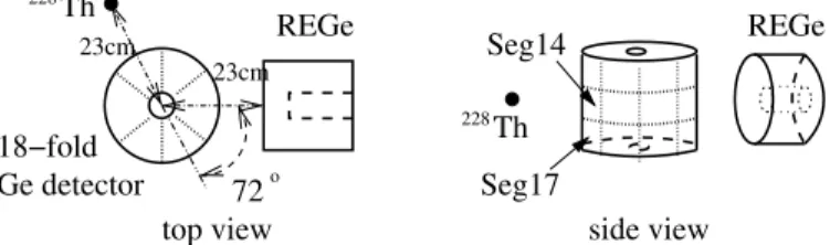
The experimental setup is illustrated in Fig. 1. The seg- mented germanium detector under study is a prototype detector for Phase-II of the GERDA experiment [7]. The true coaxial 18-fold segmented n-type HPGe dectector has a weight of 1.63 kg and the dimensions are 69.8 mm height and 75.0 mm diameter; the inner hole has a diameter of 10.0 mm. The segmentation scheme is 3-fold along the ver- tical axis and 6-fold in the azimuthal angle (see Fig. 1).

Signals from the 18 segments and the core of the detec- tor are amplified by charge sensitive pre-amplifiers and read out by a Pixie4 DAQ system [9] with 14-bit ADC’s at a sampling rate of 75 MHz. The resolution (FWHM) of the core is

3.5 keV at 1.3 MeV and those of the segments are between 2.5 and 4.0 keV. A time resolution of roughly 10 ns can be achieved with the sampling rate used. This corresponds to a position resolution of

1 mm inside the detector volume.

More information about the segmented detector and the DAQ system can be found in [10].

A 100 kBq

Th source is positioned at a distance of 23

1 cm from the center of the segmented detector and faces the center point of segment 14, as illustrated in Fig. 1.

A second non-segmented and well-type germanium detec- tor, a Canberra reversed germanium detector (REGe) [11], is positioned at the same height with the closed end fac- ing the segmented germanium detector. The distance from the closed end surface to the center of the segmented de- tector is 23

1 cm. The REGe crystal is 60 mm in height and 65 mm in diameter. It has a resolution (FWHM) of 2.3 keV at 1.3 MeV. It is used to tag the photons scat- tered mostly in segment 14. The geometrical acceptance of the REGe detector results in recorded SCS events with scattering angles between

65

and

80

corresponding to energy depositions in the segmented detector between

1 The typical drift velocity of the charge carriers inside a ger- manium detector is≈1 cm per 100 ns.

Fig. 1. Schematic of the experimental setup with the 18-fold segmented germanium detector as target and the REGe de- tector to tag photons at 72^◦ (not to scale). The dotted lines illustrate the segment boundaries

≈

1940 keV and

2110 keV. The precision of the alignment of the REGe detector with respect to the

Th source and the segmented detector is

5

.

The energy thresholds for all channels are set to 100 keV. A coincidence trigger is required between the core of the segmented detector and the REGe with a coinci- dent time window of 500 ns. Due to a technical limitation of the coincidence trigger of the DAQ system, only four channels could be read out. Thus, for each coincidence trigger, only the energies of the core (E

), segment 14 (E

), segment 17 (E

) (below segment 14, as illus- trated in Fig. 1) and the REGe (E

) were recorded. 300 time samples were taken for each pulse for all 4 channels.

This corresponds to a time window of 4

before the arrival of the trigger. In this analysis, however, only the core pulses are used for the PSA.

The actual coincidence trigger rate was

12 Hz. The independent trigger rates of the segmented detector and of the REGe detector were both

2000 Hz. This results in an accidental coincidence rate of

2 Hz. The coincidence trig- ger rate without the

Th source is

0.1 Hz. Therefore, without further cuts,

20% of all events are expected to originate from accidental coincidences.

However, the frac- tion of accidental coincidence events among the selected SCS events is negligible, as discussed in the next section.

2.2 Event selection

In total 360 000 coincident events were collected. Four dif- ferent data samples are selected:

–

: single-Compton-scattering (SCS) events

|ECore

+

2614.5

5.0 keV

and

1940

2090 keV

583.2

3.0 keV

–

: events with the 2.6 MeV photon fully absorbed in the segmented detector

|ECore−

2614.5

5.0 keV –

: DEP events

|E_Core−

1592.5

5.0 keV (two 511 keV photons escape.) –

: SEP events

|ECore−

2103.5

5.0 keV (one 511 keV photon escapes).

The

sample is selected through three cuts. The allowed window of

5 keV of the sum energy of both detec-

2 The fraction is expected to differ for different energy ranges, as the trigger rate varies.

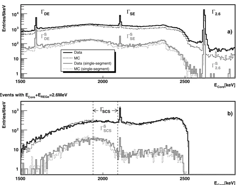
Fig. 2.E_Coredistributionsafor all coincident eventsbfor events withE_Core+E_REGe= (2614±5) keV. The 8 selected samples are indicated. The predicted distributions from the Monte Carlo are shown as well

tors around 2614.5 keV covers about three times the com- bined energy resolution (3σ) of the detectors. The geomet- rical acceptance for SCS events extends to 2110 keV, but SEP events would contaminate the sample, as they have a core energy of

= 2103.5 keV in this setup. They are excluded by removing events with the core energy of the seg- mented detector above 2090 keV. The

Tl decay also pro- duces 583.2 keV photons with a branching ratio of 84.5%. To avoid coincidences orginating from these photons an energy window of

583.2

3.0 keV is excluded.

The single-segment events are selected from each data sample by additionally requiring

– single-segment requirement:

|ESeg14−ECore|<

5.0 keV or

5.0 keV . The single-segment event samples are noted as

,

,

and

, respectively.

The coincidence trigger is only relevant for the

sample. However, the other samples are selected out of

the collected coincident events to ensure the same experi- mental conditions. In principle the REGe detector could also be used to tag 511 keV photons for events in the

and

samples. However, the statistics available is not sufficient.

The distribution of the energy of the core,

, of all coincident events is shown in Fig. 2a. The

distri- bution of all single-segment coincident events is shown in the same plot. Also shown are the simulated spectra which will be discussed in the next section. Figure 2b shows the

distribution for all coincident events with

+

= (2614.5

5.0)keV. The arrows indicate the

range corresponding to the acceptance angles for the

sample.

The DEP, SEP and 2.6 MeV peaks are all prominant in Fig. 2a. Only the SEP peak is also prominant in Fig. 2b.

The 511 keV annihilation photon that escapes the seg-

mented detector is fully absorbed by the REGe in these

events. The DEP peak disappears because the two 511 keV

428 I. Abt et al.: Test of pulse shape analysis using single Compton scattering events

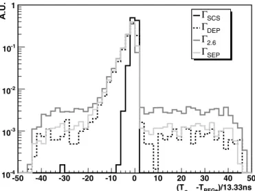
Fig. 3.T_Core−T_REGe distributions. The unit of thexaxis is the sampling clock

photons are emitted back to back and only one of the two photons can be tagged by the REGe detector. The numbers of events in all samples are given in the first row of Table 1.

The time between the arrival of the core trigger (T

) and the REGe trigger (T

), ∆T =

, is shown in Fig. 3. The ∆T distribution of the

events has a mean value of

9.4 ns with a RMS of 12.4 ns. Only one event falls outside the peak (

∆T

more than 8

13.3 = 107 ns). This confirms that events in the

sam- ple are predominantly induced by 2614 keV photons from the

Tl decay and the fraction of accidental coincidences is negligible at the 10

level.

The ∆T distributions of the

,

and

sam- ples are also shown in Fig. 3. These ∆T distributions are composed of “signal” peaks at ∆T

0 and flat distribu- tions of accidental coincidences. The “signal” events in the

and

samples register the 2.6 MeV photon in the segmented detector through pair production with one annihilation photon reaching the REGe detector. The “sig- nal” events in the

sample have another photon from the same

Tl decay registered in the REGe. The numbers of accidental coincidence events can be calculated by fit- ting the ∆T distributions with 133 ns

∆T < 266 ns with a constant function. The fractions of “signal” events after subtracting the accidental coincidence events are indicated by

and given in Table 1. The fractions of accidental co-

Table 1. The numbers of events in all data samples are presented in the first row. For theΓ_SCS sample,fcin the second row corresponds to the fraction of events with|∆T|<107 ns. The error on fccomes from statistics only. For theΓ2.6,Γ_DEPandΓ_SEP, it corresponds to the fraction of events in the central peaks of the|∆T|distributions after subtracting the accidental coincidence contribution.

The ratios of event numbers for data and MC are given in the third row with statistical errors only sample Γ_SCS Γ2.6 Γ_DEP Γ_SEP Γ_SCS^S Γ_2.6^S Γ_DEP^S Γ_SEP^S

#events 6716 25 780 6898 10 093 642 1131 1059 411

fc[%] >99 78_±1 87_±1 85_±1 97_±4 78_±2 87_±3 82_±4

# MC/data [%] 103_±1 66_±1 80_±1 79_±1 88_±3 70_±2 78_±2 73_±4

incidence events (1

) agree with the rough estimate of

≈

20% from the trigger rates, as explained in Sect. 2.1. No- tice, that most accidental coincidence events in the

,

and

samples can be treated as events triggered with only the core of the segmented detector and they are actually classified correctly. This was concluded in [1]

where a detailed study of core only triggered events was presented.

The

,

and

samples have wider ∆T dis- tributions than the

sample. This is an artefact of the fixed 100 keV energy threshold applied to the REGe detector. As the overall rise-time of a pulse, see Fig. 5a, does not depend on the energy, the time at which a fixed threshold is reached does. The

,

and

sam- ples are selected without any cut on

. This results in much wider spreads in

and thus in wider ∆T distributions.

2.3 MC simulation

The GEANT4 based Monte Carlo package MaGe [12] is used to simulate the setup. In order to speed up the com- putation only the

Tl decay is simulated and not the complete decay chain of the

Th source. The energies as deposited in the germanium detectors are smeared event by event according to the detector resolutions. The same energy thresholds and the coincidence trigger as for the measured data are applied to the simulated events. The MC is normalized to the data by counting the number of events within the energy region of

+

= 2614

5 keV, since events satisfying this requirement are almost exclusively induced by the 2614 keV photon from the

Tl decay (see previous section).

The simulated distributions of

are shown in Fig. 2a and b. The same selection cuts as required for the 8 data samples are applied to the MC events. The data to MC ra- tios are given in Table 1. They agree with the fractions of events with true coincident triggers (f

) within

10%. The overall excess of data of

20% for all but the SCS samples agrees well with the accidental coincidence rate.

2.4 Distinction between MSE and SSE in MC

The variable

is defined as the radius of the volume

that contains 90% of the total energy deposition in a ger-

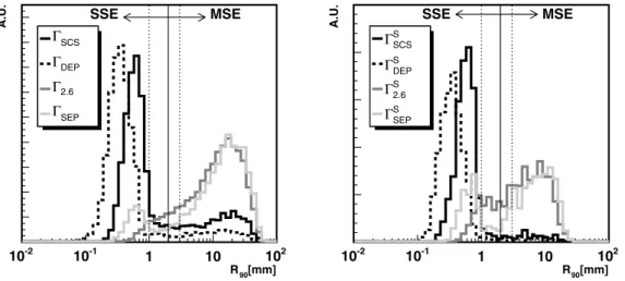
Fig. 4. R90 distributions of the 4 selected samples with- out the single-segment re- quirement (left) and with the single-segment requirement (right). The 3 vertical lines on each plot indicate theR90

values of 1, 2 and 3 mm

manium detector. It is used to study the size of the vol- ume within which the energy is distributed. Details are de- scribed in [8]. The distributions of

as calculated using MC information are shown in Fig. 4 for the 8 selected sam- ples. Events from

and

samples mostly have much smaller

than those from

and

samples.

ΓSCS

events have slightly larger

than

events due to the higher energy of the recoiling electron.

A fraction of the SCS events have relatively large

(> 2 mm). In most of these events the 2.6 MeV photon Compton scatters several times inside the segmented de- tector before reaching the REGe detector. They still sur- vive the

cuts due to the relatively large geometri- cal acceptance of the REGe detector. Events with

2 mm in the

sample originate from photons not in- teracting with the detector through pair production, but through multiple Compton scattering, and still depositing the same amount of energy as in DEP events. These events are significantly reduced by applying a single-segment cut, as shown in Fig. 4. The fraction of events from the

and

samples with

2 mm have the high energy photon depositing energy very locally. These fractions of events increase after applying a single-segment cut.

The “position resolution” of the DAQ is

1 mm, as ex- plained in Sect. 2.1. However, a conservative cut of

2 mm is used to distinguish SSEs from MSEs [1]. The frac- tions of SSEs (f

) in each sample are listed in Table 2.

The errors on

are estimated by varying the

cut value between 1 and 3 mm.

has a smaller fraction of SSEs than

, due to the relatively large selection win- dow. The

fractions for the

samples are larger than for the

samples, since the single-segment cut already re- moves most MSE events.

If only the segmented detector is used for triggering,

78% for the

sample, and

12% for the

sample [1] (89% and 30% for

and

samples, re- spectively). These values are similar to the ones for co- incident events. Therefore, even though accidental coinci- dences are not simulated by the MC, the

values as pre- sented in Table 2 can be used to evaluate the data samples collected with the coincidence trigger.

If the estimated 1 mm position resolution can be achieved through PSA, the SSEs from each sample should

Table 2. Fractionsf_SSE of events withR90<2 mm in each sample

sample ΓSCS Γ2.6 ΓDEP ΓSEP

fSSE 72⁺³₋₆% 10⁺⁶₋₇% 88⁺¹₋₂% 15⁺³₋₃% sample Γ_SCS^S Γ_2.6^S Γ_DEP^S Γ_SEP^S f_SSE 92⁺¹₋₃% 26⁺¹²₋₁₅% 96⁺¹₋₁% 31⁺⁶₋₅%

be correctly identified. The PSA procedure is described in the following section.

3 Pulse shape analysis

The same artificial neural network (ANN) package as used in [1] is used here to perform the pulse shape analysis.

The ANN is trained with an SSE sample against an MSE sample. In [1]

(without coincidence trigger) was used as the SSE-dominant sample and events in the 1620 keV line (with the 1620 keV photon from

Bi decay fully ab- sorbed in the segmented detector) as the MSE-dominant sample. The trained ANN was able to identify both SSE and MSE events with

85% efficiencies.

In this study, a similar analysis is performed. The ANN is trained with the

sample (SSE-dominant) against the

sample (MSE-dominant). The trained ANN is used to verify that the collected events in the

sample are SSE-dominant. The results are shown in Sect. 3.2 after a general description in Sect. 3.1.

In a second analysis the ANN is trained with the

against the

sample. It is shown in Sect. 3.3 that the results are consistent.

3.1 General features of the ANN

The core pulse of the segmented detector of a typical

event is shown in Fig. 5a. The rising part of the pulse con-

tains information about the event structure as explained

430 I. Abt et al.: Test of pulse shape analysis using single Compton scattering events

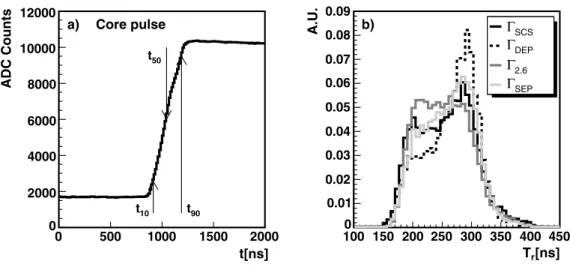
Fig. 5. a Core pulse of one DEP event, t10, t50 and t90

are indicated by arrows.

b distributions of the rise time Tr=t90−t10 for the 4 samples under consideration

in Sect. 1. The time

is defined as the time at which

the pulse has reached 50% of its maximum.

The 20 values before and the 20 after

are used for PSA. Thus, the selection of the 40 values is independent of the abso- lute amplitude of the pulse and thus independent of the energy.

t10

and

are defined as the times when the pulse reaches 10% and 90% of its maximum, respectively. The distributions of the pulse rise time,

=

, are shown in Fig. 5b.

is fully covered by the 40 values which cover a time window of 533 ns. The dominance of long rise- times in the

sample reflects the dominance of events close to the detector surface.

The ANN package as used here has 40 input neurons for the 40 pulse values. It has two hidden layers with 8 and 2 neurons each and 1 output neuron. The ANN is trained such that a large ANN output (N N

) indicates that the event is SSE-like and a small

indicates that it is MSE-like.

Since both

and

are related to the size of the energy deposition in the detector, a correlation be- tween

and

is predicted. On average events with small

should have large

and vice versa. It is clear that

is not the only variable that determines the pulse shape. Other, second order effects like the drift anisotropies caused by the crystal structure and inhomoge- nious doping concentrations also modify the pulse shapes.

Therefore, a 100% correlation between

and

is not expected. The details of this correlation can only be studied with a detailed pulse shape simulation which is be- yond the scope of this paper.

3.2 Verification of ANN training with single Compton scattering events

The ANN is trained with the

sample as SSE- dominant (signal-like) and the

sample as MSE- dominant (background-like). The training takes 300 itera-

3 Pedestals are subtracted by using the information during the 1µs interval before the trigger.

tions.

The trained ANN is then applied to all

and

events. It should correctly identify them as single–site and the multi–site events. The

distributions for all 4 samples are shown in Fig. 6a. The

distributions from the ANN trained with the

and

samples are shown in Fig. 6b.

The

events have in average larger

values than the

events. The peaks of the distributions are well separated. However, while the distribution for

events is quite similar to the one for

events, the distri- bution for the

events looks different from the one for

events. A shift of the peak is expected from the MC simulation, since there is a higher percentage of

events with

values above 2 mm indicating an MSE-like structure of the events, see Fig. 4. The

dis- tribution in Fig. 6 a in addition features a plateau towards high

values. This is probably an artefact of the spatial distribution of the events which are predominantly close to the surface which also influenced the ANN train- ing. This feature does not show up in Fig. 6b, most proba- bly due to the much lower statistics in the

sample.

The classification of events using the distributions de- picted in Fig. 6a (and b) is based on a cut in

,

. An event is classified as SSE-like, if

N N_out^CUT

, or MSE-like, if

. For a given value of

, the survival efficiency for any data sam- ple,

, is defined as the fraction of events in that sample that are identified by the ANN as SSE-like events.

The probabilities to correctly identify SSE- and MSE- like events,

and

, are calculated using the Monte Carlo predictions for the purities

of the sam- ples used, see Table 2, and using the measured

for the data samples. A linear dependence

=

+

is assumed. For a given

, the values for

are calculated for all samples, a linear fit is performed to ob- tain the slope and the line is extrapolated to

=1 to obtain

. It is extrapolated to

= 0 to determine 1

(see Fig. 6d for two fits). The fit procedure takes errors into account. The errors on

are listed in Table 2 and those on

are statistical only. The resulting

4 The ANN trained with 500 iterations gives similar results.

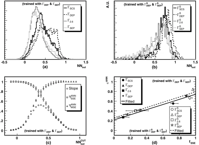
Fig. 6.Results of the ANN analysis, if the ANN is trained with theΓDEP(Γ_DEP^S ) sample as SSE-dominant and theΓSEP(Γ_SEP^S ) sample as MSE-dominant:aN Noutdistributions for all four samples. (ANN trained with theΓDEPandΓSEPsamples.)bN Nout

distributions for all four samples. (ANN trained with theΓ_DEP^S andΓ_SEP^S samples.)cη^ANN_SSE andη_MSE^ANNvs.N N_out^CUT. The fitted slopea, see text, is shown as well. Errors are taken from the MINUIT fit. (ANN trained with theΓDEPandΓSEPsamples. Results with theΓ_DEP^S andΓ_SEP^S samples are not shown here.)d^ANNvs.f_SSE;^ANNvalues correspond to the value ofN N_out^CUTgiving the maximum fitted slopea. Also given are results for the single segment samples indicated by^S(open points). See text for details

and

as a function of

are shown in Fig. 6c.

The fitted slope

is shown in Fig. 6c as a function of

as well. A clear maximum for

is visible.

The correlations between the values of

and

are shown in Fig. 6d for the value of

which maxi- mizes the slope

and

samples, the maximum value of

= 0.524

0.015 is achieved at

=0.37. The slope

does not ap- proach the ideal value of 1, indicating that

and

are not fully correlated. This is expected as the predictions for

are entirely based on the simple variable

as discussed in Sect. 3.1. The results for the single segment samples are also shown. They were subjected to the identi- cal analysis using the equivalent samples for training. The results of the fits are indicated for both single segment and unrestricted event samples.

The results for

and

are given in the first two rows of Table 3 with errors deduced from the fits. The ANN can correctly identify both SSE and MSE events at the 75%

to 80% level. The results for the single segment data sets

Table 3. η^ANN_SSE and η^ANN_MSE with the ANN trained with var- ious SSE-dominant samples against various MSE-dominant samples

ANN Training Analysis

SSE-dominant MSE-dominant η_SSE^ANN η^ANN_MSE Γ_DEP Γ_SEP 74.1_±2.7% 78.3_±2.8% Γ_DEP^S Γ_SEP^S 79.1_±7.2% 74.3_±6.8% ΓSCS Γ2.6 69.0_±2.1% 81.5_±2.5% Γ_SCS^S Γ_2.6^S 70.2_±4.3% 84.2_±5.1%

432 I. Abt et al.: Test of pulse shape analysis using single Compton scattering events

are similar to ones for the unrestricted samples. These re- sults agree in general with the values of

85% as achieved in [1].

The compatibility of the points with the linear fits in Fig. 6d leads to the conclusion that the SSE-like events in the

sample are identified with about the same efficiency as in the other samples. This is the most import- ant result of this study indicating that tagged SCS events can indeed be used to further study pulse-shapes in more detail.

As a cross check, the ANN was also trained with the

sample as SSE-dominant and the

sample as MSE-dominant. The same procedure with the trained ANN was then applied. The results are

= 80.5

2.9%

and

= 77.9

2.8%. These results are very similar to the values shown in Table 3, indicating that the training procedure is reliable and achieves consistent results.

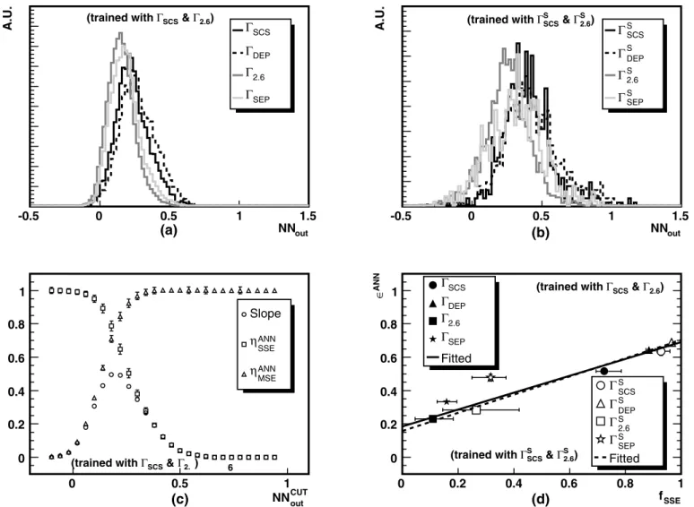
Fig. 7.Results of the ANN analysis, if the ANN is trained with theΓ_SCS(Γ_SCS^S ) sample as SSE-dominant and theΓ_2.6(Γ_2.6^S ) sample as MSE-dominant:aN Noutdistributions for all four samples. (ANN trained with theΓ_SCSandΓ_2.6samples.)bN Nout

distributions for all four samples. (ANN trained with theΓ_SCS^S andΓ_2.6^S samples.)cη_SSE^ANNandη_MSE^ANNvs.N N_out^CUT. The fitted slope a, see text, is shown as well. Errors are taken from the MINUIT fit. (ANN trained with theΓSCSandΓ2.6samples. Results with theΓ_SCS^S andΓ_2.6^S samples are not shown here.)d^ANN vs.fSSE;^ANN values correspond to the value ofN N_out^CUT giving the maximum fitted slopea. Also given are results for the single segment samples indicated by^S(open points)

3.3 Cross-check using SCS events for ANN training

The same procedure as described in the previous sec- tion is repeated with the ANN trained using the

(Γ

) as the SSE-dominant and the

(Γ

) as the MSE-dominant samples. The results are shown in Fig. 7.

The plateau feature in the

distribution from the

sample as seen in Fig. 6 a is much reduced, as shown in Fig. 7a. This is most probably due to the fact that events in the

sample have a relatively more uniform spatial distribution than the

events, resulting in a trained ANN which is insensitive to the spatial information.

The resulting identification probabilities

and

are given in the last two rows of Table 3. The ANN

can correctly identify SSE-like events at the 70% and MSE-

like events at the 80% level. This confirms again that the

selected SCS samples are enriched in SSE-like events and

can be used to train the ANN package.

4 Conclusions and outlook

Events with photons Compton scattering only once inside a germanium detector, SCS events, can be selected by tag- ging the scattered photon with a second germanium detec- tor. The pulse shapes of these events can be studied and used to test methods that distinguish between single-site and multi-site events.

In order to collect SCS events and perform pulse shape analysis, an 18-fold segmented prototype detector for the Phase-II of the GERDA experiment was positioned in front of a

Th source. A second germanium detector was posi- tioned to record the escaped photons at 72

, corresponding to 2040 keV energy deposit in the segmented detector, close to the Q-value of the 0νββ decay of

Ge.

According to the MC simulation

72% of the collected SCS events are true SSE events. The SSE-dominance is verified by an artifical neural network (ANN) trained in an independent way. These SCS events are then themselves used to train the pulse shape analysis package and thus the trained PSA is able to identify single- and multi-site events with efficiencies at the

80% level.

The studies can be improved in many aspects. The frac- tion of SSE events in the collected SCS sample can be increased by further improving the tagging method. For example, the whole experimental setup can be shielded from external photons and collimators can be positioned between the two detectors. In order to study the effect of the identification efficiencies on the sensitivity of double beta decay experiments (GERDA) the background events and their corresponding SSE and MSE fractions for the ex- periment under investigation need to be known in detail.

This requires a detailed MC simulation of the (GERDA)

experiment. A pulse shape simulation can improve the un- derstanding of the correlation between

and

. The use of individual pulses from neighbouring segments is expected to improve the identification efficiency. This was not considered in these studies. Detailed Monte Carlo simulations of the GERDA experiment and pulse shape simulations for the detectors are under way.

Acknowledgements. The authors would like to thank the GERDA and the Majorana Monte Carlo groups for their fruit- ful collaboration on the MaGe project.

References

1. I. Abt et al., Eur. Phys. J. C52, 19 (2007)

2. F. Petry et al., Nucl. Instrum. Methods A332, 107 (1993) 3. J. Hellmig, H.V. Klapdor-Kleingrothaus, Nucl. Instrum.

Methods A455, 638 (2000)

4. B. Majorovits, H.V. Klapdor-Kleingrothaus, Eur. Phys. J.

A6, 463 (1999)

5. D. Gonz˜alez et al., Nucl. Instrum. Methods A 515, 634 (2003)

6. S.R. Elliott, V.M. Gehman, K. Kazkaz, D.-M. Mei, A.R. Yong, Nucl. Instrum. Methods A558, 504 (2006) 7. GERDA Collaboration, S. Sch¨onert et al., Nucl. Phys.

Proc. Suppl.145, 242 (2005)

8. I. Abt et al., Nucl. Instrum. Methods A570, 479 (2007) 9. User’s Manual Digital Gamma Finder (DGF) PIXIE-4,

XIA LLC, http://www.xia.com

10. I. Abt et al., Nucl. Instrum. Methods A577, 574 (2007) 11. Canberra Reverse-Electrode Coaxial Ge Detector,

http://www.canberra.com/Products/494.asp 12. M. Bauer et al., J. Phys.: Conf. Ser.39, 362 (2006)