Worksheet 6: Computational Fluid Dynamics and Free Energy

Simulation Methods in Physics II SS 2019

Worksheet 6: Computational Fluid Dynamics and Free Energy

Kartik Jain

Institute for Computational Physics, University of Stuttgart

Contents

1 Introduction 2

2 Flow between two plates 2

2.1 Analytical solution . . . . 3 2.2 Computer simulations . . . . 3

3 Free Energy calculations 5

General Remarks

• Deadline for the report is Wednesday, 17th of July 2019, 12:00 noon

• In this worksheet, you can achieve a maximum of 20 points.

• The report should be written as though it would be read by a fellow student who attends the lecture, but doesn’t do the tutorials.

• To hand in your report, send it to your tutor via email.

– Kartik (kartik.jain@icp.uni-stuttgart.de)

• Please attach the report to the email. For the report itself, please use the PDF format (we will

accept MS Word doc/docx files!). Include graphs and images into the report.

• The report should be 5–10 pages long. We recommend using L

TEX. A good template for a report is available online.

• The worksheets are to be solved in groups of two or three people.

1 Introduction

This tutorial is divided in two separate parts: i)Fluid Dynamics ii)Thermodynamic integration. For the first two questions, you will study the laminar flow profile of a fluid between two infinite plates. For the last question, you may want to read parts of the book:

Understanding Molecular Simulation (2nd Edition), From Algorithms to Applications by Frenkel and Smit, 2001. Academic Press, ISBN: 9780122673511

From an ICP CIP-pool computer, you can find the seventh chapter under:

/group/sm/2018/tutorial_06/Frenkel-Smit-Chap7.pdf

2 Flow between two plates

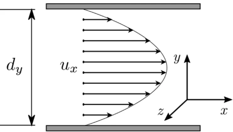
y

z x

Figure 1: The parallel plate geometry with the steady-state fluid velocity profile called the Poiseuille profile.

You need to characterize a microfluidic system that has microscopic length scales. The geometry under consideration consists of two fixed infinite parallel plates separated by a distance

shown in Fig. 1. The fluid has no-slip boundary conditions next to the walls (i.e. the fluid has zero velocity at the walls) given by

u(x, y

= 0, z) = 0

=

There is a constant force density

oriented in the positive

steady-state fluid velocity profile similar to that show in Fig. 1 is established. Thinking

ahead, this will be modelled in a periodic simulation box, thus there there is no pressure

difference across the system, i.e., the flow is only created via the external force density

.

2.1 Analytical solution

Task (6 points)

• Starting with the Navier Stokes equations shown in class (explicitly indi- cate all steps and assumptions.):

ρ

∂

∂tu

+ (u

=

+

+

∇ ·u

= 0,

derive the shape of the steady-state velocity profile.

• What is the maximum velocity? Where is it located?

• Write down the compressible and incompressible Navier-Stokes equations.

Discuss the macroscopic variable that differentiates these two forms of equations.

Hint

• You can assume there the fluid flow is in the

• You can assume there the fluid velocity profile only changes in

direction.

2.2 Computer simulations

The Navier-Stokes equations can be discretized by a number of methods like Finite Ele- ment or Finite Volume methods. The Lattice Boltzmann method (LBM) is a relatively new technique which discretizes the Boltzmann equation and recovers Navier Stokes equations under continuum limits of low Mach and Knudsen numbers. Here we will use the

You will need to compile

with either the GPU or CPU implementation. It is easiest to follow the installation steps from previous worksheets, but this time when editing myconfig.hpp, enable the three following features:

E X T E R N A L _ F O R C E S L B _ B O U N D A R I E S _ G P U

by removing the comment symbols ‘//’. If you are using a computer in the CIP pool, it is recommended to use the faster GPU implementation.

You will compare the numerical results with the analytical solution. The simulations

will take place in a periodic cubic simulation box of size 32

32

32. The walls are

modelled using an LB boundary which are placed at an offset of 1.5 between the top

and bottom limits resulting in

= 28 (between

= 1.5 and

= 29.5). You will need

to adapt the analytical solution by adjusting to these boundary conditions.

LBM Steady State

Now we can start with the real simulations. Take a look at and make sure to understand the template python script from the course webpage.

Task (5 points)

• Write the Lattice Boltzmann Equation

• Explain the concept of Particle Distribution Functions (PDF) and the relaxation parameter.

• Run the simulation for a force density:

= 0.01.

• Plot the fluid velocity at the center of the two plates together with the analytical maximum fluid velocity.

• Change the simulation time until it reaches a steady-state velocity (called convergence in fluid mechanical world). How many time steps were needed to achieve this steady state?

• Uncomment the second-last line in the script

lbf.print_vtk_velocity("{}/velocity.vtk".format(outdir)) and then rerun the simulation. This line writes a VTK output file on your current directory.

• Visualize this VTK file in the Paraview software. Figure out a way to cut two slices in the middle of the domain and then saving a screenshot.

What do you see? Please explain your observations in the report.

The velocity profile

Finally, the complete velocity profile can be measured. Make sure that the fluid has reached a steady state. The LBM is a transient algorithm and it requires a few time steps until the flow can traverse the whole geometry and the velocity profile (or pressure for that matter) reaches a steady state. Plot the velocity between the plates (on an arbitrary slice at

= 1, 2...31, 32).

Task (3 points)

• Measure the complete velocity profile for the force density

= 0.001.

• Plot the resulting velocity profile with the (adapted) analytical solution.

Do they match? Comment.

• Redo the steps above with force densities of

= 0.01 and

= 0.1. What

changes now? Do you need the same number of time steps to achieve a

steady state?

Hint

• Make sure to adjust the analytical solution with the boundary conditions from the simulations.

Fluctuations

Imagine you want to obtain the trajectory of a colloid undergoing Brownian motion in the slab-geometry you currently have setup. This can be done quite easily by adding this line: system.part.add(pos=(1,2,3), type=1) If you try it (go ahead, try it!), you will probably notice that the particle simply follows the velocity stream lines. The reason for this is that you have not set up a fluctating LB. For this task you do not need to add a particle, you just have to repeat the previous task with a fluctuating LB.

Task (4 points)

• Modify the value of kT in line

lbf = lb.LBFluidGPU(agrid=1, .... , kT=0.0) and replace it with a finite non-zero temperature kT=1.0.

• Reproduce the velocity profile you did in the previous task. You will need to average-out the fluctuations as much as you (reasonably) can. In other words, you will now not achieve a perfect steady state albeit the fluctuations will become more regular. Instead of reading from a single slice, try to take advantage of the velocity data in other LB nodes.

Hint

• It is okay to still have a bit of fluctuations in your final plot, use error bars to indicate the magnitude of the velocity fluctuations (i.e., the standard deviation).

• If you really want to see the Brownian trajectory of a colloidal particle (you don’t need to), you need to somehow keep them from crossing the LB boundaries.

3 Free Energy calculations

This question is taken from chapter seven from Frenkel and Smit, which covers compu- tational techniques to investigate the free energy. An alternative method for calculating the free energy difference between state

and state

is to use an expression involving the difference of the two Hamiltonians:

F_A−F_B

=

ln [hexp [−β (H

)]i

]

Task (2 points)

• Derive this equation.

Hint

• To derive the equation, start with Eq (7.1.1) of Frenkel and Smit.