Topological phenomena and proximity-induced superconductivity in carbon nanotubes

Topological phenomena and proximity-induced superconductivity in carbon nanotubes

DISSERTATION ZUR ERLANGUNG DES DOKTORGRADES

DER NATURWISSENSCHAFTEN (DR. RER. NAT.) DER FAKULTÄT FÜR PHYSIK DER UNIVERSITÄT REGENSBURG

vorgelegt von Lars Milz aus Düsseldorf

im Jahr 2018

Promotionsgesuch eingereicht am: 20.06.2018

Die Arbeit wurde angeleitet von: Prof. Dr. Milena Grifoni Prüfungsausschuss:

Vorsitzender: PD Dr. F. Bruckmann

1. Gutachter: Prof. Dr. M. Grifoni

2. Gutachter: Prof. Dr. C. Strunk

weiterer Prüfer: Prof. Dr. J. Fabian

Termin Promotionskolloquium: 07.12.2018

In liebevoller Erinnerung an Bella

„Can you hear me? It has been a glorious time to be alive doing research in theoretical physics. Our picture of the universe has changed a great deal in the last 50 years and I’m happy if I have made a small contribution. The fact that we humans who are ourselves mere

collections of fundamental particles of nature have been able to come as close to an understanding of the laws governing us and our universe is a great triumph. I want to share my excitement and enthusiasm about this quest. So remember to look up at the stars and not

down at your feet. Try to make sense of what you see and wonder about what makes the universe exist. Be curious. And however difficult life may seem, there is always something you can do and succeed at. It matters that you do not just give up. Thank you for listening.“

Stephen Hawking last words to the world (2018)

„This guy loves Majorana fermions! “

Simon Trebst about Alexei Kitaev (2017)

Teile dieser Dissertation wurden veröffentlicht:

Topology and zero energy edge states in carbon nanotubes with superconducting pairing, W. Izumida, L. Milz, M. Marganska, and M. Grifoni,

Phys. Rev. B, 96, 125414 (2017)

Majorana quasiparticles in semiconducting carbon nanotubes, M. Marganska, L. Milz, W. Izumida, C. Strunk, and M. Grifoni, Phys. Rev. B, 97, 075141 (2018)

Transverse profile and 3D spin canting of a Majorana state in carbon nanotubes, L. Milz, W. Izumida, M. Grifoni, M. Marganska,

Phys. Rev. B, 100, 155417 (2019)

Contents

Danksagungen iii

Abstract iv

Introduction 1

Outline 3

1. Topology in condensed matter physics 5

1.1. Geometric phase . . . . 5

1.1.1. Berry phase, connection and curvature . . . . 5

1.1.2. The Berry phase in Bloch bands . . . . 7

1.2. Symmetries and symmetry classes . . . . 7

1.2.1. Time-reversal symmetry . . . . 8

1.2.2. Particle-hole symmetry . . . . 9

1.2.3. Chiral symmetry . . . . 10

1.2.4. Symmetry classes . . . . 11

1.2.5. Classification of topological insulators and superconductors . . . . 13

1.3. Topological invariants . . . . 14

1.3.1. Winding number . . . . 15

1.3.2. Z

invariant . . . . 17

2. Majorana fermions and topological superconductivity 18 2.1. Introduction to superconductivity . . . . 18

2.2. Majorana fermions, Majorana zero modes and Majorana bound states . . . . 21

2.3. Topological superconductivity in p-wave superconductors . . . . 22

2.3.1. Kitaev chain . . . . 22

2.3.2. Topological invariants . . . . 25

2.3.3. Stability of Majorana bound states . . . . 25

2.4. Topogical superconductivity in semiconductor-superconductor hybrid systems 26 2.4.1. Semiconductor model . . . . 27

2.4.2. Superconducting bulk spectrum and topological phase diagram . . . . 30

2.4.3. Zero energy modes . . . . 32

2.5. Experimental realization . . . . 36

3. Carbon nanotubes 39 3.1. Structure of graphene and carbon nanotubes . . . . 39

3.2. Band structure of graphene . . . . 41

3.3. From graphene to carbon nanotubes - Curvature effects . . . . 43

3.4. Finite size carbon nanotubes . . . . 48

3.5. Four-band model: effects due to valley mixing and transverse magnetic fields 49 3.6. Two-band model . . . . 51

3.7. The lattice Hamiltonian in the helical-angular construction . . . . 54

3.8. Mean field approach of superconducting carbon nanotubes . . . . 57

4. Topological superconductivity in superconducting carbon nanotubes with time- reversal symmetry 60 4.1. Bulk spectrum of superconducting carbon nanotubes . . . . 60

4.2. BdG spectrum in finite-length zigzag class carbon nanotubes . . . . 65

4.3. Topological phase diagram . . . . 67

4.3.1. Winding number . . . . 67

4.3.2. Relation between Z and Z

invariants . . . . 72

4.4. Bulk-edge correspondence . . . . 73

4.5. Armchair class . . . . 76

4.6. Conclusion . . . . 76

5. Topological superconductivity in superconducting carbon nanotubes without time-reversal symmetry 79 5.1. Microscopic model . . . . 79

5.2. Bulk properties . . . . 81

5.2.1. Superconducting pairing in four-band model . . . . 81

5.2.2. Superconducting pairings in two-band model . . . . 84

5.2.3. Symmetries and topological invariants . . . . 87

5.3. Emergence of MBSs in finite nanotubes . . . . 90

5.4. MBS stability . . . . 92

5.4.1. Disorder . . . . 92

5.4.2. Magnetic field misalignment . . . . 93

5.5. Influence of the nearest-neighbor pairing ∆

. . . . 93

5.6. Majorana states at a phase boundary . . . . 95

5.7. Conclusion . . . . 98

6. Transverse profile and 3D spin canting of a Majorana state in carbon nanotubes 99 6.1. Symmetries of the Majorana spinor . . . . 99

6.2. 1D Majorana profile . . . . 100

6.2.1. Γ-point contribution . . . . 101

6.2.2. Fermi point contribution . . . . 102

6.2.3. 1D Majorana state . . . . 103

6.3. 3D Majorana quasiparticle wave function . . . . 104

6.3.1. Spin canting . . . . 109

6.4. Conclusion . . . . 112

7. Conlusion 113

A. Equivalence of topological invariants 115

B. Valley mixing 117

C. Analysis of the 1D continuum model 122

List of Figures 133

List of Tables 134

References 135

Danksagungen

Ich möchte mich bei Prof. Dr. Milena Grifoni für die Möglichkeit bedanken meine Doktorar- beit zu schreiben. Ich bin froh, die Chance gehabt zu haben an einem so interessanten Thema und in einer so tollen Gruppe zu arbeiten.

Ein weiterer großer Dank geht an Dr. Magdalena Marganska-Lyzniak für die Betreuung meiner Arbeit. Liebe Magda, ich habe die Zusammenarbeit mit dir die letzten fünf Jahre sehr genoßen. Mit dir die Übung für deiner Vorlesung Topology in condensed matter physics zu organisieren war sehr lehrreich und hat mir Spaß gemacht. Auch wenn wir uns Übungen ausgedacht haben, die wir selbst nicht lösen konnten.

Ebenfalls möchte ich mich bedanken bei Prof. Dr. Wataru Izumida. Er hat mein Verständnis vom Zusammenspiel von Topologie und Kohlenstoffnanoröhren auf ein neues Level gebracht.

Vielen Lieben Dank auch an meine Kollegen: Andreas Costa, Andrea Donarini, Tobias Frank, Maria Camarasa Gomez, Patrick Grössing, Petra Högl, Michael Kammermeier, Raphael Ko- zlovsky, Nico Leumer, Sebastian Pfaller, Sonja Predin, Benjamin Siegert, Sergey Smirnov, Matthias Stosiek, Davide Mantelli, Martin Wackerl, Heng Wang, Felix Weiner, Paul Wenk, Klaus Zollner und Allen die ich vergessen habe. Insbesondere möchte ich mich bei meinen Kollegen im Büro: Daniel Hernangomez Perez und Michael Niklas für die schöne Zeit be- danke. Weiter möchte ich mich bei Robert Hrdina, Sylvia Hrdina und Claudia Zange für die ganze Hilfe bedanken.

Auch ein Physiker hat mal Freizeit und daher danke ich meinen Freunden für die schöne Nicht-Physiker-Zeit mit euch. Bei Adrian und Basti für die ganzen Retro-Nerd Nächte mit sehr vielen Energiedrinks und LoL zocken.

Ein Dank geht auch an Dani, Domi, Jonas, Luzi und Phillip für die vielen schönen Abenden, die ich mit euch verbringen durfte. Weiter möchte ich mich bei Florian Geißler bedanken für die schöne Zeit auf Physikkonferenzen und außerhalb der Universität.

Ein lieben Dank geht an Chris und Steffi. Euer Sohn Ben ist wahrscheinlich das einzige Kind, dass ich kenne, welches Higgs-Feldtheorie total interessant findet. Ich hoffe noch auf viele weitere schöne Zeit mit euch.

Ein großer Dank geht an Bernhard, Kathi und Ulrike für eure ganze Unterstützung und das ihr mich sofort in eure Familie aufgenommen habt.

Besonders bedanke ich mich bei meiner kleinen Schwester Jana und meinen Eltern Johanna und Detlef Milz. Leider sage ich euch zu selten, wie toll ihr seid und wie froh ich bin euch zu haben. Daher denkt immer daran: Ohne euren Hilfe und Unterstützung wäre dies hier alles nicht möglich gewesen.

Zu guter letzt ein Dank an die Liebe meines Lebens: Felizia Merkau. Danke für alles! Ohne

dich hätte ich es niemals geschafft!

Abstract

Over the past decade Majorana fermions have been of great interest in condensed matter physics. Under special conditions they arise as quasiparticles in superconductors, where they are zero energy eigenstates of the Bogoliubov-de Gennes Hamiltonian and of the particle-hole symmetry operator. Theoretically such quasiparticles were predicted to appear in the elusive one-dimensional p-wave superconductors; but it is also possible to engineer s-wave systems in such a way that they mimic p-wave superconductivity. In this thesis we deal with the description and analysis of topological superconductivity in carbon nanotubes coupled to an s-wave superconductor.

In the first part we introduce the concept of topology in the condensed matter context.

Further, we discuss in a topologically nontrivial system the appearance of protected edge states, and we adress the so-called bulk-edge correspondence. Then, under the assumption of a short-ranged pairing potential, a mean-field Hamiltonian for the carbon nanotubes including curvature, spin-Âŋorbit coupling, valley mixing and a magnetic field is derived.

In the second part we analyse a minimal model for topological superconductivity in a carbon

nanotube with time-reversal symmetry. We can relate the number of edge states in the

superconducting finite length carbon nanotube to the corresponding topological invariant

and also prove the bulk-edge correspondence. Next we turn to a setup where time-reversal

symmetry is broken. In the presence of a perpendicular magnetic field and valley mixing the

topological superconducting phase diagram of semiconducting carbon nanotubes is shown. In

particular, regions in the magnetic field chemical potential plane possibly hosting localized

Majorana modes are discussed. Finally, we show that the spatial profile of Majorana bound

states can be derived analytically with good accuracy.

Introduction

The dynamics of many-body system can be understood by effective field theories describing the low-energy excitation of the system. Most systems are fermionic many-particle systems whose behavior is determined by a fermionic theory. Historically, fermionic effective field theories are well known due to the Landau-Fermi liquid theory and Landau theory of symmetry breaking.

Both theories are also called the „Standard model“ of condensed matter theory [1, 2].

In the Landau-Fermi liquid theory, the low-energy excitations are tranformed to the excited states of non-interacting fermionic system [3, 4]. Formally, such low-energy excitations - the so-called quasiparticles - are described as non-interacting fermions with renormalized proper- ties and the low-energy properties of the convectional metals, semiconductors, superconduc- tors and superfluids are determined by them. For example phonons, plasmons and magnons are well known quasiparticles in solids [5]. But also excitation like spinons and holons in Tomonaga-Luttinger liquids

are quasiparticles in condensed matter systems [6].

The Landau theory of symmetry breaking defines a classification scheme of phases of matter and the description of phase transitions [7, 8]. By definition, a phase of matter is a specific configuration of a many-body system and a transition between two phases is determined by discontinuities in the model. A discontuinity occurs because both phases have different symmetries, i.e. a phase transition is simply a transition that changes the symmetry.

However, due to the discovery of the integer [9] and fractional quantum Hall effect [10] new kind of phases occur in condensed matter physics. In general, the transition of quantum Hall states can not be classified by symmetry breaking theory, but by a quantity that describes the topological properties of the states [11]. The reason is that in contrast to Landau’s theory symmetry breaking, quantum Hall states have the same symmetries. The discovery of topological insulators was a breakthrough in this field, because topological insulators can be used for modern electronic circuits [12–14].

In 2016, D. J. Thouless and J. M. Kosterlitz won together with F. D. M. Haldane the No- bel Prize in physics for the description of topological effects in condensed matter theory. D.

J. Thouless, J. M. Kosterlitz and independently W. L. Berezinskii discovered the so-called Berezinskii-Kostelitz-Thouless (BTK) transition [15, 16]. In a two-dimensional superconduc- tors, the BTK transition is defined as a transition without spontaneous symmetry breaking in which vortices and anti-vortices are paired or not [2, 17]. Generally, topology consider the properties of topological spaces

, i.e. spaces that remain invariant under continuous defor- mations. There are several of categories of topological spaces. A good review about topology concepts used in physics can be found in Refs. [18–20].

In this thesis we are interested in gapped phases of quantum matter that can be distinguished

1 Tomonaga-Luttinger liquid is a system of interacting fermions in one-dimension.

2 These topological spaces do not necessarily have to be geometrical objects.

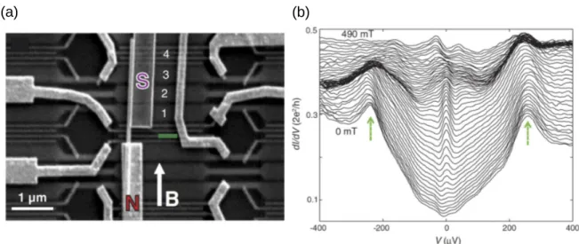
(a) (b)

Figure 1: (a) The experimental setup where an InSb nanowire is connected by normal and super- conducting contacts. (b) In the experiment the differential conductance

is measured as a function of the bias voltage V and the magnetic field. A zero-bias peaks appears for magnetic field at 100 mT.

One possible explanation of the zero-bias peak is the emergence of Majorana fermions. (Source: Ref.

[21]).

topologically. These kind of phases are called topological phases and can not be classified by the Landau’s symmetry breaking theory. Topological phases are characterized by a topological invariant in the bulk system. The transitions between them are called topological phase transitions. Thus, the BTK transition is a topological transition and the quantum Hall states are topological phases. From a topological point of view, two gapped states are equivalent if they can be adiabatically transformed without closing the energy gap and breaking the symmetries. Then it follows from the bulk-edge correspondence that gapless edge states emerge for a finite system [22].

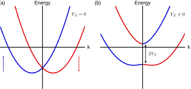
In topological superconductors, these gapless edge states behave similar to a Majorana fermion, known from elementary particle physics [23]. E. Majorana predicted an elementary fermionic particle which is its own antiparticle, and suspected that neutrinos could be one of these fermions. Nowadays it is known that neutrinos are not Majorana fermions. In condensed matter context, edge states in a topological superconductors are called Majorana fermions, because it is no longer possible to distinguish between quasiparticle and hole. The similarity results from the particle-hole symmetry in superconducors and the fact that the correspond- ing quasiparticles are superpositions of electrons and holes. In general, Majorana fermions can be described by a second quantized operator γ with the property γ

= γ. Their exis- tence has been predicted in various systems: p-wave superconductors [24], superfluid

He [1], topological insulator-superconductor hybrid systems [25], semiconducting nanowire - s-wave superconductor hybrid systems [26–29], quantum spin liquids [30] and also iron chains on s-wave superconductor [31].

In the following we will discuss mostly the nanowire proposals and their carbon nanotube

analogs. Although the experiments are by now very advanced [32], a definite proof that

the reported signatures [21, 33–36] are really due to the topologically nontrivial Majorana bound states (MBS) is still missing. The first experimental setup has been realized in the Delft group of L. P. Kouwenhoven, see Fig. 1(a), where an InSb wire is contacted with superconducting and normal metal electrodes. The existence of the Majorana bound state is probed by measuring the tunneling current I in dependence of the voltage bias V and an external magnetic field along the wire. A zero-bias peak emerging at a finite magnetic field is a hint of the possible existence of a Majorana bound state in the experiment see Fig. 1(b).

Majorana bound states have other unusual properties which are important for future electron- ics in quantum computing technology. In two-dimensional systems it can be shown that they are non-abelian anyons [37]. Anyons are quasiparticles whose many-body wavefunction ac- quires an arbitrary phase under exchange of two anyons [38]. While the nature of topological states of matter is interesting in its own right, the observation that systems with non-abelian anyons can be used to construct a quantum computer that is naturally immune to errors has focused much more attention in this field [39]. Basically, in a topological quantum computa- tion anyons are used for encoding and manipulating information non-locally which protects them from the influence of external perturbations [38].

Since the number of transistors in electronic circuits doubles every two years according to Moore’s law, further miniaturization will sooner or later encounter technical and physical limits. When reaching the scale of some nanometers, the size of molecules, quantum processes become important. Such sizes have already been reached by now. Additionally, the local heat production can impair the device operations and requires more effective cooling techniques.

Therefore, the industry researches a number of alternative device technologies where carbon based electronic elements play a major role [40]. A combination of carbon based electronic elements and quantum computing via non-abelian anyons might be a big revolution in future electronics.

Outline

This thesis is devoted to a description and analysis of topological superconductivity in prox- imitized carbon nanotubes. We discuss the topological origin of zero energy bound states in the two cases with and without time-reversal symmetry.

In the first chapter we will introduce topological concepts in the context of condensed matter physics. We discuss the question why we must use topological tools for certain state of matters and introduce the concept of geometric phases. Then, we show the correlations between the topological invariant, describing topological properties of the system, and the system’s symmetries. With this we are able to define topological invariants for specific systems.

The second chapter is dedicated to Majorana bound states in topological superconductors.

We prove the existence of these states in a one-dimensional p-wave superconductor, the Ki-

taev chain, and their emergence in nanowires with Rashba spin-orbit coupling and a parallel magnetic field in contact with an s-wave superconductor. At the end we discuss experimental realizations.

In the third chapter we describe how the electronic spectra of carbon nanotubes are obtained based on the dispersion relation of graphene, including curvature effects, spin-orbit coupling and the finite size of carbon nanotubes. Then, we investigate the effects of applied mag- netic fields and valley mixing in the energy spectrum of carbon nanotubes. Furthermore, we introduce a mean-field model of the superconducting correlations in carbon nanotubes.

In chapter 4 we investigate a minimal model for topological superconductivity in carbon nan- otubes. We discuss the emergence of edges states in the presence of time-reversal symmetry.

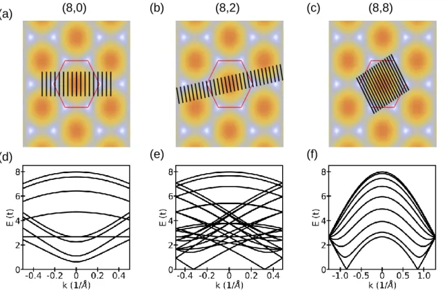
We notice that the formation of edge states depends not only on the chemical potential and the pairing potentials, but also on the chirality and the boundary shape of the nanotubes since they strongly affect the coupling of the two valleys. We show that the edge states emerge in the parameter region of nontrivial topological invariant. Finally, a 1D continuum model is introduced which allows us to obtain analytically the condition for the emergence of the edges states. By comparing it with the condition for nontrivial winding number, we find that these two conditions are identical, hence proving the bulk-edge correspondence.

We dedicate chapter 5 to the description of edge states in superconducting carbon nanotubes in the presence of a magnetic field. The starting point of our investigation is a microscopic tight- binding model for the carbon nanotube lattice, with external influences such as the substrate potential, superconducting pairings, magnetic field (perpendicular and axial) and disorder added in real space. The emergence of localized zero energy states above a critical magnetic field strength is demonstrated in the real space. Using the knowledge of the components of the wave functions, we prove the Majorana nature of the localized states. The effective model from chapter 3 allows us to gain the knowledge of the symmetries and topological invariants.

We construct the topological phase diagram and examine the stability of Majorana modes in the non-trivial phase.

The final chapter is devoted to the full 3D spatial profile of Majorana wave function in a

carbon nanotube - superconductor hybrid system. We show that it can be derived analytically

with great accuracy compared to the numerical results. We can also extract from it some

experimentally relevant information like the spin canting angle of a Majorana bound state,

which has been shown [41] to influence the electronic transport through a Majorana device.

1. Topology in condensed matter physics

In this chapter we introduce topological conecpts in condensed matter physics. We start with a review of Berry’s geometric phase and show the relations between symmetries of the systems and the possibility of topological properties in quantum systems. In the end we define the topological invariants which characterize topological properties. The results of this chapter have been published in Phys. Rev. B 96, 125414 (2017) and Phys. Rev. B 97, 075141 (2018).

1.1. Geometric phase

Sir M. Berry introduced a geometric phase, the so-called Berry phase, and explained the connection to classical electrodynamics [42]. He recognized that the phase factor is related to a gauge potential and depends highly on the path in the parameter space. The geometric phase is derived by the assumption of adiabtic transport and given by an abelian factor for non-degenerate eigenstates. However, the result of M. Berry can be generalized for degenerate eigenstates [43] and for non-adiabatic transport [44]. We discuss the formal derivation of the geometric phase done by Sir M. Berry for the case of a adiabatic abelian geometric phase.

Fore a more detailed account of geometric phases see Ref. [45].

1.1.1. Berry phase, connection and curvature

For the derivation of the Berry phase we consider a Hamiltonian H = H (R) which can be characterized by a vector of parameter R = (R

, R

, . . . ). This vector depends on the time t ∈ [0; T ] and moves adiabatically along a path C. Formally, the eigenstates |n (R)i can not be fully determined by the equation of motion H (R) |n (R)i = E

(R) |n (R)i since the U (1) gauge freedom of the eigenstate. We will assume that the phase of the eigenstate is well-defined and single-valued. Due to the adiabatic theorem [45], we must determine only the phase factor of the eigenstate which is described by the time-dependent Schrödinger equation

i ~ d

dt |Ψ

(t)i = H (R (t)) |Ψ

(t)i , where the solution |Ψ

(t)i is given by

|Ψ

(t)i = e

exp

− i

~ Z

0

dt

E

R t

|n (R (t))i . (1.1)

The energy-dependent phase is the well-known dynamical phase. The second phase is defined as γ

(t) = R

0

dR · A

(R), where the vector-valued function A

(R) is the corresponding

Berry connection. Formally, the Berry connection is given by

A

(R) = i hn (R (t))| ∂

∂R |n (R (t))i , (1.2)

and depends on the gauge. A gauge transformation yields

|n (R (t))i →

n

(R (t))

= e

|n (R (t))i ,

the Berry connection transforms to

A

(R) = A

(R) − ∂

∂R ζ

(R) .

Thus, the second phase γ

(t) will also transform γ

(T ) → γ

(T ) + ζ

(R (0)) − ζ

(R (T)).

In the case of a closed path, i.e. R (T ) = R (0), it follows ζ

(R (0)) − ζ

(R (T )) = 2πN with N ∈ Z , because e

is a single-valuedness function. Consequently, the phase angle γ

= γ

(T ) = H

C

dR · A

(R), known as the Berry phase, is a gauge-invariant quantity and can be measured in experiments [45].

In analogy to electrodynamics, the Berry connection can be interpreted as a magnetic flux.

Therefore, it is possible to define a gauge-invariant field strength tensor F

which is defined as

F

(R) = ∇

A

(R) − ∇

A

(R) , (1.3)

where ∇

=

µ

. The field stength tensor F

is known as the Berry curvature tensor. For a three-dimensional parameter space the Berry curvature and Berry connection are related by F

= ∇ × A

(R) with F

(R) =

F

(R), where

is the antisymmetric Levi-Civita tensor. Then, due to Stokes theorem the Berry phase can be expressed in terms of the Berry curvature. Explicity, the relation is given by

γ

= Z

S(C)

dS · F

(R) , (1.4)

with S (C) being a surface bounded by the closed path C. In contrast to the Berry phase,

which is defined on a closed path, the Berry curvature depends on the local geoemetry of the

parameter space given by the vector R. For degenerate eigenstates, the Berry connection is

defined as a matrix of dimension equal to the degeneracy.

1.1.2. The Berry phase in Bloch bands

Now we want to discuss a particular case of Berry phase physics related to solids. In several ex- periments the influence of the berry phase was measured. For example, in magneto-oscillatory effects [46, 47] or in one-dimensional systems, where the geometric phase is called Zak phase [48], in which the influence can be measured in adiabatic transport [49, 50] and the electric polarization [51, 52]. As discussed in the introduction, the physical behavior in solids can be understood by a non-interacting Hamiltonian H =

+V (r). Due to the periodic lattice po- tential V (r) = V (r + a), the electronic states fulfill the condition Ψ

(r + a) = e

Ψ

(r), where a is the Bravais lattice vector of the corresponding lattice, n the band index and

~ q is the crystal momentum belonging to the first Brillouin zone. Bloch’s theorem implies that the wave function can be written as u

(r) = e

Ψ

(r) wich satisfies the peri- odic boundary condition u

(r) = u

(r + a). In this new basis, the Hamiltonian becomes H → H (q) = e

He

where

H (q) = (p + ~ q)

2m + V (r) . (1.5)

Then the connection to the Berry phase is quite simple, since the parameter space is the first Brillouin zone, H (R) → H (q) with R → q and |n (R)i → |u

(q)i. Analogously, we can define also the Berry connection A

(q) = i hu

(q)| ∇

|u

(q)i and Berry curvature F

(q) = ∇

× A

(q). Both will be used later for the definition of the topological invariants.

1.2. Symmetries and symmetry classes

Until the 1980’s, only convectional phases are known which are described by Landau’s sym- metry breaking theory. Due to the discovery of the quantum Hall effect and later topological insulators, a new kind of phase, the topological phase, is introduced in the condensed matter context. In general, a topological phase of matter is defined as a state of a quantum system in which the bulk is described by a topological invariant and edge states emerges at the edges for a finite system. In order to understand the physics of topological phases we need to address the connection between symmetries and topological invariants.

There exist a zoo of topological phases which are characterized by different topological in- variants. The classification of topological phases can not be described by Landau’s symmetry breaking theory because topological different phases of a system has the same symmetries.

The topological properties of a system is classified by symmetry classes which depends on

the dimensionality and symmetries of the system. Here in this thesis we will introduce the

simplest classification scheme for gapped systems, like insulators and superconductors, with

a mean-field theory. Formally, a system is described by the following Hamiltonian

H = X

i,j

Ψ

H

Ψ

, (1.6)

where H

is the matrix element of the N ×N Hamiltonian matrix, Ψ

is the creation operator, Ψ

the annihilation operator and i the quantum number of the particle. Usually, the quantum number i includes the lattice position of the particle and the corresponding spin quantum numbers. For fermionic operators these operators obey the anticommutation relations

{Ψ

,Ψ

} = δ

and {Ψ

,Ψ

} = 0. (1.7)

In general, the system has certain symmetries, for example lattice symmetries, which can be grouped together in the group G. Then, for an element of the symmetry group g ∈ G exists a linear representation U = D (g), the symmetry operator, with U HU

= H or [U , H] = 0. Due to the Wigner theorem [53], symmetries can be only realized either by a unitary or antiunitary symmetry operator. In the case of an unitary symmetry operators, the Hamiltonian can be transformed into a block-diagonal form, where the blocks are labled as H

and λ is a certain irreducible representation of the corresponding symmetry group G [54, 55]. One well-known example is the lattic Hamiltonian for a solid. Due to the discrete translation symmetry of the lattice, the Hamiltonian can be brought into a block-diagonal form, where a block is labeled by the crystal momentum k.

For the classification scheme, we consider the block Hamiltonians H

and the corresponding behavior under anti-unitary symmetries. Then, the Hamiltonians can be classified depending on the absence or presence of antiunitary symmetries, which we will introduce next, and the dimensionality of the system. Then, the Hamiltonian is an element of the corresponding symmetry class. The term symmetry class was introduced in the random matrix theory and we will describe the connection to the topological properties and the symmetry classes later in this thesis.

The classification scheme describes the topological properties of an generalized system. Even in solids with a particular lattice structures, topological phases have a much more complicated nature [56–60]. Such systems are so-called topological crystalline insulators and superconduc- tors and can be also classified [61–63]. Furthermore We will show later in this thesis that the superconducting carbon nanotubes are an example of such a topological crystalline supercon- ductor.

1.2.1. Time-reversal symmetry

The first important symmetry for the topological classification of quantum matter is time-

reversal symmetry. By definition, the time-reversal transformation reverse the time T : t → −t

and commutes with the Hammiltonian [H, T ] = 0. Moreover, the time-reversal symmetry is an antiunitary symmetry which implies T = U

K with the property U

= U

, U

is a unitary matrix and K the complex conjugation operator. In general, every Hamiltonian is invariant when the time-reversal symmetry is applied twice. This implies T

= U

KU

K = U

U

= e

1 and U

= e

U

= e

e

U

= e

U

⇒ e

= ±1 by using U

= e

U

⇒ U

= e

U

. Thus, the time-reversal symmetry squares to T

= ±1 where for particles with integer spin it holds T

= 1 and T

= −1 for half-integer spin.

For a Hamiltonian with well-defined momentum k, time-reversal invariance is given by

T H (k) T

= U

H

(k) U

= H (−k) . (1.8)

The eigenstate Ψ (k) of the Hamiltonian H (k) is given by H (k) Ψ (k) = E (k) Ψ (k) with the energy E (k). In the case of time-reversal invariance, T Ψ (k) is an eigenstate of H (−k) with the energy E (−k). Due to Kramers theorem, which is important for topological insulators, every eigenstate for half-integer spin systems is doubly degenerate [64].

1.2.2. Particle-hole symmetry

In the case of superconducting system the mean-field dynamics is described within the Bo- goliubov - de Gennes (BdG) formalism, which we will discuss later in more detail. The BdG Hamiltonian, like all BdG Hamiltonians, is by construction invariant under a particle-hole operation. In general, the particle-hole operation maps the positive energy solutions onto their negative energy solutions. The BdG Hamiltonians with translational invariance which we will consider in this thesis are of the form

H

(k) = H

(k) ∆

−∆

−H

(−k)

!

, (1.9)

where H

(k) is the Bloch Hamiltonian and ∆ = −∆

is the pairing matrix. Like for the time-reversal symmetry also particle-hole symmetry is an antiunitary symmetry and can be represented by P = U

K with P

= ±1. Particle-hole symmetry leads to the condition

PH (k) P

= U

H

(k) U

= −H (−k) . (1.10)

which implies that the Hamiltonian anticommutes with P and the particle-hole symmetry

operator is given by P = τ

K, where τ

are the Pauli matrices. We can transform the BdG

Hamiltonian in the so-called Majorana basis, i.e. the basis of eigenstates of P , obtained by a

transformation U

, H

= U

HU

[22]. The unitary matrix U

is given by

U

= 1

√ 2

1 1

−i i

!

. (1.11)

The Majorana basis is important later for the definition of topological invariants. The particle- hole symmetry operator transforms as U

P U

= 1 K and the BdG Hamiltonian can be expressed as

iX (k) = 1 2

R

(k) + S

i (R

(k) − S

)

−i (R

(k) + S

) R

(k) − S

!

, (1.12)

where R

(k) = H

(k) ± H

(−k) = ±R

(−k) and S

= ∆ ± ∆

= −S

. Furthermore, it is possible to define a gauge transformation such that ∆ is a real matrix. Then it follows that S

= 2∆ and S

= 0.

1.2.3. Chiral symmetry

With both the particle-hole P and the time-reversal symmetries T , the Hamiltonian is also invariant under a product of both, i.e. C = T · P = U

U

. In contrast to previous discussed symmetries, the symmetry C, the so-called chiral symmetry or sometimes sublattice sym- metry, is given by an unitary symmetry operator and anticommutes with the corresponding Hamiltonian {H, C} = 0 with C

= 1. The absence of one of the symmetry leads to the absence of chiral symmetry. However, if both symmetry are absent then chiral symmetry can be either present or abesent.

In general, the chiral symmetry, connecting positive and negative energy solutions at the same momentum k which can be expressed in the following condition

CH (k) C

= −H (k) . (1.13)

For the eigenstate Ψ satisfying HΨ = EΨ there exists a paired state CΨ with the energy −E, that is, HCΨ = −ECΨ. In this thesis we will have BdG Hamiltonians of the form

H = H

(k) ∆

∆

−H

(k)

!

= H

(k) τ

+ ∆

τ

, (1.14)

where H

(k) is the Bloch Hamiltonian of the system with the property that there exist a

transformation U ˜ with U H ˜

(k) ˜ U

= H

(−k), ∆

= ˜ U ∆ ˜ U

is the real pairing matrix

and the chiral symmetry operator is given by C = τ

. In such a case we can use the chiral

symmetry to determine the spectrum of the system. The unitary transformation

U

= 1 2

1 + i 1 + i

−1 + i 1 − i

!

, (1.15)

rotates the Pauli matrices for the particle-hole basis as U

τ

U

= τ

, U

τ

U

= τ

and U

τ

U

= τ

. In this basis the chiral symmetry operator C ˜ = τ

is diagonal and the Hamiltonian is given by

H

(k) = 0 D (k) D

(k) 0

!

, (1.16)

where D (k) = H (k) −i∆

and we call this basis the chiral basis. Since H

(k) has a block-off diagonal form, H

(k) is block-diagonal. In order to obtain the energy spectrum we write down the BdG equation in chiral basis

H

(k) Ψ (k) = 0 D (k) D

(k) 0

! χ

(k) η

(k)

!

= ±E

(k) χ

(k) η

(k)

!

, (1.17)

where n ∈ {1, · · · , N } is the quantum number, like band index or spin index. The energies are positive E

(k) > 0 ∀n. Multiplying the equation from the left by H

(k) yields

H

(k) Ψ (k) = D (k) D

(k) 0 0 D

(k) D (k)

! χ

(k) η

(k)

!

= E

(k) χ

(k) η

(k)

!

, (1.18)

which follows from the block-diagonal form of the chiral symmetry. Thus, the eigenvalue problem can be reduced to solving the equation

det H

(k) − E

1

= det

D (k) D

(k) − E

1

= det

D

(k) D (k) − E

1

= 0.

Thus, the energy spectrum can be easily determined for systems with chiral symmetry. We will use this property later for the energy spectrum of superconducting carbon nanotubes.

1.2.4. Symmetry classes

Originally, E. Wigner introduced random matrix theory for the description of nuclear systems

[65, 66]. Later, random matrix theory was used to describe disordered systems in the context

of condensed matter physics. In general, random matrix theory can be used to determine

universal properties for different systems with the same symmetries. Formally, Hamiltonians

Classes Cartan label T

P

C

A (unitary) 0 0 0

Standard (Wigner-Dyson) classes AI (orthogonal) +1 0 0 AII (symplectic) -1 0 0 AIII (chiral unitary) 0 0 1 Chiral classes BDI (chiral orthogonal) +1 +1 1 CII (chiral symplectic) -1 -1 1

D 0 +1 0

BdG classes C 0 -1 0

DIII -1 +1 1

CI +1 -1 1

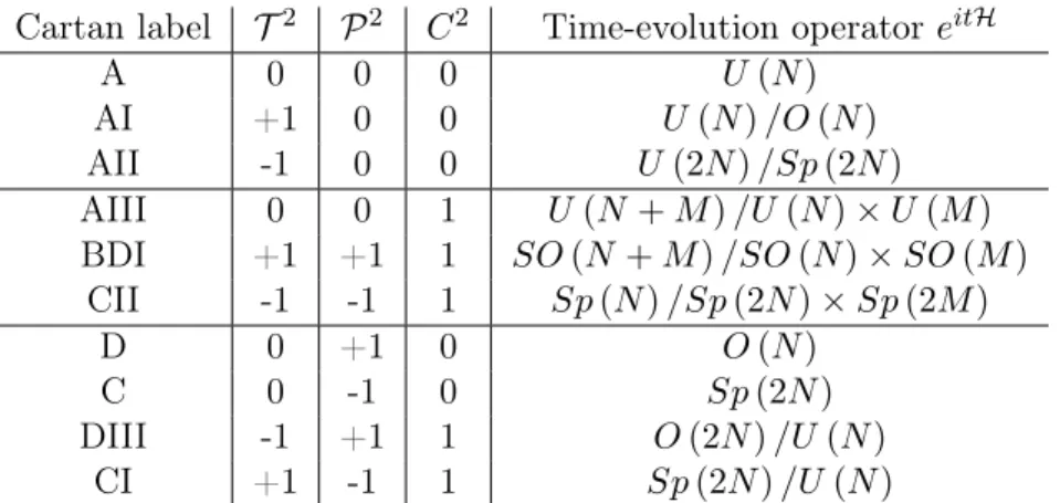
Table 1: The three chategories of the ten ranom matrix ensembles labled with the Cartan label. The ten ensembles can be characterized by the behavior of time-reversal T , particle-hole P and chiral C symmetries.

are assumed as random matrices. Therefore, random matrix theory is a good starting point of a classification of physical systems in mathematical physics.

At the beginning of random matrix theory, only one ensemble of random matrices was known.

Afterwards, F. Dyson generalized the idea of E. Wigner and introduced three ensembles by studying the behavior of random matrices under time reversal, where he demonstrated that the irreducible blocks are either unitary, orthogonal or symplectic matrices in dependence of the transformation which diagonalizes the matrix [67]. Due to chiral symmetry in quantum chromodynamics, three ensembles were added [68, 69] and later for systems with particle- hole symmetry, like superconductors, the final four ensembles were introduced [70]. Thus, the ensembles can be categoriezed in three groups as shown in Tab. 1. In total, there are ten different combinations of symmetries, see Tabel 1, and the behavior of the corresponding symmetry operators, discussed in the chapters of the corresponding symmetries. The labels of the ten ensembles are introduced by M. Zirnbauer [71]. He recognized the relation of the random matrix ensembles and so-called symmetric spaces by proving that the corresponding time-evolution operator e

with the Hamiltonian H is an element of the symmetric space.

The symmetric spaces are characterized by E. Cartan and labeled by the Cartan label [72, 73].

The result of E. Cartan is listed in Tab. 2 in the last column with the corresponding Cartan labels in the first column. In the context of the topological classification, the ten ensembles are also called symmetry classes and the result of the classification is called the tenfold way.

We will show the relation by two simple examples. Due to Stone’s theorem the time-evolution operator U

= e

∈ U (N ) a well-defined quantity ∀t ∈ R , where the N × N matrix is the Hamiltonian H of the system [74]. The group U (N ) is a Lie group and thus the Hamiltonian must be an element of the corresponding Lie algebra H ∈ u (N ). The first example is a system without symmetries. Then, the Hamiltonian is a Hermitian matrix which implies e

∈ U (N ). From Tab. 2 we see that this space is labled as A.

The second example is a system with time-reversal symmetry where T

= 1. For such systems,

the corresponding Hamiltonian can be brought into a real symmetric form. By definition, a

Cartan label T

P

C

Time-evolution operator e

A 0 0 0 U (N)

AI +1 0 0 U (N ) /O (N )

AII -1 0 0 U (2N ) /Sp (2N )

AIII 0 0 1 U (N + M ) /U (N ) × U (M) BDI +1 +1 1 SO (N + M ) /SO (N ) × SO (M )

CII -1 -1 1 Sp (N ) /Sp (2N ) × Sp (2M)

D 0 +1 0 O (N)

C 0 -1 0 Sp (2N )

DIII -1 +1 1 O (2N) /U (N )

CI +1 -1 1 Sp (2N ) /U (N )

Table 2: The relation of the ten random matrix ensembles and the corresponding spaces for the time-evolution operators.

general hemitian matrix H ˜ can be decomposed into a symmetric and antrisymmetric part H ˜ =

H ˜ + ˜ H

+

H − ˜ H ˜

= ˜ H

+ ˜ H

where H ˜

= ˜ H − H ˜

with H ˜

= − H ˜

. Since e

∈ U (N ) it follows that e

∈ O (N )

e

e

= e

e

= e

e

= 1.

Thzs, the time-evolution operator is given by e

∈ U (N ) /O (N ) which corresponds to the Cartan label AI.

1.2.5. Classification of topological insulators and superconductors

Non-interacting gapped systems were topologically classified using different methods. One method is to use the bulk-edge correspondence for the classification [22, 75], using the pres- ence of gapless edge states at the interface of two different phases. This method can be generalized for fermionic disordered systems using an effective low-energy field theory, the so-called nonlinear σ model. Originally, the term nonlinear σ model is introduced in the context of high-energy physics by M. Gell-Mann and M. Lévy. Later, F. Wegner derived non- linear σ models

for disordered systems [77], where the presence of topological gapless edge states implies further terms to the nonlinear σ model which evades Anderson localization [78]

and can be viewed as a physical proof of the bulk-edge correspondence [79]. The result for the topological classification in dependence of the spatial dimension and symmetry class is shown in Tab. 3. For differentiation between different topological ground states we can use topological invariants, which can be expressed in terms of the Berry connection or curvature.

3 There exists a remarkable correspondence between random matrix theory, a phenomenological theory for disordered systems, and the nonlinearσmodel [76].

Cartan label d = 1 d = 2 d = 3

A 0 Z 0

AI 0 0 0

AII 0 Z

Z

AIII Z 0 Z

BDI Z 0 0

CII Z 0 Z

D Z

Z 0

C 0 Z 0

DIII Z

Z

Z

CI 0 0 Z

Table 3: The result of the topological classification of the systems in dependence of the spatial dimensionality. Topological non-trivial systems can be characterized by an Z or a Z

topological invariant, respectively.

1.3. Topological invariants

For the definition of topological invariants, insulators and superconductors in the absence of disorder are considered, which implies a translational invariance. B. Simon noted that non-interacting gapped systems can be mathematically described as vector bundles and the Berry connection is the connection of a vector bundle and the Berry phase is equivalent to the corresponding holonomy [39, 45, 80]. Vector bundles can be classified by the so- called characteristic classes. With the characteristic classes it is possible to define topological invariants in terms of Berry connection and curvature for explicit calculations [18]. There are two important characteristic classes for the classification of physical systems. The first one is the so-called Chern class and the second one is the Chern-Simons class. In general, the Chern number is defined for systems with translational invariance in terms of the Berry curvature F of the system in the following way

Ch

= 1 n!

i 2π

Z

C

Tr (F

) ,

where n =

and C is the parameter space manifold. The Chern number is only defined for even-dimensional parameter space and without chiral symmetry. Therefore, the topological invariant coming from the Chern class is not the invariant which we need for describing the topological properties of the system studied in this thesis, a carbon nanotube. The fundamental topological invariant in 1D is Zak’s phase [48] in one band carrying a generic index n,

γ

= i 2π

Z

BZ

dk A

(k) , (1.19)

where A

(k) is the Berry connection in band n, A

(k) = hΨ

(k) |∂

|Ψ

(k)i, and |Ψ

(k)i is

the eigenfunction of a 1D bulk Hamiltonian for eigenvalue E

. We discussed that the Berry connection is gauge dependent quantity, so is Zak’s phase, and a gauge transformation changes γ

only by an integer. The more frequently used invariant is therefore W = exp (2πi P

l

γ

), where l are the indices of filled bands, which is gauge independent, although in general not quantized. The presence of discrete symmetries restricts the values which γ

can take. Mathe- matically, the Zak phase is the Chern-Simons invariant for the one-dimensional system which is defined as [18]

CS

= i 2π

Z

C

Tr (A) . (1.20)

The Chern-Simons invariant can be expressed in terms of the Berry connection A and in contrast to the Chern invariant well-defined for odd-dimensional parameter spaces C. In general, the Chern-Simons invariant is not quantized but due to the presence of symmetries it may take discrete values. In systems with chiral symmetry, in the gauge given by the chiral basis the winding number can be shown to be Z 3 w

= 2γ

, therefore W = exp(iπ P

l

w

) =

±1. In systems with particle-hole symmetry the topological invariant W can be evaluated using the representation of the Hamiltonian in the Majorana basis.

1.3.1. Winding number

Mathematically, the winding number is defined as quantity which counts how many times a closed curve circles around a point. The winding number is an important invariant for system with chiral symmetry. If the Hamiltonian has chiral symmetry {C, H} = 0, we have shown that one consequence is that in a basis where C is block-diagonal the Hamiltonian H has a block off-diagonal form (1.16). One can introduce the winding number as a one-dimensional topological invariant [81, 82]

ν = − 1 4πi

Z

BZ

dk Tr

CH ˜

(k) ∂

H

(k)

. (1.21)

Then, the winding number can be expressed only in terms of the Hamiltonian

ν = − 1 4πi

Z dk Tr

h CH ˜

∂

H

i

= 1 2π Im

Z

dk ∂

ln (det (D)) = 1 2π

Z

dk ∂

arg (det (D)) ,

where we have used the two relations Tr

D

∂

D

= ∂

ln (det (D)) and ln det D

=

Re (ln (det (D))) − iIm (ln (det (D))). Therefore, we see that the value of the winding number

depends on the trajectory of det (D) in the complex plane as k changes in the Brillouin zone.

Alternatively, it is also possible to define the winding number in terms of the flat-band Hamil- tonian [75]. For this we need the solution of the BdG equation in the chiral basis (1.18). The eigenfunctions Ψ

(k) of the Hamiltonian, with the eigenvalue ±E

(k), where − (+) refers to the filled (empty) state, can be written as [83]

Ψ

(k) = χ

(k) η

(k)

!

= 1

√ 2

u

±

n(k)

D

(k) u

!

. (1.22)

One can check that the function satisfies the BdG equation H

(k) Ψ

(k) = ±E

(k) Ψ

(k) with the relation D (k) D

(k) u

= E

(k) u

. A priori the eigenvectors u

may depend on k. Nevertheless, since u

are eigenvectors of D (k) D

(k) which is Hermitian, they form an orthogonal set. We can perform a unitary transformation into a basis in which DD

is diagonal, and the eigenvectors u

are independent of k. This transformation is continuous in k, which is assured by the continuity of the original eigenvectors u

(k). In the following, we shall work implicitly in that transformed basis. The projector onto the filled states is given by

P = X

n

Ψ

(k) Ψ

(k) = 1 2 1 − 1

2 Q. (1.23)

The operator Q acts as a flat-band Hamiltonian having the energy +1 for the empty states and −1 for the filled states independent of k since QΨ

(k) = (I − 2P )Ψ

(k) = ±Ψ

(k).

In the matrix form, we have

Q = 0 q (k) q

(k) 0

!

, (1.24)

where q (k) = P

l 1

En(k)

u

u

D (k) = U (k) D (k) and the matrix

U (k) = X

l

1

E

(k) u

u

(1.25)

has been introduced. Using the flat-band Hamiltonian, a winding number is defined as [75]

ν

= 1 2πi

Z

dkTr

q

(k) ∂

q (k)

, (1.26)

where the integral is taken over the whole one-dimensional Brillouin zone. The winding

number ν

counts winding of q (k). The proof of ν = ν

is presented in appendix A. The

connection to the Chern-Simons invariant (1.20) can be shown by using the fact that the

Berry connection of the system can be expressed as A = q

(k) ∂

q (k) with the chiral eigenstate (1.22) [84]. Therefore, due to chiral symmetry the Chern-Simons invariant is

of the winding number.

1.3.2. Z

invariant

We have shown that the winding number can be related to the Chern-Simons number by using the chiral symmetry. In one-dimensional systems with particle-hole symmetry the Z

topological invariant M = ±1 can be defined using the representation of the Hamiltonian in the Majorana basis (1.12). Hence, the topological invariant M is called Majorana number.

At the time reversal invariant momenta k ˜ = 0,

, X k ˜

, defined in Eq (1.12), it has the particularly simple form

X ˜ k

=





0 H

k ˜

− ∆

− h H

˜ k

+ ∆ i

0



 . (1.27)

where we used a gauge transform to transform the pairing matrix to a real matrix. We see that the matrix X

k ˜

is real and skew symmetric X ˜ k

= −X

k ˜

. For skew-symmetric matrices it is possible to define the so-called Pfaffian with Pf

h X

k ˜ i

= det

X ˜ k

. The topological invariant M can then be expressed through the Pfaffian of X (k) at ˜ k = 0,

. The relation due to the partucle-hole symmetry between the Chern-Simons invariant (1.20) and the Majorana number is derived in appendix A. Then, it follows

M = sgn Pf h

X π a

i

Pf [X (0)]

= (−1)

= ±1. (1.28)

With the Z

invariant we are able to determine the topological features of systems with

particle-hole symmetry. In the case of the superconducting carbon nanotubes we have particle-

hole symmetry and also chiral symmetry. Especially, we will show that in the presence of a

magnetic field, perpendicular to the nanotube axis, we can still use both invariants. The

winding number gives more information about the topological properties than the pfaffian

because it is a integer invariant and the pfaffian is a Z

invariant. Furthermore, the winding

number is more stable since a parallel magnetic field breaks the chiral symmetry. Thus, the

winding number is not well-defined anymore but the pfaffian is still defined. However, in the

case of a magnetic field parallel to the nanotube axis, the pfaffian turned out to be unreliable

because it only looks at k = 0 and k =

!

2. Majorana fermions and topological superconductivity

In this chapter we give a short overview of the BCS theory for superconductors. Then, we introduce Majorana fermions in quantum field and condensed matter theory. Majorana fermions, particles being their own antiparticle predicted already eighty years ago, have re- mained elusive to experimental observation so far. Hence, recent proposals to observe quasi- particles with the Majorana property in one-dimensional p-wave superconductor and s-wave superconductor hybrid systems containing semiconducting elements have raised big attention.

Further, we demostrate topological properties of both systems and the existence of Majorana states. Finally, we discuss realizations and signatures of Majorana states in epitaxially grown superconductor-semiconducting nanowires, which are by now the most advanced experimen- tally, and the emergence of a zero bias transport peak at finite magnetic field.

2.1. Introduction to superconductivity

Superconductivity is a quantum effect of many-body systems at low temperature which is defined by vanishing electrical resistivity and the presence of diamagnetism. Microscopically, superconductivity is driven by an attractive effective interaction between electrons near the Fermi surface. This leads to the formation of bound states with energy lower than the energy of two free electrons, which produces an instability of the Fermi sea. The attractive effec- tive interaction between electrons is a consequence of the electron-phonon coupling which dominates the electron-electron interaction due to screening effects.

The basic theory of superconductivity was formulated by Bardeen, Cooper and Schrieffer (BCS) in 1957 [85]. We introduce the BCS theory by considering the case of s-wave super- conductors. We start with the pairing Hamiltonian of an interacting electron system [86]

H − µN = X

k,s

ξ (k) c

c

+ X

k,k⁰

V

c

c

c

c

, (2.1)

where ξ (k) = ε (k) − µ is the single particle energy measured with respect to the chemical potential µ and

V

=







−V

< ~ω

for |ξ (k)| , |ξ (k

)| < ~ω

,

0 otherwise,

with ω

the Debye frequency. In general, the Coulomb interaction is repulsive and it is

screened in a metal. The screening of the Coulomb interaction can be described by the

random phase approximation [87]. The idea behind the BCS theory is that electrons interact

attractively V

> 0 within a small energy window in the vicinity of the Fermi energy. The

attractive interaction leads to a formation of bound states of two electrons in the electronic states |k ↑i and |−k ↓i which induces an instability of the Fermi sea.

Bogoliubov also realized that superconductivity can be understood with the help of mean-field theories [88]

. This approximation leads to the mean-field BCS grand canonical Hamiltonian

H

− µN = E

+ X

k,s

ξ (k) c

c

− X

k

∆ (k) c

c

+ ∆

(k) c

c

, (2.2)

where ∆ (k) = − P

k⁰

V

hc

c

i is the superconducting order parameter and E

the condensate energy. In the limit T → 0 E

is equal to the BCS ground state energy. In the mean-field Hamiltonian (2.2), the electron number is not conserved leading to eigenstates without definite electron number. In contrast, the pairing Hamiltonian (2.1) commutes with the electron number operator. In general, the number of electrons is conserved in supercon- ductors and it is possible to describe superconductivity with fixed electron number [89].

By introducing a new fermionic basis, the energy spectrum of the BCS Hamiltonian (2.2) can be analytically solved. The fermionic basis, the so-called Bogoliubov transformation, is defined in the following way

γ

γ

!

= u

(k) v (k)

−v

(k) u (k)

! c

c

!

, (2.3)

with |u (k)|

=

1 +

and |v (k)|

=

1 −

where E (k) = p

ξ

(k) + ∆

(k) is the quasiparticle energy. Due to the transformation above the BCS Hamiltonian (2.2) is diagonal and given by H

− µN = E

+ P

k,s

E (k) γ

γ

. It follows u (k) = u (−k) and v (k) = v (−k) for superconducting gaps with the property ∆ (k) = ∆ (−k). Quasiparticles in superconductors, sometimes called Bogoliubiv quasiparticles, are a superposition of particle and hole states for energies nearby the Fermi energy.

A generalized formalism is the Bogoliubov - de Gennes (BdG) formalism [86], where the effects of disorder or magnetic fields are included. By doubling the terms in the BCS Hamiltonian (2.2) we can define the Nambu spinor Ψ

=

c

,c

,c

,c

and the BCS Hamiltonian can be written as

4 Very often many-body systems cannot be described without approximations. One simple approximation is the mean-field approximation where a HamiltonianHAB=ABcan be approximated to the form

HAB→H_AB^MF=AhBi+hAiB− hAihBi,

which is known as the mean-field approximation. One of the most famous mean-field theory is the Hartree approximations [87] with A = c^†_k↑ck⁰↑ and B =c^†_k↓ck⁰↓. In the case of the BCS theory the mean-field approximation is given byA=c^†_k↑c^†_−k↓andB=c−k↓ck↑.

H

− µN = 1 2

X

k

Ψ

H

Ψ

+ const., (2.4)

where H

is the BdG Hamiltonian, which has the form

H

(k) =













ξ (k) 0 0 −∆ (k)

0 ξ (k) ∆ (−k) 0

0 ∆

(−k) −ξ (−k) 0

−∆

(k) 0 0 −ξ (−k)













. (2.5)

With the Nambu construction we map the Schrödinger equation for the system specified by the second quantized Hamiltonian (2.2) to an eigenvalue problem

H

(k) φ (k) = E (k) φ (k) , (2.6)

where φ (k) = (u

(k) , u

(k) , v

(−k) , v

(−k))

is the eigenvector and E (k) is the corre- sponding eigenvalue. This is the so-called Bogoliubov - de Gennes equation.

Finally, the BdG Hamiltonian satisfying the, in the previous chapter introduced, particle- hole symmetry PH

(k) P

= −H

(−k) where the symmetry operator is defined as P = τ

K with P

= +1. Therefore, if φ (k) is a solution of the BdG equation (2.6) with positive energy there exists a second solution φ

(k) = P φ (k) but with negative energy. We will call the solutions with positive energies quasiparticles and the solutions with negative energies holes. Thus, the particle-hole symmetry operator maps quasiparticles to holes.

In this thesis we consider systems that are not intrinsic superconductors. By coupling an s-wave superconductor to a normal conductor, the conductor becomes superconducting. This is the well-known proximity effect and can be described by Andreev reflections [90]. The microscopic model of the proximity effect is defined by the tunneling Hamiltonian

H

= X

s,σ

X

hi₀,j0i

t

c

0m

d

+ t

d

0,σ

c

, (2.7)

where c

is the normal conductor creation operator at the lattice site i with spin quantum

number s, d

the corresponding superonductor creation operator at the lattice site j with

spin σ. By integrating out the superconductor operators, an effective model is derived for the

normal conductor, including superconducting pairing and a renormalized chemical potential

[91–95].