Effects of Occupants and Local Air Temperatures as Sources of Stochastic Uncertainty in District Energy System Modeling

(1)

Journal Article

Effects of Occupants and Local Air Temperatures as Sources of Stochastic Uncertainty in District Energy System Modeling

Author(s):

Mosteiro-Romero, Martín; Schlueter, Arno Publication Date:

2021-04-19 Permanent Link:

https://doi.org/10.3929/ethz-b-000479415

Originally published in:

Energies 14(S 8), http://doi.org/10.3390/en14082295

Rights / License:

Creative Commons Attribution 4.0 International

This page was generated automatically upon download from the ETH Zurich Research Collection. For more information please consult the Terms of use.

ETH Library

(2)

Article

Effects of Occupants and Local Air Temperatures as Sources of Stochastic Uncertainty in District Energy System Modeling

Martín Mosteiro-Romero^∗,† and Arno Schlueter

Citation: Mosteiro-Romero, M.;

Schlueter, A. Effects of Occupants and Local Air Temperatures as Sources of Stochastic Uncertainty in District Energy System Modeling.Energies 2021,14, 2295. https://doi.org/

10.3390/en14082295

Academic Editors: Francesco Causone, Alfonso Capozzoli

Received: 10 March 2021 Accepted: 15 April 2021 Published: 19 April 2021

Publisher’s Note:MDPI stays neutral with regard to jurisdictional claims in published maps and institutional affil- iations.

Licensee MDPI, Basel, Switzerland.

This article is an open access article distributed under the terms and conditions of the Creative Commons Attribution (CC BY) license (https://

creativecommons.org/licenses/by/

4.0/).

Architecture and Building Systems, ETH Zurich, Stefano-Franscini-Platz 1, 8093 Zurich, Switzerland;

schlueter@arch.ethz.ch

* Correspondence: mosteiro@arch.ethz.ch

† Current address: Department of Architecture, School of Design and Environment, National University of Singapore, 4 Architecture Drive, Singapore 117566, Singapore.

Abstract: Input uncertainty is one of the major obstacles urban building energy models (UBEM) must tackle. The aim of this paper was to quantify the effects of two of the main sources of stochastic uncertainty, namely building occupants and urban microclimate, on electrical and thermal supply system sizing at the district scale. In order to analyze the effects of the former, three different methods of occupant modeling were implemented in a UBEM. The effects of the urban heat island on system sizing were studied through the use of measured temperature data from a weather station in the case study district compared to measured data from a national weather station. The methods developed were used to assess the sizing and costs of centralized and decentralized technologies for a case study in central Zurich, Switzerland. The choice of occupant modeling approach was found to affect the district’s total annualized costs for space heating and cooling by±5%, whereas for the costs of electricity the variation was±8%. Regarding outdoor temperature, the effects on the heating demands proved be negligible, however the costs of the cooling alternatives were found to vary by about 4% at the district scale due to the effect of urban climate, for individual buildings this deviation was as high as 40%.

Keywords: energy simulation; urban energy system modeling; building occupant modeling;

urban climate

1. Introduction

District energy systems can be one of the least-cost and most-efficient solutions for reducing primary energy demand and greenhouse gas emissions, with the potential to contribute up to 58% of the required CO2emission reductions required in the energy sector by 2050 [1]. Interconnecting buildings through district-scale energy systems provides opportunities to exploit synergies between buildings with different uses and demand profiles, as well as allowing the integration of distributed energy producers. Achieving these benefits, however, requires a detailed understanding of the types and dynamics of energy demand in buildings at high spatial and temporal resolution.

Urban building energy modeling (UBEM) can be a powerful tool to assess the current and projected demands of urban areas in order to support the planning of interventions at a variety of scales, such as building retrofits, urban form modifications and district energy system implementation. Building energy modeling is a well-studied field, with a number of software tools that have become an integral part of the planning process. Due to the large amounts of data required to create a bottom-up model of a single building, simply using building-scale tools to create individual building energy models for each building in an urban area would make data collection impractically onerous [2]. Furthermore, urban areas cannot be simply analyzed as an aggregation of single buildings as complex interactions between the components of the urban system arise when scaling from the

Energies2021,14, 2295. https://doi.org/10.3390/en14142295 https://www.mdpi.com/journal/energies

(3)

building to the urban scale, such that traditional building energy modeling methods cannot be implemented [3].

Currently, the two major obstacles UBEM must tackle are input data availability and input uncertainty [4]. In order to reduce the amount of data required to create a model, UBEM typically use archetypes to represent a number of buildings with similar properties [2]. However, such simplifications can increase the uncertainty in the simulated results as the actual properties of the specific buildings being modeled are not known.

Uncertainty in building energy demand models can be classified as epistemic or stochastic [5]. The former arises as a result of lack of knowledge about specific input parameters, such as the thermal properties of the building envelope, lighting and appliance power densities, or supply system efficiencies. With the increased availability of sensor data in cities, the contribution of epistemic uncertainty can be better quantified through measurement campaigns. Optimization-based methods [6], pattern-based methods [7], and Bayesian calibration methods [8] combined with meta-modeling [9] can then be used to reduce the error in building energy predictions. Such methods have been implemented at the urban scale, in particular in the calibration of archetypes through Bayesian calibration [10] or the use of surrogate modeling to estimate unknown building properties [11].

Stochastic uncertainty, on the other hand, arises as a result of the inherently random nature of parts of the system under analysis. Due to their aleatory nature, it is impossible to predict future variations in stochastic sources of uncertainty, and hence it can be better characterized but not reduced by measurement campaigns [5]. Thus, methods to analyze and quantify the role of these sources of uncertainty on the planning of energy systems at the urban scale need to be developed. The primary drivers of stochasticity in building energy simulation are building occupants and climate [12]. The roles of these sources of uncertainty are analyzed further in the following sections.

1.1. Occupants

Occupant behavior is one of the key drivers of the so-called performance gap in energy model predictions compared to measured consumption data. For example, previous research found that occupant behavior could lead to a 100% variation in the energy demands of identical buildings [13]. Thus, modeling occupants is crucial for predicting the energy demands in buildings as well as in order to analyze the effects of changes in an area’s activities on the corresponding energy infrastructure required.

Occupants in building energy modeling have traditionally been represented through deterministic schedules that indicate typical patterns of occupant presence and appliance use at each time of the day for different building use types. Such schedules can typically be obtained from standards (e.g., [14,15]) and provide a simple input for simulations. However, the use of the same profiles for all spaces of a given function can lead to homogeneous load profiles that misrepresent the true peak loads in a district. Since energy systems are typically sized in order to meet buildings’ or districts’ peak demands, such unrealistic homogeneous loads can lead to sub-optimal system sizing and consequently inefficiencies in system operation. In order to account for the inherent uncertainty in building users’

actions, a number of stochastic methods for occupant modeling have been proposed.

Agent-based modeling approaches further seek to predict occupants’ behavior, interactions, and adaptation to their environment. At the district scale, however, the majority of the works in the literature show a reliance on deterministic schedules of occupant presence and appliance use. There are only a few stochastic models in the literature, and each of those approaches covers only one building use type [16].

While increasingly complex methods to model occupant presence and behavior at the building scale have been developed, Tahmasebi and Mahdavi [17] showed that simulation results depended primarily on the availability of occupant presence data rather than whether deterministic or stochastic representations of occupancy patterns were used.

When scaling up to the district scale, however, the number of people to be monitored is multiplied, exacerbating the difficulty of data collection on individual occupants. The

(4)

widespread availability of data from location-based services might provide a useful source for the development of data-centric approaches [18], however such approaches remain, as of yet, restricted to the prediction of occupancy for a limited number of building use types.

New methods are required to model occupants in urban areas for a variety of building use types. These methods should consider the effects of occupants’ location-based activities as well as the interactive effects of building energy consumption and mobility [19]. Increas- ingly, transportation models that predict people’s movements in urban areas based on their individual characteristics and activities are used in urban planning. Such microsimulations could serve as a source for occupant and activity modeling in buildings to help improve energy demand predictions in districts [20].

1.2. Climate

Climate data are a fundamental input into any building energy simulation. In order to avoid the biases caused by yearly variations in weather data, these inputs usually take the form of a typical meteorological year (TMY) based on long-term observations of the local weather station. Such data are usually smoothed and averaged or even entirely based on statistics, thus ignoring the modifying effect of the surroundings [21]. This allows equipment sizing to be carried out in order to be able to meet energy demand under

“normal” operating conditions. However, the unpredictability of actual weather adds uncertainty to the simulation results, potentially leading to systems that cannot cope with actual demands after construction. TMY data are based on past observations that might no longer be representative of actual whether conditions throughout the lifespan of systems planned to last for decades. Increasing concern is being shown that a single data file cannot contain sufficient information on plausible weather conditions [5].

Furthermore, these processes can lead to increased temperatures in urban areas compared to rural ones, a phenomenon known as the Urban Heat Island (UHI) effect. Com- pounded by global warming, the UHI can lead to a significant increase in cooling demand in urban areas [22,23]. These variations in air temperature patterns, wind speed, and solar radiation in urban areas are generally overlooked in building energy demand models.

Previous studies on the effects of local environmental conditions on energy consumption have however largely focused on the individual building scale [23]. Indeed, most currently available UBEM do not account for building emissions heating up the local microclimate and the latter’s consequent effect on the building energy demand [19]. Meanwhile, when district-scale energy demand simulations are coupled to urban climate models, they usually rely on simplified assumptions [24]. These are typically at the mesoscale, which means they can predict climate phenomena in the 100 km order, i.e., at the city scale [25].

Planning district heating and cooling systems requires a detailed understanding of the cooling loads in a given district. In order to achieve this, each building and its surrounding environment need to be simulated at the micro scale. Existing microclimate simulation tools are, however, extremely computationally expensive, restricting the modeling of urban microclimate at the district scale to sub-yearly time frames [26].

1.3. Goal and Scope of This Paper

The uncertainty caused by occupants and climate will continue to have a considerable impact on the results obtained in district-scale energy demand simulation. Previous papers have explored the effects of occupant modeling approaches on the demands predicted by the UBEM City Energy Analyst (CEA) [20,27]. In addition, the effects of the urban heat island on the space cooling demand were analyzed by connecting CEA to microclimate simulation ENVI-met [28,29]. The computational expense of the microclimate simulations, however, restricted the analysis to a single day. While this approach provided insight into the demand dynamics under extreme weather conditions, general conclusions on the implications for energy systems could not be extracted from the limited scope provided by a single day’s worth of results.

(5)

The goal of this paper was to quantify the effects these variations in demand patterns cause in the sizing and costs of different energy supply systems. The analysis of these stochastic sources of uncertainty on the planning of energy supply systems is carried out both at the district and building scale in order to assess whether the effects could be large enough to affect planning decisions in each case.

Photovoltaic (PV) systems, heat pumps, chillers, and thermal networks were selected as the most promising technologies for the selected case study. The aim is to compare the effects of the various occupant and climate assumptions on the planning of a theoretical centralized district energy system compared to decentralized alternatives. In order to observe the effects of each of these sources of uncertainty on each energy system individually, system integration was not considered. For example, the effects on the cooling demands were only considered for the cooling system performance, whereas the consequent effects on the electricity demand for cooling were not considered. Therefore, while occupancy was assumed to affect both PV and thermal system performance, urban climate effects were only considered for thermal systems.

The CEA technology simulation tools used are described in Section2. These are subsequently applied to the case study area presented in Section3. Section4.1presents a summary of the effects of occupants and outdoor temperature on the case study area’s demands. The effects of occupants on the performance of solar photovoltaic (PV) systems and electricity costs are subsequently analyzed in Section4.2. District heating and cooling networks as well as decentralized system alternatives are analyzed in Section4.3, accounting for deviations caused by occupant modeling and local climate. The results are further discussed in Section5before presenting overarching conclusions in Section6.

2. Materials and Methods

District energy modeling and supply system simulation were carried out using the City Energy Analyst (CEA), an open-source software for the analysis and optimization of urban energy systems [30]. The tool uses a simplified, single thermal zone resistance- capacitance model for building energy demand forecasting. The software additionally includes a number of tools to estimate renewable energy resource potentials and system technology sizing and simulation. This paper focuses on the effects of occupants and the urban heat island effect on heating, cooling, and electricity demands and on the planning of their corresponding supply systems. In order to quantify the effects on system performance and costs, two of the CEA technology models were used, namely the solar potential and thermal network tools.

2.1. Occupant Modeling Approaches

The effects of occupancy modeling on the planned systems are explored by comparing the results for three different modeling approaches: deterministic, stochastic, and population-based (PopAp). The models and their effects on the energy demands of the current case study area have been discussed in a previous paper [20], so they are only briefly introduced here.

The deterministic approach consists of assigning the number of occupants and the demands for electricity and domestic hot water at each hour of the year according to fixed schedules taken from standards [31]. This means, however, that each building’s occupancy depends solely on its function, with no variation between one weekday and the next. In order to add temporal diversity to the occupancy patterns, we implemented Page et al.’s occupant presence model [32] in CEA. Occupant presence is modeled as a two- state Markov process, where each building occupant can either be “absent” or “present”.

The implementation in CEA uses the same standard schedules as an input to calculate transition probabilities between these two states for each building occupant at each hour of the year and consequently randomly assign occupant presence at each hour. By creating individual schedules for each person in the district, this approach accounts for the random variations in occupancy patterns. However, each building’s unique characteristics are not

(6)

captured, as buildings with the same use type will still tend to have the same occupancy patterns on the aggregate.

A third, population-based approach (PopAp) for occupant modeling was defined in order to overcome these limitations. This method adds diversity between different buildings of the same occupancy type by using data about the actual occupants in the case study area. Inspired by agent-based transportation models, a population of occupants is first created, and each of them is then assigned a daily plan comprising a set of activities along with their start and end times (tstartandt_end), and a location where each activity is taking place. For the case study under consideration, presented in Section3, the majority of building occupants were students and employees. The population of occupants required for the PopAp method was defined based on employee registers and course enrollment data. The available activities to be assigned to each of them were limited to “work”,

“study”, or “lunch”.

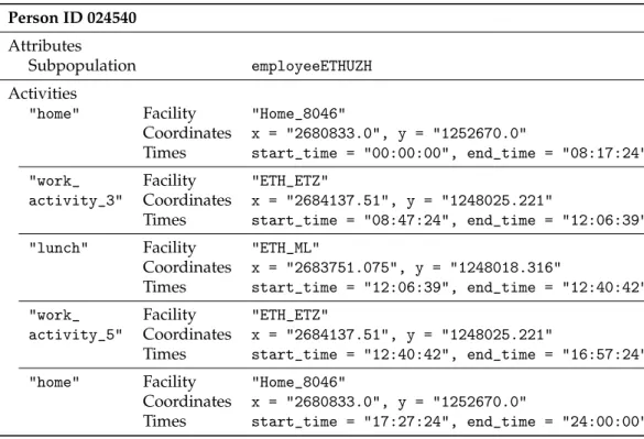
Table1shows a sample employee’s attributes and activities. Each employee was assigned a workspace, which assumed to be located in buildings that included either office, lab, or hospital functions. For each employee’s workday, the starting and ending time were assigned randomly from a normal distribution:tstart∼N(9:30, 1.7)andtend ∼ N(_{17:00, 1.7}). For the “study” activity type, both the start and end times as well as the location were assigned based on the course enrollment data. No weekend occupancy was assumed for students and employees.

Additionally, vacation weeks were assigned randomly to students and employees according to the national average yearly vacation time [33]. At the beginning of each week, whether an occupant started such a period of long absence was defined by comparing a randomly-drawn number to the monthly probability of occupant presence from the national standards [15]. The full set of assumptions in each occupancy model can be found in AppendixA. Out of the three approaches considered, the PopAp case is assumed to provide a more realistic depiction of occupant presence and activities in the case study area, as it is the only one that is based on locally-collected data rather than national standards.

Table 1.Sample data for a university employee in the case study area.

Person ID 024540 Attributes

Subpopulation employeeETHUZH

Activities

"home" Facility "Home_8046"

Coordinates x = "2680833.0", y = "1252670.0"

Times start_time = "00:00:00", end_time = "08:17:24"

"work_ Facility "ETH_ETZ"

activity_3" Coordinates x = "2684137.51", y = "1248025.221"

"lunch" Facility "ETH_ML"

Coordinates x = "2683751.075", y = "1248018.316"

"work_ Facility "ETH_ETZ"

activity_5" Coordinates x = "2684137.51", y = "1248025.221"

"home" Facility "Home_8046"

Coordinates x = "2680833.0", y = "1252670.0"

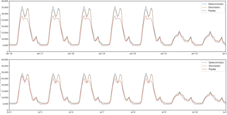
The number of building occupants in the district along a typical summer and winter week are shown in Figure1. Given that the CEA demand model is based on a single

(7)

thermal zone representation of each building, only occupant presence or absence was considered in all cases. The demands for appliances were associated to occupant presence by simply assigning an electrical demand to occupants of each type (employees and students). Occupant presence furthermore affects building system controls such as the ventilation rate, which depends on the number of occupants in a building, as well as the room temperature, since the buildings’ systems are set to their set point temperature whenever at least one occupant is present. Finally, the presence of occupants and their use of appliances leads to sensible and latent gains, which in turn affect the thermal loads of each building.

, , , , , , , ,

Figure 1.Number of occupants in a winter (top) and summer week (bottom) for each of the occupant modeling approaches.

2.2. Effects of Urban Climate

In a previous study, the effects of urban microclimate on the space cooling demand of the area were estimated by connecting CEA to microclimate simulation ENVI-met [28].

However, the high computational expense of the ENVI-met model restricted the analysis to a single day. In order to assess the effects of the urban heat island on the area’s demands throughout the year, in this paper we use measured data from an outdoor temperature sensor located in a building in the district, theMaschinenlaboratorium(ML). While the weather station at the ML building does not measure relative humidity and wind speed, the use of on-site air temperature measurements provides an estimate of the effects of the urban heat island on the sensible cooling loads, which were previously found to be the main contributor to the area’s cooling demands [28]. Furthermore, the microclimate simulations in the area showed the differences between individual buildings to be insignificant, especially compared to the large difference between the temperature measured at the off-site weather station and the simulated temperature in the district. The use of temperature data measured directly in the district as opposed to the weather station therefore provides a better estimate of the boundary conditions in the specific district being analyzed.

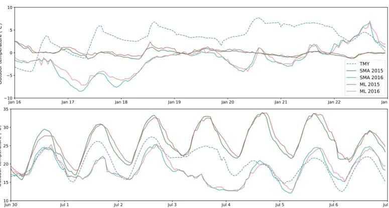
Figure2shows the temperature measured in the ML building compared to the measured temperature at the closest weather station (SMA) for a winter and a summer week in 2015 and 2016 along with the TMY data for the same weather station. The patterns observed on the summer week show hotter air temperatures in the on-site weather station

(8)

in the evenings as heat stored in the thermal mass of the buildings slowly gets released to the surrounding environment. The temperatures in the winter week show a lower daily variation than in summer, with the temperatures in the district almost always higher than in the SMA weather station. The minimum temperature in both years is lower for the SMA weather station than for the district, and the peak temperature in 2016 occurs on a different day for each sensor.

)()(

Figure 2.Measured temperature data from the off-site weather station SMA and from the on-site weather station ML for 2015 and 2016 compared to the typical meteorological year (TMY) data from the SMA weather station for a winter (top) and summer week (bottom).

The district’s energy demand was modeled using data from the SMA weather station and compared to results obtained when the outdoor temperature measured at the ML building was assumed as a climatic boundary condition. The energy demand results for each case were then passed on to the technology sizing and simulation tools in order to observe the effects on technologies’ costs and economic feasibility.

2.3. Solar Photovoltaic Potential

The CEA solar potential tool can be used to estimate the potential for photovoltaic (PV) panels, thermal collectors, and hybrid photovoltaic-thermal (PVT) collectors, both on roofs and walls. In this study, solar resources were only considered for electricity production, eliminating thermal collectors as an option. Preliminary results showed that the effect of occupant modeling on the performance of solar systems was similar for both PV and PVT, and thus only the former system is studied in this paper.

The solar technology potential tool first defines which surfaces receive enough solar irradiation throughout a year according to a user-defined irradiation threshold. The tool subsequently calculates the number of panels of a given size that can be placed in those areas by calculating the optimal tilt angle, row spacing, and surface azimuth of the panels on each surface. The tilt angle is calculated according to Quinn and Lehman [34]:

tanβ=cosγ·tanφ·

1+(τα)_d·g(kT)−(τα)_r·ρg

2·(1−g(k_T))

−1

(1)

(9)

whereγis the surface azimuth angle,φis the latitude,(τα)_dis the transmittance-absorptance product of the diffuse radiation (assumed equal to 0.98), (τα)_r is the transmittance- absorptance product of the reflected radiation (assumed equal to 0.97), and ρg is the ground reflectance.g(kT)is a function of the hourly clearness indexkT, defined as follows:

g(kT) =







0.97 forkT≤0.15,

1.237−1.361·kT for 0.15<kT≤0.7, 0.273 for 0.7<k_T.

(2)

whilek_Tis calculated from the mean daily diffuse radiation ¯T_{di f f}_,dailyobtained from the weather data:

kT=1−T^¯_{di f f}_,daily (3)

The row spacing of the panel arraysDis calculated in order to avoid panel shading during the winter solstice:

D= ^L·sinβ tanhS

·max[cos(π−γ), cos(γ−π)] (4) whereLis the module length andhSis the solar elevation at the winter solstice.

Given the panel size and row spacing, the maximum number of panels possible is installed on each surface that exceeds the predefined threshold. Based on the installed panel area calculated according to this methodology, the electricity produced is calculated following Osterwald’s method [35]:

Pel =η_NOCT·APV·S·^h1−Bre f·(Tcell−NOCT)ⁱ·lmisc (5) whereP_elis the electrical power output of a PV panel with an areaA_PV and an efficiency ofη_NOCTat the Nominal Operating Cell Temperature (NOCT) and a cell maximum power temperature coefficient ofB_{re f}as a function of the absorbed radiationSand cell temperature Tcellgiven miscellaneous losses oflmisc. As a simplifying assumption, CEA assumes a linear relationship between the temperature rise of solar panels and the absorbed radiation based on the operating condition at the NOCT [36].

The panels’ physical properties and nominal operating conditions are taken from the CEA technology database [30], whereas the absorbed radiation is calculated as a function of incoming radiation, thickness, refractive index, and extinction coefficient of the material [37]:

S= (τα)_n·M·

G_b·R_b·K_τα,b+G_d·K_τα,d· ¹+cosβ

2 +G·ρg·Kτα,g·¹−cosβ 2

(6) whereGis the incident solar irradiation,GbandGdare the beam and diffuse solar irradiation,(τα)_nis the incidence angle modifier for direct (beam) radiation,R_bis the ratio of beam radiation on a tilted surface to that on a horizontal surface,Mis an air mass modifier, Kτα,b = ^(τα)_(τα)^b

n is the incidence angle modifier at the beam incidence angle, andKτα,dand Kτα,gare the incidence angle modifiers at effective incidence angles for isotropic diffuse and ground-reflected radiation.

As a result, the tool produces the PV area installed in each façade and roof of each building as well as the hourly electricity production for each surface. In order to analyze the performance of solar technologies in the area for each occupancy model, the concepts of self-consumption and self-sufficiency are introduced. Self-consumption refers to the ratio between the electricity produced from PV that is consumed on site to the total electricity produced. Self-sufficiency, on the other hand, refers to the share of the electricity required that is produced on site. A change in the total electricity demand caused by an occupancy model will thus affect self-sufficiency, as the share of the total electricity demand that can

(10)

be covered by PV will be affected. On the other hand, if changes to occupancy patterns and occupant activities lead to a shift in energy demands between daytime and nighttime, the self-consumption will be increase or decrease as more or less electricity is consumed during daytime hours, when PV production is at its highest.

2.4. Thermal Network Modeling

For the analysis of district heating and cooling networks, CEA includes two different thermal models: a detailed model for the simulation of existing networks and specific designs, and a simplified model for the analysis of different network designs and for system optimization. Due to the long computational times required by the detailed thermal network model and the relatively small effects observed in an analysis of different scenarios for the case study district [38], for the present comparison the simplified thermal network model was used. In this model, the supply temperature is fixed at the highest or lowest temperature required from the network, depending on whether district heating or cooling is being modeled.

The hydraulic model is based on the Python package Water Network Tool for Re- silience (WNTR) [39]. The calculation procedure is similar to that of the detailed CEA thermal network model [38], save for the fact that the Hazen–Williams equation is used to calculate the pressure drop in each pipe instead of the Darcy–Weisbach equation. This is an appropriate assumption for water flowing in pipes, as is the case in the thermal networks considered here. The head loss in a pipeh_L(in meters) in WNTR is calculated as follows [40]:

hL= Hn_j−Hn_i =10.667·C^−1.852·d^−4.871·L·sign(q)· |q|^1.852 (7) whereCis the Hazen–Williams roughness coefficient (unitless),dis the pipe diameter (m), Lis the pipe length (m),qis the flow rate of water in the pipe (m³/s), andHn_j andHn_i are the heads at the starting node and at the ending node (m).

In CEA, the tool is first run in order to size the pipes in the network according to the mass flow rates required by each building’s substation. The pipe diameters obtained are then used as inputs to another run of the same simulation in order to calculate the pressure at each node and mass flow along each edge. Finally, the tool is run a third time in order to obtain the head losses at the plant node.

The thermal part of the detailed district network model in CEA involves iteratively calculating the network temperatures at each time step in order to ensure every consumer node is supplied the temperature required for its building systems. This iterative calculation leads to long computational times, which makes the tool impractical when comparing different network alternatives for a district. In the simplified tool, thermal losses are estimated by assuming the temperature of the network to be equal to the lowest temperature required by all buildings in the area for the given time step. Thus, for each pipe the inlet temperature is assumed to be equal to the required supply temperature and the outlet temperature of each pipe. Heat losses are then calculated using a resistance equivalency model:

Q˙ = ^∆T

R_pipe+R_insulation (8)

where ˙Qrepresents the thermal losses through the pipe,∆Tis the temperature difference between the fluid in the pipe and the ground, andR_iare the thermal resistances of the pipe and insulation material, calculated according to Wang et al. [41]. The thermal resistances of the ground and due to convection are neglected.

The thermal resistance of the pipe materialR_pipeand of the insulationR_insulationare calculated as a function of the interior and exterior diameter of the pipe or insulation layer (D_intandDext) and the thermal conductivity of the material (λ):

R_i = ¹ 2π·λ_i ·ln

Dext,i

D_int,i

,i∈I={pipe,insulation} (9)

(11)

Given the very simplified nature of the thermal calculation, the simplified model is not suitable for the detailed simulation of specific network designs, but is useful as a tool for network sizing and quick scenario comparison. For each case, a viable network layout was created by connecting all buildings in the case study through the minimum Steiner tree assuming pipes to be laid only in trenches in the existing street network. The thermal network is supplied by a centralized heating or cooling plant located at the building with the highest demand in the area. The performance of the resulting thermal network infrastructure is compared to a decentralized alternative, namely individual heat pumps and chillers installed in each building for heating and cooling, respectively.

3. Case Study

The effects of occupancy modeling and the urban heat island were tested on a case study in Zurich, Switzerland. The area hosts two universities (ETH Zurich and the Univer- sity of Zurich) and a hospital (the University Hospital of Zurich), as well as some minor secondary uses. Figure3shows each building’s main use type as well as the share of each building use type in the district’s total floor area.

Figure 3.Case study area showing the main function of each building (left) and the overall functional mix in the area (right), adapted from [26]. The location of the temperature sensor used for the analysis of urban climate is shown by a black cross on the ML building.

Office spaces include both university and doctors’ offices and are separated by their end users: ETH Zurich (ETH), University of Zurich (UZH), University Hospital Zurich (USZ), and others.

In order to construct the physical model of each building, building footprints were obtained from OpenStreetMap [42] and building heights were assigned based on the 3D model of the City of Zurich [43]. Basic information on each building, such as the main function, construction year, and heating systems, were obtained from the Swiss Federal Register of Buildings and Dwellings [44]. Wherever possible, these data were complemented with information obtained from the building owners to obtain detailed functional distributions and building systems. Window-to-wall ratios were estimated for each building, whereas building materials were taken from the CEA archetype database.

The complete set of inputs to the CEA demand model as well as the most important properties of each building in the case study area are shown in AppendixA.

The aim of this paper was to compare the effects of occupancy and climate assumptions on the planning of centralized and decentralized district energy systems in an urban area.

Thus, the precise modeling of the case study area’s existing district heating infrastructure or the proposed free cooling network [45] are beyond the scope of this analysis. In assessing the area’s PV potential, all available suitable roof and façade surfaces that exceeded the

(12)

minimum irradiation threshold of 800 kWh/m²/yr were assumed to be used for PV.

Monocrystalline PV panels with an efficiency of 18% were selected from the CEA technology database [30].

4. Results

4.1. District Energy Demand

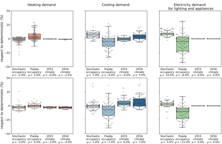
A full analysis of the effects of occupants and microclimate on the area’s demands is out of the scope of this paper and can be found in previous publications [20,28]. In this section, these effects are briefly summarized in order to help interpret the results obtained in the supply system sizing and simulation sections. Figure4shows the variation in the demands for heating, cooling, and electricity for lighting and appliances due to the different occupancy models and climate assumptions. The variation due to stochastic and PopAp occupancy modeling was calculated with respect to the standard deterministic schedules and TMY weather data. The deviation due to local climate is calculated by using local weather data from the ML building compared to the SMA weather station for the years 2015 and 2016.

− −

)()(

− − −

− − − −

−

Figure 4.Variation in the yearly and peak demands for heating, cooling, and electricity for lighting and appliances due to occupancy modeling and local climate. The horizontal lines in the box plots show the medians of the distributions, whereas the meanµof each is stated in the label for each case.

The PopAp results consistently showed a lower overall occupancy than the two standard-based approaches, as seen in Figure1. Since the electricity demand for appliances was correlated to the number of occupants in each building, the PopAp case also has the lowest demand for electricity. The lower number of occupants and decreased electricity demand also lead to a lower cooling and a higher heating demand compared to the deterministic baseline. The stochastic method, on the other hand, led to higher electricity demands and hence had an inverse effect on the heating and cooling demands. Due to the

(13)

higher variability in occupancy from one building to another, the PopAp case also leads to a larger spread in the distribution of the results, especially for electricity. Since the peak number of occupants in the stochastic case tends to approach that of the deterministic schedules, the deviation in the peak results is smaller than the yearly demands. For the PopAp case, on the other hand, the base number of occupants is very close to the other two approaches, but the peak is considerably lower. Thus, the effects on the peak demands for cooling and electricity are even greater.

The difference in the measured temperatures at the SMA weather station and at the ML building observed in Figure2also correspondingly leads to a change in the district’s energy demands. The yearly heating demand is barely affected by the difference in temperature between the district and the SMA weather station, whereas the peak heating demand variation is lower than 5% for all buildings. Due to the slightly higher outdoor temperature in the district, the heating demands are marginally lower for all buildings in the case study. For the cooling case, on the other hand, the difference is much more pronounced, with a variation in yearly demand of±6% for the year 2015 and−6 to+22% for 2016.

This difference is even more evident for the peak cooling power, which shows an average increase of 5–6% for each year with differences of more than 30% for individual buildings in both years. The electricity demand for lighting and appliances was naturally unchanged by the change in outdoor temperature.

Overall, both occupancy and outdoor temperature appear to have a more significant effect on the peak cooling than peak heating demand. Since the peak demand for heating is driven by the difference between outdoor and indoor temperature, the effects of the number of occupants or a small change in outdoor temperature have a much smaller effect.

For cooling, on the other hand, a change in outdoor temperature of 1 °C and changes in internal gains due to occupant presence contribute much more to the temperature difference that needs to be compensated by cooling systems, and hence the peaks are more strongly affected than the base loads.

4.2. PV Potential and Electricity Costs

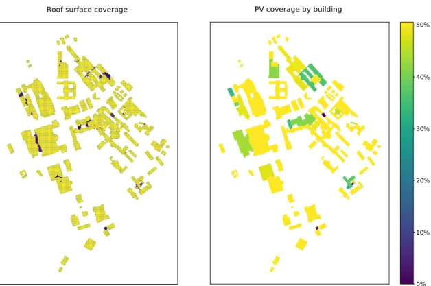
Given that CEA neglects roof shapes, most roof surfaces were found to be suitable for PV installation, and hence 97% of all roof areas were selected, as seen in Figure5.

Since panels are assumed to be placed at their optimal tilt angle and spaced accordingly, the area of PV installed per square meter of roof is much lower, with 49% coverage of all roof surfaces. This approach was found to give comparable results to a more detailed calculation accounting for roof tilt angles with a 100% roof coverage [46].

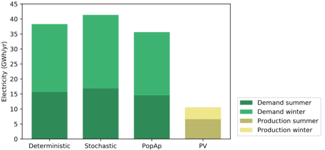
The performance of solar technologies in the area was assessed by looking at the self-consumption and self-sufficiency for each building. Figure6shows the distribution of these metrics for each occupancy model analyzed for all buildings in the area. The self- consumption for all occupancy models is relatively high, with an average rate of 74 to 77%. This is due on one hand to the high overall electricity demand in the area, which is much larger than the electricity obtained from PV both in summer and winter, as shown in Figure7. On the other hand, the buildings in the area, which are largely dominated by educational, research, and office functions, have a predominantly daytime occupancy, with only hospital rooms having nighttime occupancy. Therefore, most of the electricity demand occurs during times when PV production is at its peak.

The distribution is rather similar for all models, with self-consumptions ranging from 20 to 100%. This is due to the electricity demands for the individual buildings in the area being strongly dominated by process base loads and lighting, which were assumed to be independent of occupancy. The distribution for the stochastic case is shifted up due to the higher electricity demands for lighting and appliances predicted by this model.

The opposite trend can be observed regarding the self-sufficiency, which is inversely proportional to the demand. The PopAp case, having the lowest electricity demand, also leads to the highest self-sufficiency.

(14)

Figure 5.Roof surfaces selected for PV placement based on a minimum threshold of 800 kWh/m²/yr (left) and area of PV installed per unit area of roof surface for each building based on a minimum threshold of 800 kWh/m²/yr (right).

Figure 6.Distribution of the self-consumption and self-sufficiency of the installed PV for all buildings in the case study (top) and for education and office buildings (bottom) for each occupancy model.

(15)

()

Figure 7.Electricity demand for each scenario and photovoltaic (PV) production potential by season.

Education and office buildings were selected for further analysis as they provide a more generalizable case for the analysis of occupant modeling compared to the very specific needs of hospital functions. Indeed, in the absence of the very large base loads in the hospital buildings, the self-consumption decreases and the self-sufficiency increases on average. The general trends observed in the distributions and relative values for different occupant models, however, remain the same, with the stochastic case having the highest self-consumption and the PopAp case the highest self-sufficiency.

At the individual building scale (Figure8), an average variation in the self-sufficiencies due to the occupancy model of±2% can be observed. A maximum deviation of−10–18%

is observed for one outlier, corresponding to a very small building. Similar variations can be observed in the self-consumption (±2%) with a maximum deviation of−10–5% for the same small building.

0 20 40 60 80 100

Buildings

0%

20%

40%

60%

80%

100%

Self-consumption

0 20 40 60 80 100

Buildings

0%

20%

40%

60%

80%

100%

Self-sufficiency

GymHospital LabLibrary Museum Office Restaurant School

Figure 8.Range of self-consumption (top) and self-sufficiency (bottom) for each building for different building use types.

The range of variation caused by the different occupancy models is shown as the black error bars for individual buildings.

(16)

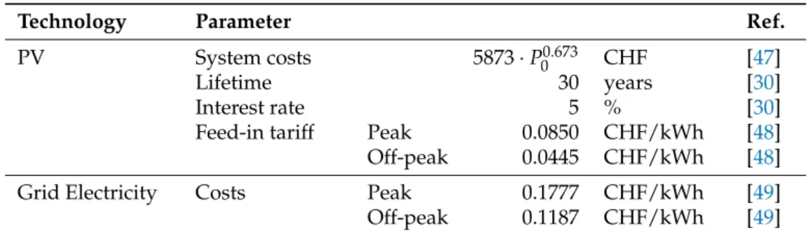
The effects of the occupancy models on the electricity costs in the area are analyzed for the case with photovoltaic panels as well as for the case where electricity is taken directly from the grid. The peak and off-peak costs of electricity for large-scale, medium-voltage consumers and feed-in tariffs from the local utility were assumed. The cost of photovoltaic systems was obtained by fitting an exponential curve to a dataset of sample costs for the Swiss context [47], as shown in Table2. The investment costs for the PV systems are compared by their total annualized costs (TAC), comprising the operational expenditures (OPEX) and annualized capital expenditures (CAPEXa):

TAC=OPEX+CAPEXa =OPEXa+C_inv· ^r·(1+r)^τ

(1+r)^τ−1 (10) whereCinvare the investment costs,ris the interest rate of the technology, andτis the lifespan of the technology.

Table 2.Installation and operation costs assumed for the grid electricity and photovoltaic panels.P0

is the peak power of the PV system, in kW.

Technology Parameter Ref.

PV System costs 5873·P₀^0.673 CHF [47]

Lifetime 30 years [30]

Interest rate 5 % [30]

Feed-in tariff Peak 0.0850 CHF/kWh [48]

Off-peak 0.0445 CHF/kWh [48]

Grid Electricity Costs Peak 0.1777 CHF/kWh [49]

Off-peak 0.1187 CHF/kWh [49]

For all scenarios, the implementation of PV in the area at the scale considered leads to a 10% decrease in the total annualized costs of electricity. Due to the different yearly demands produced by each model (Figure7), there is a change in the electricity costs of

±7.5% for the stochastic and PopAp models with respect to the deterministic baseline, whereas for the case of PV the difference is±8%.

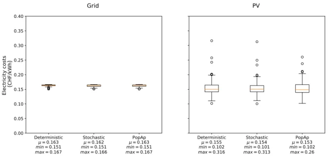
Since the costs of electricity change between peak and off-peak times, the costs per unit of electricity consumed by each building in the area (Figure9) give insight into the effect of occupancy on the dynamics of electricity consumption. The costs for the case where no PV was installed proved to be nearly the same for all buildings due to the predominantly daytime occupancy of all buildings in the area. Since most electricity consumption for all occupancy models occurs during peak times (6:00 to 22:00 Monday through Saturday), there is no significant load shift towards off-peak hours, and hence the costs are relatively constant.

The difference in costs is somewhat more pronounced for the case with PV, where the PopAp case has the lowest electricity costs on average. This is due to the fact that this model predicted the lowest electricity demand, and hence less electricity needs to be purchased from the electricity grid. A number of outliers in the plot correspond to buildings with oversized roof installations and relatively low electricity demands. These buildings would be good candidates to connect with surrounding buildings with large demands in order to further increase the self-consumption of photovoltaic systems in the area, and thus reduce the operational costs.

(17)

()

Figure 9.Distribution of the costs per kWh of electricity consumed by the buildings in the district for each of the occupancy models assuming PV is installed compared to when all electricity comes from the grid.

4.3. Heating and Cooling System Sizing and Costs

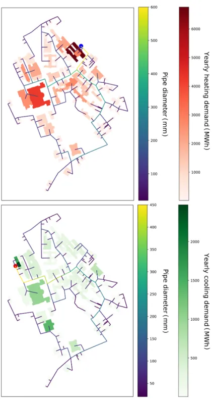
The district heating and cooling networks obtained by connecting all buildings in the case study through the minimum Steiner tree through the existing street network are shown in Figure10. The area has a large base load in a building that houses a large server room, where the cooling plant is also assumed to be located. In the heating case, the plant is located in a hospital building with a high process heating base load.

The thermal networks are assessed by comparison to a decentralized option. For the decentralized cooling case, individual chillers installed in every building with a cooling demand were considered. For the heating case, heat pumps were assumed to be used for both the centralized and decentralized cases, based on the expectation that supply systems will be increasingly electrified in the future. For simplicity, air-source heat pumps were assumed for both cases since access to geothermal in the area is limited, and the COP for these systems was calculated based on the required supply temperature and outdoor air temperature for all cases. While the temperature levels required by the building stock in the area are relatively high (assumed at around 70 °C), a large number of buildings in the area was indeed served by a district heating network fed by a water-source heat pump until 2017. Thus, while the system used for this comparison has a low COP, and indeed is in the process of being replaced by a higher efficiency energy concept [50], it has been demonstrated to be technically feasible. While thermal networks were modeled in detail, chillers and heat pumps were not explicitly modeled. Instead, only their demand for electricity was considered by calculating a dynamic COP for each system.

(18)

( ) ( )

Figure 10.District heating (top) and cooling (bottom) network layouts produced for the deterministic occupancy model along with the cooling loads for each building in the area. The location of the cooling plant is indicated by a blue and a red dot, respectively. The same layout was used for the two other occupancy models and weather cases, although some of the pipe sizes were different.

The costs of each heating and cooling system alternative were calculated according to the CEA database, as summarized in Table3. For the decentralized case, only heat pump and chiller costs were considered. The centralized option comprises centralized heat pumps or chillers, a thermal network, and a heat exchanger at each substation. Pump costs were negligible and were thus not considered. The piping costs of the thermal network depend on the nominal diameter of each pipe, which for the thermal networks in this case study ranged between DN20 and DN600.

(19)

Table 3.Investment costs, lifetime, and interest rates assumed for thermal networks and heating and cooling systems [30].P₀is the design capacity of the system, equal to the peak power required in kW.

Technology Parameter

Chillers Costs 361·P₀ CHF

Lifetime 25 years

Interest rate 5 %

Heat pumps Costs 197.2·P₀^0.49 CHF

Lifetime 25 years

Interest rate 5 %

Thermal network Costs by size DN20–DN600 492–5562 CHF/m

Lifetime 50 years

Interest rate 5 %

Heat exchangers Costs by size 50–80 kW 69.65·P₀−346.2 CHF

80–100 kW 5198 CHF

>100 kW 83.16·P₀−3118.5 CHF

Lifetime 20 years

Interest rate 5 %

4.3.1. Effects of Occupancy

Given the lower electricity demands observed for the PopAp case (Figure7), the internal gains in this scenario are also lower, and hence the overall cooling demand is also the lowest for this case. As a result, this method has an overall smaller pipe size distribution than the other two methods (Figure11). The backbone of the network is also noticeably smaller for this occupancy model than for the others, with fewer pipes of diameter 450 mm for the PopAp case compared to the other two models. Contrary to the results for space cooling, the stochastic model leads to the lowest predicted heating demand. Correspond- ingly, the pipe size distribution shows the stochastic model also required smaller pipe sizes.

However, given that the relative change in yearly demand between models is not as large as for the cooling case (71–76 GWh/yr, as seen in Figure12), the larger pipes that serve as the backbone to the district heating network have the same size for all occupancy models.

Figure 11.Number of pipes of each nominal diameter for the district heating (left) and cooling (right) networks produced for each occupancy model.

The energy demand required to operate the district heating network is also very similar for all cases, though it is 1–2% smaller for the PopAp case than the others. For both the heating and cooling cases (seen in Figures12and13), the yearly pumping electricity and thermal losses are marginal compared to the heating and cooling demands in the buildings for all cases. The district cooling network operation energy roughly follows the cooling

(20)

demand, being highest for the stochastic occupancy model, which has a demand 3.5 to 7.5%

higher than the other two models. The same pattern can be observed regarding the peak cooling and network operation demands, although in this case the peak pumping energy demand is higher than the peak thermal losses. The same general trends can be observed for the peak heating demand and peak thermal losses in the district heating network.

( ) ( )

Figure 12.Yearly (left) and peak (right) heating demand, and pumping electricity and thermal losses in the district heating network for each occupancy model.

By connecting the buildings to a thermal network, the peak demand of the entire district is lower than the decentralized case. However, compared to the findings from a previous analysis of a lake water district cooling network in the area [38], the electricity demand for operating the pumps in the network is particularly low. This is due in part to the fact that in this case the network is assumed to be supplied by local chillers, and hence there is no need to transport large volumes of water from the lake in order to provide free cooling. Furthermore, given that only research and hospital buildings are considered in this paper, there are much fewer buildings with low demands, which were found to lead to considerable pressure losses. Finally, the server room in the area had not been considered in the previous study, and hence the base load of the district cooling system was much lower.

( ) ( )

Figure 13.Yearly (left) and peak (right) cooling demand, and pumping electricity and thermal losses in the district cooling network for each occupancy model.

The resulting TAC for each heating alternative, shown in Figure14, show that the choice of occupant model can have a noticeable impact on the systems selected in each case. The centralized solution was found to be preferable when the deterministic and stochastic occupancy models were used, whereas the decentralized alternative was more

(21)

cost-effective for the PopAp case. Overall, the choice of occupant model was found to cause the total annualized costs of the centralized system to vary by±5% as opposed to

±3% for the decentralized case.

Regarding the cooling system alternatives, the PopAp case leads to 4% lower investment costs for the thermal network than for the other two models due to its comparatively smaller pipe sizes. The lower peak cooling power also leads to 10–13% lower chiller costs for this case, both for the centralized and decentralized alternatives. The stochastic model, on the other hand, leads to the biggest investment costs for both alternatives, but only about 1% higher than the deterministic model. Regardless of system alternative, the PopAp case leads to the lowest operational costs and the stochastic model the highest, with an overall range of−6–4% of the costs according to the deterministic method. Overall, the decentralized systems always had lower annualized costs (1.89 million CHF/year on average) compared to the district cooling network (2.16 million CHF/year). For both systems, the choice of occupancy model was found to lead to a±5% variation in TAC.

( )( )

Figure 14. Total annualized costs for the centralized (C) and decentralized (D) heating (top) and cooling (bottom) alternatives for each occupancy model.

4.3.2. Effects of Outdoor Temperature

The effects of the use of local weather data on supply system sizing was again tested by comparing centralized and decentralized heating and cooling systems for each of the weather scenarios observed. There is a noticeably smaller backbone in the district cooling network for the cases using 2016 weather data due to the overall lower cooling demands in that year. This can be seen in the pipe size distribution (Figure15), which shows that for the district cooling network sized according to 2016 weather data the maximum pipe size is DN400 as opposed to DN450 for all other cases. The difference in sizing due to different outdoor temperature assumptions is rather minimal by comparison, however, with minimal differences in pipe sizes for the SMA and ML cases for each year. In the heating case, where the differences in yearly and peak demands were found to be smaller,

(22)

there is a much smaller variation in pipe sizes, especially for the backbone of each thermal network. For smaller pipe diameters, which are sized to supply end consumers, there is somewhat more of a difference, with the network sized according to 2016 weather data again having a larger number of smaller pipes compared to all other cases.

Figure 15.Pipe diameter distribution for the district heating (left) and district cooling network (right) for each weather scenario.

Due to the differences in demand created by the weather data for the years 2015 and 2016, the total annualized costs of the cooling system alternatives vary widely when sizing according to different weather cases (Figure16). For both cooling systems, the costs are highest when using 2015 weather data due to a heat wave that took place that summer, whereas the lowest costs are obtained when using 2016 weather data. This point illustrates why systems are typically sized using TMY weather data rather than individual years’

measurements. In this case, however, the comparison of sizing results for individual years provides an estimate for the uncertainty introduced by the use of weather station data on system sizing.

Since a linear relationship between chiller costs and design capacity was assumed (as shown in Table3), the deviation in the peak cooling power by year observed in Figure4 correspondingly leads to a deviation in chiller costs for individual buildings between−7.5 and 43.5%. This points to a considerable uncertainty in system sizing due to the effects of local climate. The capital expenditures for the entire district increase by between 5 and 7%

for the decentralized alternative when sizing according to the local measurements from the ML building, whereas this increase is somewhat smaller for the centralized system (3–4%

higher costs). The operating expenses, on the other hand, vary by−0.6–2.1% due to the use of local temperature data.

The TAC for both heating alternatives for each weather scenario are shown in Figure16.

The variation in costs for the different weather cases is relatively minor compared to the cooling case. The system costs when sizing according to TMY data are again presented for reference, as these are sized to meet the demands of a “typical” year. Regarding the deviation in costs caused by the local climate, the use of temperature data from the ML building leads to a 3–4% increase in the investment costs and an increase in the operation costs of less than 1% for the centralized case. For the decentralized alternative, a similar trend can be observed in the operation costs, but the investment costs are about 1% lower.

(23)

( )( )

Figure 16. Total annualized costs for the centralized (C) and decentralized (D) heating (top) and cooling (bottom) alternatives for each weather scenario.

5. Discussion

5.1. Occupant Effects on PV Performance and Electricity Costs

As observed in the previous sections, the choice of occupant model appears to have a considerable impact on the yearly electricity demand of the area. The demand for electricity is higher for the deterministic and stochastic methods than the PopAp case. The reason for this is that the latter approaches show a higher number of occupants in the district, and consequently the electricity demand for appliances is also higher. This is consistent with previous studies [51–53] that found that building standards tend to overpredict the number of building occupants at a given time.

Given the particular characteristics of this area, however, the electricity demands are largely driven by lighting and processes, which were assumed to be independent of occupant presence. Hence, the self-consumption of the PV installation analyzed was found to be high for all cases. In spite of the low electricity prices available to large-scale consumers such as the three institutions that occupy this area, the self consumption was found to be high enough to make PV economically viable for all occupant models.

It could therefore be tempting to conclude that simplified occupant modeling approaches are sufficient for the planning of photovoltaic systems. However, this might not be the case in areas with a lower share of process energy demand and where occupants’

actions have a more direct impact on the total electricity demand. Likewise, in this specific case study the lighting demand was not affected by occupants, but in other cases occupants’

activities and their associated electricity demands might have a larger impact on electricity demand and PV performance.

As mentioned in the introduction, the ability to accurately estimate occupant presence patterns appears to be the main driver for reliable estimations of annual heating, cooling, and lighting demand in buildings [17]. Assuming that the PopAp case, being the only data-driven approach under consideration, represents reality more closely, the other two

(24)

models would appear to overestimate the electricity demands of the area. When planning photovoltaic systems, the use of the stochastic model would thus lead to an overly opti- mistic estimate of the self-consumption in the area. However, due to the higher amount of electricity that needs to be purchased from the grid, the average electricity costs for this scenario would also be overpredicted.

5.2. Effects of Occupant Presence and Outdoor Temperature on Thermal System Sizing and Costs The choice of occupancy model and climatic boundary conditions were found to have a direct impact on the heating and cooling demands of the district and thus affect the sizing of both the centralized and decentralized alternatives considered.

As observed in the previous sections, most noticeably for the population-based approach in the cooling case, the choice of occupancy model can have an impact on the thermal network sizing and hence on the cost of the centralized system alternative. The choice of occupancy model was thus found to affect the costs of implementing thermal networks in the area by a margin of±5%. The use of local temperature data, on the other hand, led to an increase in the TAC for both the district heating (3–4%) and cooling infrastructure (4–9%). Comparing centralized and decentralized alternatives, the variation in annualized cooling costs was not significant enough to make a difference in the choice of systems at the district scale, since the decentralized alternative was found to be more cost-effective for all cases. In the heating case, on the other hand, the variation in the costs of the supply system alternatives was smaller, and thus the choice of occupant modeling approach was significant enough to affect the feasibility of the district heating infrastructure.

Regarding the effect of occupant modeling on the decentralized system alternatives, while the difference in total annualized costs for the entire district was±5% for the cooling case and±3% for the heating case, the variation for individual buildings is much larger, as seen in Figure17. For the heating case, only two buildings showed changes in total annualized costs greater than±10%, and these buildings had relatively small demands.

For the cooling case, the small variation observed on the district scale might be strongly influenced by the small relative variation of the three outlier buildings in the area (which correspond to a building complex that houses a server room and thus has much higher demands than any other building in the area). However, 30 buildings of all demand ranges out of the 104 buildings in the area were found to have variations in the TAC of at least

±10%, meaning that the choice of occupancy model can have a considerable impact on the choice of cooling systems for individual buildings. The effect of local climate on the sizing of cooling systems was even more pronounced, with a variation of more than 20%

for a number of buildings. This stresses the effect of the urban heat island on the cooling demands of urban areas, and thus the cooling costs.

Given the preceding observations, it appears that both the choice of occupancy model and climatic boundary conditions used can have a considerable impact on the cost of system alternatives. In particular, these modeling choices have a much more significant effect on the planning of cooling systems. This effect is most clearly observed in the single building scale, which might explain why there has been a number of increasingly detailed approaches for occupancy and microclimate modeling at this scale compared to the relatively simplified methods used at the urban scale, as discussed in the introduction and observed in the literature [16,54]. However, since occupancy was found to be significant enough to affect the sizing and cost performance of thermal networks, work should continue to be carried out on the development of district-scale occupancy models that are generalizable enough to be applied in the planning of district-scale energy systems in other contexts.

An important limitation in the present analysis is that each of these energy systems was considered separately rather than as an overall integrated system. The PopAp case, for example, was found to have the lowest electricity demand, which led to the highest self-consumption of locally-produced electricity and thus the lowest electricity costs. This decrease in electricity demand however also led to lower cooling demands and higher heating demands, meaning that for electrified thermal supply systems such as the ones

(25)

analyzed here there would be a higher demand in the cold season, when photovoltaic production is lowest. Thus, if the electricity demands arising from heating and cooling supply were to be considered along with the solar systems, the occupancy models might affect the economic viability of PV in a different way.

( )( )

Figure 17.Average total annualized costs per square meter for the decentralized heating (top) and cooling (bottom) systems for each building in the area along with the minimum and maximum costs caused by the choice of occupancy model.

Buildings with a variation greater than±10% are marked in dark red (heating) and dark blue (cooling).

6. Conclusions

Comparing the sizing and costs of energy supply systems under different occupancy models and climatic boundary conditions allowed us to observe the effects these stochastic sources of uncertainty have on the performance and costs of energy systems at both the district and building scales. For the case study in question, the effects of building occupants on the costs of electricity, heating, and cooling for the selected reference district-scale systems were quantified at±8%,±5% and±5%, respectively. Likewise, the change in temperature due to the urban heat island led to an increase in the total annualized costs of up to 4%. As expected, however, these effects were much more sizable for individual buildings, for which the cooling demand varied by as much as 22% due to this increase in temperature.

The detailed assessment of building occupants and the local microclimate therefore appears a necessary step at the building scale, given that their effects can lead to significant sizing errors. When scaling up to the district scale, on the other hand, individual peaks are aggregated, leading to a much smoother load curve and hence less variation due to these stochastic sources of uncertainty. It could therefore be tempting to conclude that one can simply apply simpler, tried, and tested methods and assume any localized variations will be averaged out on the aggregate. However, the variation caused by these sources of uncertainty was found to be significant enough to affect the decision on the more cost- effective heating alternative for both occupancy and outdoor temperature. Thus, errors at this scale could lock an entire district into sub-optimal supply systems.

Author Contributions: Conceptualization, review and editing, M.M.-R. and A.S.; methodology, model development, formal analysis, data curation, visualization, and original draft preparation,