Over the Last 32,000 Years

Atmospheric CO

₂

Over the Last 32,000 Years

Thomas A. Ronge¹ , Matthias Prange² , Gesine Mollenhauer¹ , Maret Ellinghausen², Gerhard Kuhn¹ , and Ralf Tiedemann^1,2

1Department of Marine Geology, Alfred‐Wegener‐Institut Helmholtz‐Zentrum für Polar‐und Meeresforschung, Bremerhaven, Germany,²MARUM Center for Marine Environmental Sciences, Universität Bremen, Bremen, Germany

Abstract

It is widely assumed that the ventilation of the Southern Ocean played a crucial role in driving glacial‐interglacial atmospheric CO2levels. So far, however, ventilation records from the Indian sector of the Southern Ocean are widely missing. Here we present reconstructions of water residence times (depicted asΔΔ¹⁴C andΔδ¹³C) for the last 32,000 years on sediment records from the Kerguelen Plateau and the Conrad Rise (~570‐to 2,500‐m water depth), along with simulated changes in ocean stratification from a transient climate model experiment. Our data indicate that Circumpolar Deep Waters in the Indian Ocean were part of the glacial carbon pool. At our sites, close to or bathed by upwelling deep waters, wefind two pulses of decreasingΔΔ¹⁴C andδ¹³C values (~21–17 ka; ~15–12 ka). Both transient pulses precede a similar pattern in downstream intermediate waters in the tropical Indian Ocean as well as rising

atmospheric CO2values. Thesefindings suggest that¹⁴C‐depleted, CO2‐rich Circumpolar Deep Water from the Indian Ocean contributed to the rise in atmospheric CO2during Heinrich Stadial 1 and also the Younger Dryas and that the southern Indian Ocean acted as a gateway for sequestered carbon to the atmosphere and tropical intermediate waters.

Plain Language Summary

By analyzing air bubbles trapped in glacial ice from Antarctica, we know the pattern of atmospheric CO2for roughly the last 800,000 years. This record shows a distinctive pattern of warm interglacials with high values of atmospheric CO2(~280 ppm) and cold glacials with CO2as low as ~180 ppm. A leading hypothesis assumes that the CO2that went“missing”from the atmosphere during the glacials was stored in the deep global ocean. Several studies suggest that during glacials, the main connection between the deep ocean and the surface/atmosphere—the Southern Ocean—was significantly interrupted or at least reduced. Until now, it was shown that the deglacial South Pacific, the Drake Passage, and the South Atlantic played a vital role in the release of the stored oceanic CO2back to the atmosphere. With our study, we want to shed new light on the role, the southernmost Indian Ocean played in this system. Our data from the Kerguelen Plateau and the Conrad Rise indicate that the Indian Ocean also stored CO2during the last glacial and released it back to the atmosphere in two pulses during the last deglacial transition.

1. Introduction

The reconstruction of glacial and interglacial CO2‐cycling is fundamental to our understanding of the pre- sent and future global carbon cycle. At the end of the last glacial, the 90 ppm rise in atmospheric CO2

(Marcott et al., 2014) was linked to a significant 190‰drop in atmospheric radiocarbon activities (Δ¹⁴C;

Broecker & Barker, 2007; Reimer et al., 2013). The covariation of atmospheric CO₂andΔ¹⁴C implies a pro- cess acting upon both patterns. As this 190‰decrease cannot be explained by the atmospheric formation of

14C (Broecker, 2009; Broecker & Barker, 2007; Butzin et al., 2012; Laj et al., 2002; Reimer et al., 2013), the release of old, and therefore ¹⁴C‐depleted CO2 from a large carbon reservoir such as permafrost soils (Köhler et al., 2014; Winterfeld et al., 2018) and/or the deep ocean (Burke and Robinson, 2012; Ronge et al., 2016; Skinner et al., 2010; Skinner et al., 2015) is considered the most likely driver. The sequestration of carbon (CO₂) within the deeper ocean would require a major climate‐response of polar upwelling regions and thus significant changes in global deep water circulation (Sigman et al., 2010). Several sediment and

©2020 The Authors.

This is an open access article under the terms of the Creative Commons Attribution‐NonCommercial License, which permits use, distribution and reproduction in any medium, provided the original work is properly cited and is not used for commercial purposes.

Key Points:

• Glacia‐interglacial circulation of the Indian sector of the Southern Ocean

• Indian Ocean part of glacial oceanic carbon pool

• Southern Indian Ocean was source of CO₂during Heinrich Stadial 1 and during the Younger Dryas

Supporting Information:

•Supporting Information S1

•Figure S1

•Figure S2

•Figure S3

•Figure S4

•Figure S5

•Figure S6

Correspondence to:

T. A. Ronge, thomas.ronge@awi.de

Citation:

Ronge, T. A., Prange, M., Mollenhauer, G., Ellinghausen, M., Kuhn, G., &

Tiedemann, R. (2020). Radiocarbon evidence for the contribution of the Southern Indian Ocean to the evolution of atmospheric CO2over the last 32,000 years.Paleoceanography and Paleoclimatology,35, e2019PA003733.

https://doi.org/10.1029/2019PA003733

Received 24 SEP 2019 Accepted 24 FEB 2020

Accepted article online 27 FEB 2020 Classification:Physical Sciences– Earth, Atmospheric and Planetary Sciences

coral records from the Atlantic and the Pacific Oceans point to increased aging of deep glacial water masses (below ~2,000‐m water depth) or to increased deglacial ocean‐atmosphere interaction, via the Southern Ocean (Burke & Robinson, 2012; Burke et al., 2015; Cook & Keigwin, 2015; Ronge et al., 2016; Sikes et al., 2016; Sikes et al., 2000; Skinner et al., 2010; Skinner et al., 2015). On the other hand, several other studies fail to record any significant aging of glacial deep waters (e.g., Broecker et al., 2004/Broecker et al., 2008;

Broecker & Clark, 2010; Lund et al., 2011; Zhao et al., 2018). These discrepancies further stress the impor- tance of research in thisfield, highlighting the importance of our new South Indian Ocean data. In the con- text of deep water‐to‐atmosphere circulation and interaction, the Southern Ocean in particular plays a key role. Today, up to 65% of all deep water masses upwell around Antarctica to make theirfirst contact with the atmosphere (DeVries & Primeau, 2010). Within the Southern Ocean, the amount of upwelled deep waters (Marshall & Speer, 2012) and their surface residence time and the biological primary productivity (Studer et al., 2015) are important factors, controlling the amount of released or sequestered CO2. To allow for the sequestration of CO₂within the ocean, upwelling of deep waters must have been reduced or even shut down during glacial times, most likely in combination with expanded sea ice. Evidence for the existence of carbon‐enriched old deep waters has been found within the deep glacial South Atlantic Ocean (Skinner et al., 2010), the Drake Passage (Burke & Robinson, 2012; Chen et al., 2015; Rae et al., 2018), the South Pacific (Ronge et al., 2016; Siani et al., 2013; Sikes et al., 2016; Skinner et al., 2015), and in southern sourced Intermediate Waters (Bryan et al., 2010; Marchitto et al., 2007). However, geological sources of¹⁴C‐dead car- bon, such as hydrothermal vents or decaying clathrates, are important processes that have to be considered, when analyzing and interpreting marine radiocarbon records (e.g., Stott et al., 2009/2019; Ronge et al., 2016).

One link, the Indian sector of the Southern Ocean, is largely missing to provide a comprehensive picture of Southern Ocean water mass ventilation and radiocarbon inventories during glacial stages and the outgassing history throughout deglacial transitions, with associated reconfigurations of the Southern Hemisphere Westerly Winds and the Antarctic Circumpolar Current (ACC) system (Buizert et al., 2018; Katsuki et al., 2012; Menviel et al., 2018; Oiwane et al., 2014; Sime et al., 2013).

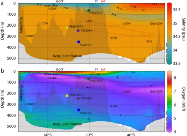
Here, in order tofill this knowledge gap, we present radiocarbon data from three sediment records from the Kerguelen Plateau and the Conrad Rise (Figure 1; Orsi et al., 1995). These records cover the ventilation his- tory of the Indian branch of Upper and Lower Circumpolar Deep Water (UCDW/LCDW) from 567 to 2,545 m water depth (Figure 2; Garcia et al., 2014; Locarnini et al., 2013; Schlitzer, 2019). As it is shown in Figure 2, the combination of these records enables us to reconstruct the ventilation history of old, carbon‐rich, deep waters on their way south toward the Antarctic upwelling regions, as well as their pathway toward the sur- face prior to the process of air‐sea gas exchange and the formation of northbound intermediate waters.

Furthermore, a returnflow of southern bound Indian Deep Water (IDW) is feeding the UCDW of this sector.

Like in the Pacific Ocean, this modern IDW consists of old, carbon‐rich waters, which are ultimately fed into the circumpolar system. Corresponding to Ronge et al. (2016), we assume that the glacial counterpart of modern IDW was an integral part of the glacial mid‐depth carbon pool. Ultimately, we conclude that the Indian sector of the Southern Ocean was an important part of the global deep water carbon pool that must not be neglected in reconstructions and modeling studies investigating the global carbon cycle.

1.1. Regional Oceanography

In the Indian sector of the Southern Ocean, the Conrad Rise (52°S–54°S; 39°E–47°E) marks a considerable obstruction to the bottom reaching ACC (Ansorge et al., 2008). The shallow Conrad Rise forces the ACC to bifurcate, forming two distinctive jets, surrounding the obstruction (Durgadoo et al., 2008). On its circumpo- lar journey, the ACC is faced with another major topographical feature, the Kerguelen Plateau, located between 46°S and 64°S (Figure 1). While the major part of the ACC, with up to 100 Sverdrup is deflected toward the north of the plateau (Park et al., 1991; Park et al., 1995) about 40 Sverdrupflow around the south and continue their eastward directedflow path between the Kerguelen archipelago and Antarctica (Park et al., 2008). North of the Kerguelen Islands, the Subantarctic Front sits at about 45°S (Figures 1 and 2), in close proximity to the Subtropical Front ~2° to the north (Park & Vivier, 2011). On the plateau, below the surface mixed layer, the remnants of the last winter mixed layer (Park et al., 1998), the so‐called Winter Water (WW), occupy the water depth from ~70 to 400 m with a maximum of about 700 m (Park et al., 2008). The northernmost extent of WW is by some authors also considered to be the location of the Antarctic Polar Front (APF; Park & Vivier, 2011). Park and Vivier (2011) derive the APF position from the

subsurface minimum colder than 2°C and locate the position directly south of the Kerguelen Islands.

However, other studies (Dezileau et al., 2000; Johnson, 2007) locate the APF to the north of the archipelago. As the World Ocean Atlas 13 Data (Locarnini et al., 2013) show <2°C subsurface waters to the north, we follow the latter authors and place the APF to the north of the Kerguelen archipelago (Figures 1 and 2). Therefore, the Southern ACC Front coincides with the northern WW limit with subsurface temperatures of 0°C south of the main archipelago (Figures 1 and 2; Park et al., 2009). Below the WW, UCDW is characterized by a prominent oxygen minimum and a temperature and nutrient (phosphate) maximum between 400 and ~1,400 m (Garcia et al., 2014; Locarnini et al., 2013; Park et al., 2008; van Beek et al., 2008). Further down, a salinity maximum marks LCDW from 1,400 to 2,600 m, while Antarctic Bottom Water can be distinguished by increasing oxygen but decreasing salinity and temperature values below 2,600‐m water depth (Garcia et al., 2014; Locarnini et al., 2013; Park et al., 2008; van Beek et al., 2008). Below a depth of about 4,000 m, Antarctic Bottom Water becomes the dominant water mass, circulating in a clockwise manner around the plateau (Dezileau et al., 2000).

2. Methods

Our reconstructions are based on five sediment cores from the Indian Sector of the Southern Ocean (Figure 1). On the Conrad Rise, PS2606‐6 (S53°13′53.976″E40°48′5.976″) and PS2620‐3 (S50°41′6″E40°7′ 59.988″) were recovered in water depths of 2,545 and 3,593 m, respectively. Further to the east, PS69/912‐3 and PS69/912‐4 (S50°18′37.8″E71°34′3.576″; 567 m) and PS69/907‐2 (S55°0′14.976″E73°20′ 2.4″; 2253 m) were recovered on the Kerguelen Plateau (Figure 1).

2.1. Radiocarbon Analyses

For the reconstruction of the evolution of water mass ventilation, we analyzed paired samples of planktic (Neogloboquadrina pachyderma or mixed planktics) and mixed benthic (Uvigerina peregrina and Figure 1.Map of the research area. The colored dots represent the sediment cores; the red line represents the Subantarctic Front; the blue line represents the Antarctic Polar Front; the black line represents the South Antarctic Circumpolar Current Front; the white lines represent the sections used in Figures 2 (I), 6a (II), and 6b (III). Frontal systems according to Orsi et al. (1995). Map created using GeoMapApp.

Cibicidoidesspp.) foraminifers. Paying attention that no broken, discolored, orfilled tests were picked, the samples were measured at the NOSAMS (National Ocean Science Accelerator Mass Spectrometer) facility in Woods Hole, USA, as well as the MICADAS (Mini Carbon Dating System) facility at the Alfred‐ Wegener‐Institute in Bremerhaven, Germany. At the latter, samples were analyzed as gas targets and con- tained 100μg C or less. Based on samples proximal to our research area, a recent study highlighted the relia- bility and significance of the MICADAS gas method (Gottschalk et al., 2018).

Raw planktic¹⁴C‐ages were converted into calendar ages, using the Calib7.1 software (Stuiver et al., 2018) along with the INTCAL13 calibration curve (Reimer et al., 2013). For the calibration, we used modeled sur- face reservoir ages proposed by Butzin et al. (2017; Figure S1 in the supporting information). This model simulates reservoir age changes at a similar latitude in the Southwest Pacific within a deviation of about 30 to 300 years to reconstructed surface reservoir ages (Skinner et al., 2015).

To select the most plausible modeled surface reservoir ages, we correlated the X‐rayfluorescence (XRF)‐ based Fe‐records of sediment cores PS2610‐3 and PS69/907‐2 to the dustflux record of the EDC ice core in afirst step (Figure S2; Lambert et al., 2008). Achieving a good correlation, we subsequently tuned the Fe‐records of PS69/912 to PS69/907‐2 and PS2606‐6 to PS2610‐3, respectively (Figure S2). Thisfirst age assignment already resulted in a good agreement of the distribution of raw¹⁴C‐ages (Figure S2) and served as the baseline to select the surface reservoir ages in the Butzin et al. (2017) model.

Ultimately,¹⁴C ages were converted intoΔ¹⁴C‐values in accordance to the method of Adkins and Boyle (1997). Using the calibrated¹⁴C‐ages from the planktic foraminifera, we then calculated the deep water to atmosphereΔ¹⁴C‐offset (ΔΔ¹⁴C) as the difference between the deep waterΔ¹⁴C and the IntCal13 reference curve (Reimer et al., 2013).

Figure 2.Cross section I, as indicated in Figure 1. (a) Salinity (Zweng et al., 2013) and (b) oxygen (Garcia et al., 2014). UCDW/LCDW: Upper/Lower Circumpolar Deep Water; AABW: Antarctic Bottom Water; IDW/CDW; Indian/Circumpolar Deep Water; frontal systems as indicated in Figure 1. Sections generated using ODV (Schlitzer, 2019); color‐scheme (A)Darjeeling Limitedby Patrick Rafter (https://prafter.com/color/). Shading represents the GEBCO_2014 bathymetry (Weatherall et al., 2015). PS2606‐6 and PS2610‐3 projected into the section.

In all three cores, we discarded some samples due to age reversals, reversals in planktic and benthic ages, or unreasonably high measurement errors. The outliers are not systematically associated to the MICADAS or the NOSAMS facility. In all cases, we discarded both, the benthic and planktic samples. Several of these sam- ples and ages might fall into¹⁴C plateaus (Sarnthein et al., 2015), but lacking a sufficient sample density, it is impossible to test this hypothesis, except for the interval discussed below. These¹⁴C plateaus might result in stagnant or even slightly reversed¹⁴C‐values and thus might be a likely cause for the observed anomalies.

For more details, please refer to the datafiles uploaded to www.PANGAEA.de. In core PS69/912‐3, three samples yield similar planktic¹⁴C ages over a core interval of about 13 cm (1,375–1,388 cm). When corrected for the surface reservoir age, this interval would fall into the atmospheric¹⁴C‐plateau 5 (Sarnthein et al., 2015). To calculate the benthicΔΔ¹⁴C value of these three samples, we took the average benthicΔ¹⁴C mea- surements and compared them to the average atmosphericΔ¹⁴C (Reimer et al., 2013) of plateau 5. Overall, the Δ¹⁴C‐reconstructions of all independent sediment cores analyzed show remarkably similar values, amplitudes, and patterns over the 32ka time period. In addition,δ¹³C measurements on planktic and benthic foraminifera were conducted on samples adjacent to the ones used for¹⁴C‐measurements, yet yielded simi- lar results. Hence, we are confident that bioturbation is not a major issue.

2.2. Stable Isotopes

Stable isotope ratios¹³C/¹²C (reported inδ‐notation vs. Vienna Peedee belemnite; calibrated via NBS19 stan- dard, and a lab‐internal Jurassic limestone standard) were measured at the AWI in Bremerhaven, using a Thermo Scientific MAT 253 coupled to a Kiel IV Carbonate Device. Long‐term precision for 2018 and 2019 was 0.049‰. For each sample, we analyzed four specimens of plankticN. pachyderma(Nps) and three specimens of benthicUvigerina peregrina. To account for the variableδ¹³C offset ofU. peregrinaand to con- vertδ¹³CUviintoCibicidoidesequivalent, we followed the method of McCave et al. (2008). The deep water to surface δ¹³C offset (Δδ¹³C) was calculated as the difference between coexisting δ¹³C_Nps and convertedδ¹³CUvi.

2.3. X‐ray Fluorescence Core Scanning

With an interval of 1 cm per step (and 10 × 12 mm spot size), the specific element abundances (reported as counts) of all sediment cores were measured nondestructively at the Alfred Wegener Institute in Bremerhaven, using an Avaatech XRF core scanner equipped with a Rh‐tube. For each core segment, we performed three runs at 10, 30, and 50 kV and a current of 1,800; 1,800; and 1,900 mA, respectively.

2.4. Age Models

The XRF count‐records were used to achieve a highly resolved core‐to‐core correlation. As demonstrated in Figure S3, sediment cores PS69/912‐3 and PS69/912‐4 were spliced together via a detailed alignment of the respective Fe XRF‐count records. Doing so, the record of PS69/912‐3 acted as the reference, we used to tune the Fe/depth‐record of core PS69/912‐4. All correlations were performed with the computer program AnalySeries (Paillard et al., 1996). As stated in section 2.1, we only used the initial XRF‐based age models as a reference to select surface reservoir ages for¹⁴C‐calibration from the Butzin et al. (2017) model. Thefinal age models used here are based on the planktic radiocarbon ages, calibrated with the surface reservoir age model (Butzin et al., 2017).

Please note that our age model for PS2606‐6 might differ from previous publications (Jacot Des Combes et al., 2008; Xiao et al., 2016) as these authors used humic acid instead of foraminifers (as used in our study) to determine¹⁴C‐ages and applied a constant surface reservoir age to calculate calendar ages.

2.5. Climate Modeling

To better interpret the sediment records, we analyze spatiotemporal changes in the structure of the water column in the Indian Ocean Antarctic Zone (AZ) as simulated by TraCE‐21ka (He, 2011; Liu et al., 2009;

Liu et al., 2014). TraCE‐21ka is a transient long‐term global climate simulation that starts at the Last Glacial Maximum (LGM) and is integrated throughout the deglaciation and the Holocene forced by chan- ging orbital insolation, atmospheric greenhouse gas concentrations, ice sheets, and meltwaterfluxes. It uses the Community Climate System Model version 3 (CCSM3), a fully coupled atmosphere‐ocean general circu- lation model (Collins et al., 2006), which was run on a T31 grid (3.75° transform grid) and 26 layers in the atmosphere, while the ocean grid has a nominal resolution of 3° with 25 levels in the vertical (Yeager

et al., 2006). We calculated and analyzed the temporal evolution of horizontally averaged salinity in the region 40°E–110°E, 65°S–45°S.

3. Results

3.1. Radiocarbon

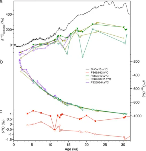
The reconstruction of the history of water mass ventilation relies on the correlation of deep waterΔ¹⁴C‐ values to the atmospheric reference curve (Reimer et al., 2013). The offset between both records will be referred to asΔΔ¹⁴C (‰) hereafter. Throughout the last glacial and into the Holocene, rawΔ¹⁴C‐values of Kerguelen Plateau sediment cores PS69/912 (567 m) and PS69/907‐2 (2,253 m) and Conrad Rise record PS2606‐6 (2,545 m) evolved mostly parallel to each other (Figure 3) Based on this good agreement between the regionally different sediment records, we are confident to use the calibrated data for our reconstructions.

Hereafter, we will report and discuss our results asΔΔ¹⁴C.

At about 30,000 years before present (in the following as ka) records PS69/912 and PS69/907‐2 show similar ΔΔ¹⁴C values of−415‰±76‰and−446‰±53‰ΔΔ¹⁴C. The late glacial and the early Termination (21.6– 17.8 ka) are marked by a rapid decrease in benthicΔΔ¹⁴C of PS69/912 of about 80‰to about −360‰ (Figure 4). Correlating this time period to the atmospheric¹⁴C‐plateau 5 (Sarnthein et al., 2015),−360‰ is the average of three benthicΔ¹⁴C values to the average of atmosphericΔ¹⁴C (Reimer et al., 2013). For more details, please refer to section 2. Both Kerguelen Plateau records as well as Conrad Rise record PS2606‐6 show a second transient decrease in benthicΔΔ¹⁴C during the Antarctic Cold Reversal (ACR) and the Younger Dryas (YD; ~15–12 ka; Figure 4). Between 12 and 5.9 ka, Holocene values of all records lie between

−141‰and−93‰. This period is followed by a constant decrease in deep waterΔΔ¹⁴C down to about

−157‰±10‰(1.8 ka), close to the modern value of Kerguelen Plateau deep water of ~−150‰(Key et al., 2004).

3.2. Stable Carbon Isotopes

Between ~32.8 and 30.5 ka, we record a distinct ~0.5‰increase in PS69/912Δδ¹³C, reaching a maximum value of 2.21‰(Figure 4). Two intervals of increasing planktic‐benthic offsets, parallel to the drops observed in the PS69/912ΔΔ¹⁴C record at 20 and ~13.5 ka (Figure 4), mark theδ¹³C‐evolution throughout the LGM and deglacial. Paralleling the rapidΔΔ¹⁴C increase,Δδ¹³C values reach a minimum of ~0.05‰during the early Holocene (Figure 4). The deglacial trend of decreasingΔδ¹³C shows a brief event of increasing values (~12.03 ka), again paralleled by a similar pattern ofΔΔ¹⁴C (Figure 4). This deglacial decrease is ultimately followed by increasing HoloceneΔδ¹³C values, approaching ~1.14‰(Figure 4f).

4. Modeling

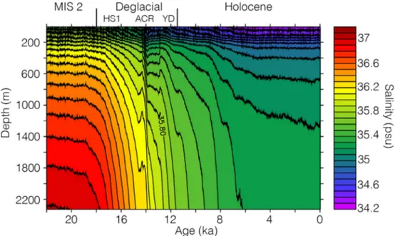
The TraCE‐21ka transient model run (He, 2011; Liu et al., 2009; Liu et al., 2014) indicates pronounced stra- tification and significantly increased salinities for the uppermost 2,300 m in the Indian sector of the Southern Ocean during the LGM (Figure 5). Beginning at about 19 ka, the isohalines start to steepen indi- cating a breakdown of the density stratification. Above ~200 m, however, a strong presence of fresher waters is modeled. Near the end of Heinrich Stadial 1 (HS1) and throughout the ACR, the model simulates a brief return toward more stratified waters, albeit less pronounced than during the glacial. During the YD, isoha- lines and isopycnals steepen again and gradually evolve into the modern water mass geometry throughout the Holocene. During the same time interval, the model also indicates the increasingly pronounced influ- ence of fresher WW above ~400 m. The general pattern of the temporal evolution of stratification is insensi- tive to the exact geographical location in the Indian Ocean AZ (Figure S4).

Several factors affect the temporal changes in the Southern Ocean salinity structure throughout the deglacia- tion, including changes in deep ocean circulation (mainly driven by Northern Hemisphere meltwater hos- ing), surface winds (inducing Ekman transports; see section 4.5), and meltwater input from Antarctica. In particular, the Atlantic Meridional Overturning Circulation slows down during HS1 and starts to recover around 14.7 ka (He, 2011; Liu et al., 2009). An overshoot takes place between 14.5 and 14 ka (ACR) consis- tent with new²³¹Pa/²³⁰Th‐based reconstructions (Mulitza et al., 2017). At nearly the same time, a short but drastic meltwater pulse from Antarctica is introduced in the TraCE‐21ka simulation (He, 2011), which explains the abrupt“jump”in salinity around 14 ka (Figure 5).

5. Discussion

5.1. MIS 3 Ventilation

Compared to the Holocene, the larger radiocarbon depletion during MIS 3 (~30–31 ka), indicates an early reduction in the exchange rate of CDW and surface waters as well as the accumulation of sequestered car- bon in deeper waters (Figure 4). Although atmospheric CO2values of MIS 3 were clearly lower than dur- ing interglacials, the levels were still ~25 ppm higher from ~45 to 31 ka than during the subsequent LGM (Figure 4). We therefore argue that the spatio‐temporal response of the main Southern Ocean sectors to the climatic conditions of MIS 3 was not uniformly pronounced (Adkins, 2013; Kohfeld et al., 2013;

Ronge et al., 2015; Sigman et al., 2010; Sikes et al., 2017; Xiao et al., 2016). While we already record dis- tinctly radiocarbon depleted waters in the Indian Sector, the Pacific (Ronge et al., 2016; Skinner et al., 2015) and the Atlantic Sectors (Skinner et al., 2010) were not yet fully decoupled from the upper ocean, yieldingΔΔ¹⁴C values ~100‰higher than in the Indian Sector. This observation is in good agreement with the deep gateway hypothesis (Sikes et al., 2017) and might indicate the onset of a progressive glacial decoupling of the main Southern Ocean basins. The resulting imbalance might plausibly explain the lower‐than‐interglacial, yet higher‐than‐LGM atmospheric CO2‐values. While the Indian sector of the Southern Ocean was already decoupled from the surface, the Atlantic and Pacific sectors were still venti- lating during MIS3, until the entire deep Southern Ocean was cut‐off from the surface during the LGM (Figure 4).

Figure 3.Kerguelen and Conrad Rise carbon proxy data.(a) AtmosphericΔ¹⁴C (black; SHCal13; Reimer et al., 2013) and marine calibrated paleoΔ¹⁴C; (b) raw Δ¹⁴C data; (c)δ¹³C of PS69/912 (red). Thefilled symbols indicate the planktic data; the empty symbols indicate the benthic data. Due to the high density of samples shown here, the error bars are plotted in Figure 4.

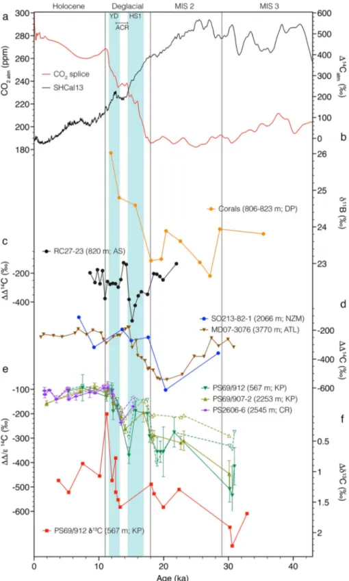
Figure 4.Atmospheric CO₂and Southern Ocean chemistry.(a) Splice of atmospheric CO₂records (red; Köhler et al., 2017) and atmosphericΔ¹⁴C values (black;

SHCal13; Reimer et al., 2013). (b) Deep‐sea coral (dredges; Drake Passage)δ¹¹B‐data (Rae et al., 2018). (c) Intermediate waterΔΔ¹⁴C off Oman (Bryan et al., 2010).

(d) Southern OceanΔΔ¹⁴C (MD07‐3076; Atlantic; Skinner et al., 2010); SO213‐82‐1; Pacific; Ronge et al., 2016). (e) Southern Indian OceanΔΔ¹⁴C (filled symbols) andε¹⁴C (empty symbols; [this study]). (f)Δδ¹³C (red; this study). MIS: Marine Isotope Stage; YD:–Younger Dryas; ACR: Antarctic Cold Reversal; HS1:

Heinrich Stadial 1; DP: Drake Passage; AS: Arabian Sea; NZM: New Zealand Margin; ATL: South Atlantic; KP: Kerguelen Plateau; CR: Conrad Rise. The blue bars mark the YD and HS1.

5.2. Impact of Hydrothermal Vent Systems

Ronge et al. (2016) hypothesized an impact of hydrothermal CO2 —barren of ¹⁴C— on foraminiferal radiocarbon values and inferred ventilation ages. In the following years, other paleoceanographic studies could identify and verify this mechanism as an influence on marine¹⁴C‐values (e.g., Stott et al., 2019).

Lacking any radiocarbon, mantle‐derived CO2, would indicate sample ages exceeding the¹⁴C‐timescale.

Hence, hydrothermal CO2has the potential of increasing deep water ventilation ages, resulting in very lowΔΔ¹⁴C records. Several active spreading centers and hydrothermal vent systems are known for the southern Indian Ocean (Ardyna et al., 2019; Tao et al., 2012). Using WOCEδ³He‐data (Talley, 2013), we traced a hydrothermal plume, emanating from the Southwest Indian Ridge (SWIR), downstream into the direction of our research area (Figure 6). Most pronounced between 60°S and 50°S, and 20°E and 40°

E, the plume moves along the ACC between ~500 m and 2,000 m water depth (Figure 6). Toward the Kerguelen Plateau, the depth of the plume gradually deepens, to approximately 1,500 m west of it. As shown in Figure 6, both records—PS69/907‐2 and PS69/912—are located in waters not directly affected by the modern plume. However, given the fact of increased glacial hydrothermal and mid‐ocean ridge (MOR) activity (Hasenclever et al., 2017; Lund et al., 2016; Stott & Timmermann, 2011; Tolstoy, 2015) and increased stratification of the Indian sector of the Southern Ocean (paragraphs 3.4/4.4), it is likely that the hydrothermal activity of the SWIR and other systems exposed a larger region to low¹⁴C waters.

Hence, a breakdown of stratification would result in the upwelling of ¹⁴C‐depleted waters and might result in the two phases of decreasing ΔΔ¹⁴C in PS69/912 and to some extent in PS69/907‐2 (Figure 4). CO2 released at volcanic arc systems yields δ¹³C‐values very similar to that of sedimentary carbonates (Lupton et al., 2006; Stott & Timmermann, 2011) as the subducted carbon from marine sedi- ments is directly transformed into CO2(Coltice et al., 2004). Hence, arc‐derived CO2would have no sig- nificant impact on water mass δ¹³C values. MORs on the other hand are directly fed by the upper mantle, whereδ¹³C is close to−5‰(Coltice et al., 2004). The release of CO2along MOR can thus drive water massδ¹³C toward more negative values. Similar toΔΔ¹⁴C, increased glacial SWIR volcanism in combination with a more stratified water column has the potential to significantly influence southern Indian Ocean δ¹³C‐values. However, in accordance with Ronge et al. (2016), we propose that without the changes in oceanic circulation and ventilation discussed in this paper, SWIR volcanism alone seems unlikely to account for the¹⁴C and¹³C changes observed by us.

Figure 5.Temporal evolution of the vertical salinity structure in the Indian Ocean sector of the Southern Ocean (averaged over the area 40°E–110°E and 45°S–65°

S) as simulated by TraCE‐21ka. HS1: Heinrich Stadial 1; ACR: Antarctic Cold Reversal; YD: Younger Dryas.

5.3. Impact of Clathrates

Similar to MOR‐derived CO2, the decay of clathrates can also significantly affect marine carbon isotopes.

While CO2clathrates are only depleted in¹⁴C (Stott & Timmermann, 2011), methane clathrates are also extremely depleted inδ¹³C (Maslin et al., 2010). The stability zone of these clathrates lies at a water depth of approximately 400 m (Stott & Timmermann, 2011). Given the reduced glacial sea level, decaying clath- rates under warming conditions could thus have contributed to theΔΔ¹⁴C/δ¹³C signal observed in the shal- low record of PS69/912 (567 m). Both other cores, PS69/907‐2 (2253 m) and PS2606‐6 (2545 m), however, are located well below the 400‐m threshold for clathrates stability. As theΔΔ¹⁴C‐pattern of both deeper cores parallels to some extent the shallow PS69/912 signal, but cannot be explained by clathrate‐(in)stability, we argue that this process is an unlikely driver for the patterns observed in these three records.

5.4. Impact of Salinity Stratification

Although the shallow core PS69/912 is today bathed by upwelling UCDW (Figure 2; Garcia et al., 2014;

Locarnini et al., 2013; Park et al., 2008; van Beek et al., 2008), it is noteworthy that throughout the entire interval covered in this study, this water depth was bathed by waters similarly radiocarbon depleted as LCDW, as reflected by core PS69/907‐2 (modern LCDW; Figure 2). In the AZ, located between Antarctica and the APF, cold subsurface WW is found beneath a warmer and fresher layer of surface water (Park et al., 1998). A pronounced halocline, thermocline, and pycnocline mark the boundary from WW to the sur- face mixed layer, while the lower boundary to the UCDW is also marked by a strong (but less pronounced) vertical gradient (Park et al., 1998). In combination with an increase in the extent of Antarctic sea ice (Xiao et al., 2016), the vertical salinity gradient in our research area might have been even more pronounced dur- ing the last glacial (Figure 5). As the degree of nutrient consumption, or the efficiency of the biological Figure 6.Hydrothermalδ³He concentrations (Talley, 2013). Sections as indicated in Figure 1.(a) North‐south section (II in Figure 1). (b) West‐east section (III in Figure 1). PS69 sediment cores (colored dots) were projected into the section (B) to indicate their depth relation to theδ³He plume.

carbon pump, is positively linked to the amount of CO2entering or escaping the ocean, a strengthened halo- cline ultimately affects atmospheric CO2levels (Haug et al., 1999) by cutting off surface waters from upwel- ling nutrients. Using the CCSM3 model, Ronge et al. (2015) showed a pronounced surface input of freshwater due to melting sea ice in close proximity to the formation region of Antarctic Intermediate Water (AAIW). Compared to preindustrial values, the salinity of glacial Southwest Pacific surface and inter- mediate waters dropped by up to 1.5‰(Ronge et al., 2015). This decrease in combination with the elevated deep water salinity observed by Adkins (2013) significantly increased the salinity gradient and thus the stra- tification of the glacial water column. In the Indian sector of the Southern Ocean, however, the TraCE‐21ka simulation indicates that the presumed glacial salinity anomaly was even more pronounced than in the southwest Pacific (Figure 5). We assume that the increased salinity strengthened the glacial halocline of the southern Indian Ocean by an intensification of the salinity gradient of the entire water column, with fresher waters above ~400 m—in particular above 200 m—and higher salinities below. This increase in the salinity gradients and the resulting stratification is clearly displayed by the transient TraCE‐21ka model run between ~22 and ~19 ka (Figure 5).

5.5. Glacial to Deglacial Dynamics

The combined effects of the more pronounced glacial stratification and weakened upwelling ultimately resulted in the observed decoupling of shallow (PS69/912) to middepth waters (records below ~2,500 m) from surface waters. Along with the glacial expansion of Antarctic sea ice (Xiao et al., 2016) and a potential displacement of wind systems (Menviel et al., 2018; Van der Putten et al., 2015), these factors likely contrib- uted to the accumulation of old, sequestered biogenic carbon, and perhaps to some extent MOR‐derived vol- canic CO2in glacial deep waters of the lower cell (Figure 4).

Despite being close to the potential upwelling area of old, sequestered carbon, studies from the glacial and deglacial New Zealand Margin (Ronge et al., 2016; Rose et al., 2010) noted no or no significant depletion of intermediate waterΔΔ¹⁴C above ~2,000 m water depth, throughout this time period. However, the recon- structedΔ¹⁴C of sediment record PS69/912 (567 m) indicates the presence of a water mass low in¹⁴C and δ¹³C with an offset most pronounced to atmospheric values during MIS 3 and the LGM (Figure 4).

Beginning at about 30 ka, ΔΔ¹⁴C and Δδ¹³C values start to increase/decrease toward the Holocene (Figure 4). The apparent incongruity between the shallow Pacific and our new Indian Ocean sites might be explained by the different water masses these cores record. The more northerly Pacific sites (De Pol‐Holz et al., 2010; Ronge et al., 2016; Rose et al., 2010) are bathed by“recently”formed AAIW. As described above, PS69/912 on the other hand directly records the upwelling branch of“older” UCDW (Figure 2). Coral dredges that were performed at a similar latitude in the Drake Passage and off Tasmania also recorded upwelling CDW (Burke & Robinson, 2012; Hines et al., 2019). Converted to epsilonε¹⁴C data (as used by Hines et al., 2019), Drake Passage data show similar values as recorded by PS69/907‐2, while the Tasman Sea corals that are located further to the north than the Drake Passage and our Kerguelen records show higher glacial values and might be indicative of a reduce influence of Pacific Deep Water (Figure S5;

Burke & Robinson, 2012; Hines et al., 2019). At the end of the LGM, however,ΔΔ¹⁴C at 567 m (PS69/912) decreased by ~80‰, Δδ¹³C increased by ~0.3‰, and showed a decoupled trend from the atmosphere.

TheseΔΔ¹⁴C‐values are about 110‰lower than values from the intermediate Southwest Pacific (Ronge et al., 2016; Rose et al., 2010). The transientΔΔ¹⁴C/Δδ¹³C‐signal between ~21 and ~17.5 ka coincided with the pattern of deep water rejuvenation observed in the downstream southwest Pacific (Ronge et al., 2016) and upstream South Atlantic (Skinner et al., 2010). Some authors, however, suggested that the observed decline in global oceanicΔ¹⁴C mirrors the atmospheric pattern and is rather a sign of a decreased global

14C inventory, instead of a redistribution and aging of different carbon inventories (Zhao et al., 2018). It was shown that many deep water records parallel atmosphericΔ¹⁴C, with a somewhat higher deep water‐ to‐atmosphere offset during the glacial compared to the deglacial and Holocene (Zhao et al., 2018). To some extent, our reconstructions are consistent with these results, also showing a roughly parallel evolution of Indian Ocean deep water and atmospheric values, indicating a longer timescale increase inΔΔ¹⁴C and deep waterδ¹³C (Figure 3; Reimer et al., 2013). However, both transient phases of droppingΔΔ¹⁴C‐values (~21–17 ka; ~15–12 ka) occur independent from the atmosphere, are similarly pronounced when converted toε¹⁴C, and indicate the presence of a¹⁴C‐depleted water mass. This conclusion is also supported by ourδ¹³C recon- structions that parallel the¹⁴C‐pattern, also arguing for old‐sequestered carbon, maybe amplified to some

extent by the additional injection of hydrothermal CO2. Therefore, we argue that upwelling of radiocarbon depleted, lowδ¹³C deep waters is a likely driver of upper South Indian Ocean¹⁴C and¹³C during the degla- cial transition. This interpretation is in line withδ¹¹B reconstructions from coral dredges in the Drake Passage (Rae et al., 2018) that highlight a drop in UCDW pH, interrupting the long‐term pH increase—indi- cative for a simultaneous injection of old and CO2‐rich waters—during the same time interval (Figure 4).

Steepening pycnoclines also indicate the onset of stratification breakdown in the transient model simulation (Figure 5). Intermediate‐water records from the Arabian Sea off Oman (RC27‐14 596 m; RC27‐23 820 m) as well seem to show the incorporation of old and radiocarbon depleted waters throughout the last deglacial period (Figure 4; Bryan et al., 2010). Despite lacking conclusive evidence from Southern Ocean intermediate‐water records (De Pol‐Holz et al., 2010; Rose et al., 2010; Siani et al., 2013), it was suggested that the Arabian Sea signal implies the upwelling of¹⁴C‐depleted waters in the Southern Ocean and their transport to the lower latitudes via Antarctic Intermediate or Subantarctic Mode Waters (Bryan et al., 2010). However, as both RC27 sediment cores (Bryan et al., 2010) are located within the modern stability zone of CO2‐clathrates (Stott & Timmermann, 2011; paragraph 4.3) deglacial warming might also have trig- gered the decomposition of clathrates in intermediate waters off Oman. This process could also release¹⁴C‐ depleted CO2into the water column, thus explaining the deglacialΔΔ¹⁴C‐excursions observed by Bryan et al. (2010). Furthermore, the waters off Oman are located in a modern upwelling area (Anderson &

Lucas, 2008). Thus, old deep waters might have come into direct contact with overlying intermediate waters, bypassing the loop via the Southern Ocean. Given that other Southern Ocean intermediate water records clo- ser to the formation of AAIW did not see the incorporation of¹⁴C depleted waters during the deglacial (De Pol‐Holz et al., 2010; Ronge et al., 2016; Rose et al., 2010), it is difficult to assess, whether or not the Oman records (Bryan et al., 2010) really show the incorporation of¹⁴C depleted AAIW. A reevaluation of surface reservoir ages used to assess Southeast Pacific AAIW ventilation, however (De Pol‐Holz et al., 2010), shed new light on the transport of upwelled ¹⁴C‐depleted water to this location, via the CDW‐AAIW loop (Siani et al., 2013). Thus, we propose a similar mechanism as a likely process for the Oman signal via the Indian part of the deep carbon pool, located in the returnflow of glacial IDW. As one of the first true Southern Ocean shallow‐water records, PS69/912 shows a significant drop in deglacialΔΔ¹⁴C. The transfer of old,¹⁴C‐depleted carbon from the mid‐depth carbon pool (Cook & Keigwin, 2015; Ronge et al., 2016;

Skinner et al., 2010; Umling & Thunell, 2017) to the surface likely caused this decrease. In the AZ, a part of the oceanic,¹⁴C‐depleted, lowδ¹³C CO2was released to the atmosphere, contributing to patterns of atmo- spheric CO2(Köhler et al., 2017),δ¹³C (Schmitt et al., 2012) andΔ¹⁴C (Reimer et al., 2013). Due to incom- plete nutrient consumption and the short residence time at the surface however (Watson et al., 2015), a significant amount of¹⁴C‐depleted waters was possibly fed into subducting AAIW, transported to the north, before it fully equilibrated with the atmosphere. Both the HS1 and the YD decline in intermediate water ΔΔ¹⁴C off Oman (Bryan et al., 2010) were preceded by increasing SOΔΔ¹⁴C as observed in PS69/912 and to some extent in PS69/907‐2 and PS2606‐6 (Figure 4). During both time intervals, the modeled isohalines strongly steepened (Figure 5) associated with a pronounced destratification, which opened a pathway for

14C‐depleted, lowδ¹³C, CO2‐rich deep waters to the surface. Based on Antarctic ice core records, it has recently been shown that North Atlantic cold events induced poleward strengthening of the southern wes- terly winds, which is simulated by CCSM3 TraCE‐21ka (Buitzert et al., 2018). Through enhanced Ekman transport and surface divergence, the shift in the westerlies amplified upwelling of deep waters to the sur- face. At the depth of PS69/907‐2 (2,253 m), the TraCE‐21ka model experiment highlights two intervals of decreasing salinity gradients at the time of both pulses observed in PS69/912‐3 ΔΔ¹⁴C (Figure S6).

Although PS69/907‐2 is not directly upstream of shallow record PS69/912, its data and the modeling results indicate that upwelling of radiocarbon‐depleted waters from the middepth Southern Ocean might have influenced the shallow site and also surface waters. Ultimately, the rejuvenation of circumpolar deep waters might have closed the loop from the deep Indian Ocean, via the Southern Ocean (this study) to the low ΔΔ¹⁴C values, observed in intermediate waters off Oman during the deglaciation (Bryan et al., 2010).

5.6. Indian Ocean Ventilation During the YD

The transient drop inΔΔ¹⁴C in all three sediment cores (~15–12 ka) and the subsequent rise (Figure 4e) marks a fundamental difference to other radiocarbon records from the Southern Ocean (e.g., Chen et al., 2015; Ronge et al., 2016; Rose et al., 2010; Skinner et al., 2010; Skinner et al., 2015). In the South Atlantic

and South Pacific, ventilation reached Holocene‐like values at the end of HS1 and did not significantly con- tribute to the pattern of atmospheric CO2thereafter (Figure 4d). At the end of the YD,δ¹³C values of benthic and planktic foraminifers converge and indicate an active ventilation and a pronounced equilibration of CDW and surface waters of the Southern Indian Ocean (Figure 4f). So far, the release of CO₂from thawing permafrost soils (Köhler et al., 2014; Winterfeld et al., 2018) or the decrease in biological primary production (Hertzberg et al., 2016) were considered as the main drivers of the second increase in atmospheric CO2dur- ing the YD. With our new data from both Kerguelen records (PS69/912 and PS69/907‐2) and also the Conrad Rise (PS2606‐6), we are for thefirst time able to show that the Southern Ocean likely contributed to the YD increase in atmospheric CO2(Figure 4). During this time period, the Indian sector of the Southern Ocean actively ventilated ¹⁴C‐ and ¹³C‐depleted deep waters. However, after the transformation of CDW to AAIW, ¹⁴C‐depleted waters that were not completely equilibrated with the atmosphere were possibly exported toward the north and decreased the radiocarbon content of intermediate waters in the Arabian Sea (Bryan et al., 2010). The comparison of our Southern Ocean records and the Drake Passage and Tasman coral records (Figure S5; Burke & Robinson, 2012; Hines et al., 2019) further highlights the impor- tance of the Indian sector and its role in the deglacial carbon cycle. Both records reach modern‐likeε¹⁴C values before the onset of the YD and do not show any excursion during the second rise in atmospheric CO2(Figure S5).

Following the deglacial breakdown in stratification, all records from the Kerguelen Plateau and the Conrad Rise show similarΔ¹⁴C‐values during the late YD, throughout the Holocene and progressively evolve paral- lel to the atmospheric pattern (Figure 4).

6. Conclusions

Our combination of new radiocarbon andδ¹³C data from the Kerguelen Plateau and the Conrad Rise with state‐of‐the‐art climate modeling allowed us to assess the contribution of the southern Indian Ocean in the glacial‐deglacial carbon cycle. Our reconstructions and simulations show that the deep Indian Ocean was an integral part of the glacial ocean carbon pool and that it acted as a conduit for old, radiocarbon‐depleted, and CO2‐rich deep waters to the surface and into intermediate waters. In detail, we conclude the following:

1. Below a pronounced cap of fresher waters, glacial water masses (200–2,300 m) were marked by a pro- nounced stratification and significantly increased salinities. Both the layer of fresher waters and the stra- tified more saline waters allowed for the glacial accumulation of radiocarbon depleted CDW up to a depth as shallow as 567 m (PS69/912) and even shallower when the low LGM sea level is taken into account.

2. At ~19 ka, the isohalines began to steepen and triggered a breakdown of the prevailing stratification. The decreased stratification allowed for the ventilation of Circumpolar Deep Waters, the release of CO₂to the atmosphere, and the subsequent incorporation of¹⁴C‐depleted waters in intermediate waters that were observed in the Arabian Sea.

3. Toward the end of HS1 and into the ACR, the isopycnalsflattened again, marking a brief return toward a more stratified water column. The increase in stratification triggered decreasing water mass radiocarbon values at the Kerguelen Plateau and the Conrad Rise (Figures 4 and 5).

4. During the YD, isopycnals steepen, once again eroding the stratification. This process triggered a second pulse of CDW ventilation. At all sitesΔΔ¹⁴C andΔδ¹³C proxies point toward increasing ventilation dur- ing the YD (Figure 4). This increase coincided with the YD rise in atmospheric CO₂and decreasing down- stream radiocarbon values in the Arabian Sea.

5. In contrast to the Atlantic and Pacific sectors of the Southern Ocean, the Indian Ocean most likely con- tributed to the second deglacial rise in atmospheric CO₂.

6. A circumpolar picture of upwelling, ventilation, and circulation processes is necessary to fully under- stand the transition from the last glacial to the current interglacial.

References

Adkins, J. F. (2013). The role of deep ocean circulation in setting glacial climates.Paleoceanography,28, 539–561.

Adkins, J. F., & Boyle, E. A. (1997). Changing atmosphericΔ¹⁴C and the record of deepwater paleoventilation ages.Paleoceanography, 12(3), 337–344.

Acknowledgments

We would like to thank captains and crews of R/V Polarstern expeditions PS30 and PS69, E. Bonk, B. Diekmann, J. Gottschalk, H. Grotheer, R.

Fröhlking‐Teichert, J. Hollop, S.

Jaccard, A. Mackensen, M. Sarnthein, V. Schumacher, L. Schönborn, M.

Seebeck, and S. Wiebe for technical support, data, and discussions. Thanks to P. Rafter for the creation of the awesome, Wes Anderson themed ODV color scheme. T. A. R. was funded by theDeutsche Forschungs Gemeinschaft (DFG) Antarctic Priority Program SPP1158, project RO5057/1‐2, and the joint MARUM/AWI project POSY. We would also like to acknowledge AWI project COPTER for helpful discussions and input. We thank F. He, Z. Liu, and B. Otto‐Bliesner for making available the TraCE‐21ka model output via the Earth System Grid (NCAR). M. P.

acknowledges support from the Bundesministerium für Bildung und Forschung (BMBF) through the PalMod initiative. We thank Editor E.

Thomas, Associate Editor H. Bostock, and two reviewers for their helpful comments. Data available at https://

doi.pangaea.de/10.1594/

PANGAEA.906365.

Anderson, T. E., & Lucas, M. I. (2008). Upwelling ecosystems. In S. E. Jorgensen, & B. Fath (Eds.),Encyclopedia of Ecology, (pp. 3651–3661).

New York: Elsevier Science.

Ansorge, I. J., Roman, R., Durgadoo, J. V., Ryan, P. G., Diamini, L., Gebhardt, Z., et al. (2008). Thefirst oceanographic survey of the Conrad Rise.South African Journal of Science,104, 333–336.

Ardyna, M., Lacour, L., Sergi, S., d'Ovidio, F., Sallée, J.‐B., Rembauville, M., et al. (2019). Hydrothermal vents trigger massive phyto- plankton blooms in the Southern Ocean.Nature Communications,10, 2451.

Broecker, W. (2009). The mysterious¹⁴C decline.Radiocarbon,51(1), 109–119.

Broecker, W., & Barker, S. (2007). A 190‰drop in atmosphere'sΔ¹⁴C during the“Mystery Interval”(17.5 to 14.5 kyr).Earth and Planetary Science Letters,256, 90–99.

Broecker, W., Barker, S., Clark, E., Hajdas, I., Bonani, G., & Stott, L. (2004). Ventilation of the glacial deep Pacific Ocean.Science,306, 1169–1172.

Broecker, W., & Clark, E. (2010). Search for a glacial‐age¹⁴C‐depleted ocean reservoir.Geophysical Research Letters,37, L13606.

Broecker, W., Clark, E., & Barker, S. (2008). Near constancy of the Pacific Ocean surface to mid‐depth radiocarbon‐age difference over the last 20 kyr.Earth and Planetary Science Letters,274, 322–326.

Bryan, S. P., Marchitto, T. M., & Lehman, S. J. (2010). The release of¹⁴C‐depleted carbon from the deep ocean during the last deglaciation:

Evidence from the Arabian Sea.Earth and Planetary Science Letters,298, 244–254.

Buizert, C., Sigi, M., Severi, M., Markle, B., Wettstein, J. J., McConnell, J. R., et al. (2018). Abrupt ice‐age shits in southern westerly winds and Antarctic climate forced from the north.Nature,563(7733), 681–685. https://doi.org/10.1038/s41586‐018‐0727‐5

Burke, A., & Robinson, L. F. (2012). The Southern Ocean's role in carbon exchange during the last deglaciation.Science,335(6068), 557–561. https://doi.org/10.1126/science.1208163

Burke, A., Stewart, A. L., Adkins, J. F., Ferrari, R., Jansen, M. F., & Thompson, A. F. (2015). The glacial mid‐depth radiocarbon bulge and its implications for the overturning circulation.Paleoceanography,30, 1021–1039.

Butzin, M., Köhler, P., & Lohmann, G. (2017). Marine radiocarbon reservoir age simulations for the past 50,000 years.Geophysical Research Letters,44(16), 8473–8480.

Butzin, M., Prange, M., & Lohmann, G. (2012). Readjustment of glacial radiocarbon chronologies by self‐consistent three‐dimensional ocean circulation modeling.Earth and Planetary Science Letters,317‐318, 177–184.

Chen, T., Robinson, L. F., Burke, A., Southon, J. R., Spooner, P., Morris, P. J., & Ng, H. C. (2015). Synchronous centennial abrupt events in the ocean and atmosphere during the last deglaciation.Science,349(6255), 1537–1541. https://doi.org/10.1126/science.

aac6159

Collins, W. D., Bitz, C. M., Blackmon, M. L., Bonan, G. B., Bretherton, C. S., Henderson, T. B., et al. (2006). The Community Climate System Model Version 3 (CCSM3).Journal of Climate,19, 2122–2143.

Coltice, N., Simon, L., & Lécuyer, C. (2004). Carbon isotope cycle and mantle structure.Geophysical Research Letters,31, L05603.

Cook, M. S., & Keigwin, L. D. (2015). Radiocarbon profiles of the NW Pacific from the LGM and deglaciation: Evaluating ventilation metrics and the effect of uncertain surface reservoir ages.Paleoceanography.

De Pol‐Holz, R., Keigwin, L. D., Southon, J., Hebbeln, D., & Mohtadi, M. (2010). No signature of abyssal carbon in intermediate waters off Chile during deglaciation.Nature Geoscience,3, 192–195.

DeVries, T., & Primeau, F. (2010). An improved method for estimating water‐mass ventilation age from radiocarbon data.Earth and Planetary Science Letters,295, 367–378.

Dezileau, L., Bareille, G., Reyss, J.‐L., & Lemoine, F. (2000). Evidence for strong sediment redistribution by bottom currents along the southeast Indian ridge.Deep Sea Research, Part I,47, 1899–1936.

Durgadoo, J. V., Lutjeharms, J. R. E., Biastoch, A., & Ansorge, I. J. (2008). The Conrad Rise as an obstruction to the Antarctic Circumpolar Current.Geophysical Research Letters,35, 1–6.

Garcia, H. E., Locarnini, R. A., Boyer, T. P., Antonov, J. I., Baranova, O. K., Zweng, M. M., et al. (2014). World Ocean Atlas 2013, Volume 3:

Dissolved oxygen, apparent oxygen utilization, and oxygen saturation. In S. Levitus & A. V. Mishonov (Eds.),World Ocean Atlas 13:

NOAA.

Gottschalk, J., Szidat, S., Michel, E., Mazaud, A., Salazar, G., Battaglia, M., et al. (2018). Radiocarbon measurements of small‐size fora- miniferal samples with the Mini Carbon Dating System (MICADAS) at the University of Bern: Implications for paleoclimate recon- structions.Radiocarbon,60, 469–491.

Hasenclever, J., Knorr, G., Rüpke, L. H., Köhler, P., Morgan, J., Garofalo, K., et al. (2017). Sea level fall during glaciation stabilized atmospheric CO2by enhanced volcanic degassing.Nature Communications,8, 15867.

Haug, G. H., Sigman, D. M., Tiedemann, R., Pedersen, T. F., & Sarnthein, M. (1999). Onset of permanent stratification in the subarctic Pacific Ocean.Nature,401, 779–782.

He, F. (2011). Simulating Transient Climate Evolution of the Last Deglaciation With CCSM3, Ph.D. Thesis.

Hertzberg, J. E., Lund, D. C., Schmittner, A., & Skrivanek, A. L. (2016). Evidence for a biological pump driver of atmospheric CO2rise during Heinrich Stadial 1.Geophysical Research Letters,43, 12,242–212,251.

Hines, S. K. V., Eiler, J. M., Southon, J. R., & Adkins, J. F. (2019). Dynamic intermediate waters across the late glacial revealed by paired radiocarbon and clumped isotope temperature records.Paleoceanography and Paleoclimatology,34, 1074–1091.

Jacot Des Combes, H., Esper, O., De La Rocha, C. L., Abelmann, A., Gersonde, R., Yam, R., & Shemesh, A. (2008). Diatomδ¹³C,δ¹⁵N, and C/N since the Last Glacial Maximum in the Southern Ocean: Potential impact of species composition.Paleoceanography,23(4), 2008PA001589.

Johnson, K. (2007). Kerguelen Plateau benthic foraminifera as a proxy for Late Neogene water mass history and Antarctic glacial‐deglacial cycles. Paper presented at the 10th ISAES X.

Katsuki, K., Ikehara, M., Yokoyama, Y., Yamane, M., & Khim, B.‐K. (2012). Holocene migration of oceanic front systems over the Conrad Rise in the Indian Sector of the Southern Ocean.Journal of Quaternary Science,27(2), 203–210.

Key, R. M., Kozyr, A., Sabine, C. L., Lee, K., Wanninkhof, R., Bullister, J. L., et al. (2004). A global ocean carbon climatology: Results from Global Data Analysis Project (GLODAP).Global Biochemical Chycles,18, 1–23.

Kohfeld, K. E., Graham, R. M., de Boer, A. M., Sime, L. C., Wolff, E. W., Le Quéré, C., & Bopp, L. (2013). Southern Hemisphere westerly wind changes during the Last Glacial Maximum: paleo‐data synthesis.Quaternary Science Reviews,68, 76–95.

Köhler, P., Knorr, G., & Bard, E. (2014). Permafrost thawing as a possible source of abrupt carbon release at the onset of the Bølling/Allerød.

Nature Communications,5, 5520.

Köhler, P., Nehrbass‐Ahles, C., Schmitt, J., Stocker, T. F., & Fischer, H. (2017). A 156 kyr smoothed history of the atmospheric greenhouse gases CO2, CH4, and N2O and their radiative forcing.Earth System Science Data,9, 363–387.