JHEP01(2015)139
Published for SISSA by Springer Received: November 17, 2014 Accepted: January 9, 2015 Published: January 27, 2015
The renormalon diagram in gauge theories on R
3× S
1Mohamed M. Anbera,b and Tin Sulejmanpasicc,d
aInstitut de Th´eorie des Ph´enom`enes Physiques, ´Ecole Polytechnique F´ed´erale de Lausanne, CH-1015 Lausanne, Switzerland
bDepartment of Physics, University of Toronto, Toronto, ON M5S 1A7, Canada
cDepartment of Physics, North Carolina State University, Raleigh, NC, 27695, U.S.A.
dInstitute for Theoretical Physics, University of Regensburg, 93040 Regensburg, Germany
E-mail: mohamed.anber@epfl.ch,
tin.sulejmanpasic@physik.uni-regensburg.de
Abstract: We analyze the renormalon diagram of gauge theories on R3 ×S1. In par- ticular, we perform exact one loop calculations for the vacuum polarization in QCD with adjoint matter and observe that all infrared logarithms, as functions of the external mo- mentum, cancel between the vacuum part and finite volume part, which eliminates the IR renormalon problem. We argue that the singularities in the Borel plane, arising from the topological neutral bions, are not associated with the renormalon diagram, but with the proliferation of the Feynman diagrams. As a byproduct, we obtain, for the first time, an exact one-loop result of the vacuum polarization which can be adapted to the case of thermal compactification of QCD.
Keywords: Solitons Monopoles and Instantons, Nonperturbative Effects, Renormaliza- tion Regularization and Renormalons
ArXiv ePrint: 1410.0121
JHEP01(2015)139
Contents
1 Introduction 1
2 IR renormalons: the sickness and cure 5
2.1 IR renormalons onR4 5
2.2 Overview of the theory onR3×S1 and the absence of the renormalon problem 7
3 Strategy and the calculation method 9
3.1 Perturbative dynamics of QCD(adj) on R3×S1 10
3.2 The background field method onR3×S1in the presence of non-trivial holonomy 11
3.3 The general form of the gluon propagator 14
4 Calculating the polarization tensor onR3×S1 15
4.1 The one-loop fermion correction 15
4.2 The non-abelian part of QCD one-loop correction 17
5 The static limit, resummation and absence of IR renormalons 18
6 Conclusion 20
A Lie algebra and propagators on R3 ×S1 in the presence of holonomy 22
A.1 Elements of the Lie algebra 22
A.2 The propagator in the presence of background holonomy 22
B The Matsubara sums 24
C Integrals 26
D The results of the integrals 26
E The computations of integrals 27
1 Introduction
Non-abelian gauge theories on R3 ×S1 with center symmetry have been of great inter- est [1–7] in the past years, not only as a tool for understanding QCD-like theories in a controlled, semi-classical regime, but potentially as a way to define a theory on R4 by arguing continuity in the compact circumference L of the circle [8, 9]. There has been tremendous progress in understanding the dynamics of the theory forLΛQCD−1, which is carried either by instanton-monopoles or bound states of instanton-monopoles known asbions.
JHEP01(2015)139
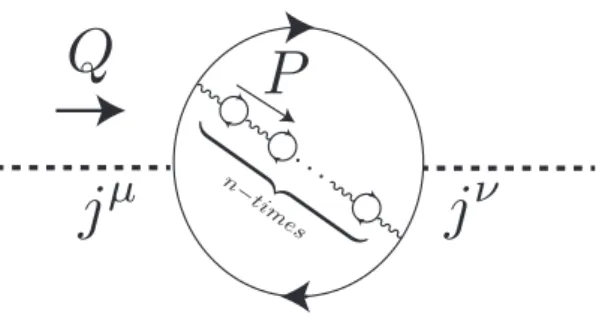
Figure 1. Typical renormalon diagram.
On the other hand, non-abelian gauge theories on R4 are strongly coupled, and non- perturbative effects are notable. Even so, one may still hope that certain processes at short distance scales, or large momentum transfer1 Q2Λ2QCD, are computable in perturbation theory. In a certain class of n loop diagrams, however, the characteristic momentum running through the loops is not Q2, but is exponentially suppressed with the number of loopsn. This suppression is caused by the appearance of logarithms in the one loop vacuum polarization diagrams (see section2and [10,11] for more details.), which we revisit in this work onR3×S1. This suppression leads ton! growth of the diagram upon integration over the momentumP running through the chain of loops (see figure1 for a typical diagram), rendering the loop expansion non-Borel summable (for review see [10,11]). Another way of saying this is that the Borel plane contains poles on the real axis, which generate ambiguities in the calculation, depending on whether the pole is circumvented from above or from below.
The class of diagrams suffering from this problem are referred to asthe renormalon diagrams and the corresponding non-Borel summability is the (in)famousrenormalon problem [12].
Borel non-summability of the perturbation theory is not in itself surprising and was argued by Dyson long time ago2[14]. This problem also appears in quantum mechanics, but there the divergence is caused by the factorial proliferation of the number of the Feynman diagrams. In fact, one finds that such divergence is cured by instanton-anti-instanton events [15,16], and a priori has nothing to do with the renormalon problem.
It was recently suggested in [17,18] that IR renormalon ambiguity cancellation can be understood in terms of semi-classical instanton-monopole solutions appearing in the theory on R3×S1, but which do not appear on R4. This idea was substantiated by the detailed analysis of two-dimensional models onR×S1 [19–22], which have extra non-perturbative saddles compared to the theory onR2 (these are analogous to the instanton-monopoles in gauge theories). Since these theories reduce to quantum mechanics for smallL, a resurgent expansion can be constructed, in which case these saddles play a crucial role in canceling the ambiguities of the perturbation theory. It was conjectured in these works that these saddles (or rather their correlated pairs) cancel the renormalon ambiguity which also exists
1Capital letters are used to denote the 4-momenta, and small letters denote the spatial 3-momenta.
2Although it is true that the perturbation series is divergent, it was pointed out that Dyson’s argument may not be entirely valid [13].
JHEP01(2015)139
in these theories onR2. This conjecture was made plausible because the leading renormalon ambiguity matched the even-integer multiple of the action of the saddles, because the beta- function coefficient, β0, is an integer. This, however, is not the case in gauge theories in four dimensions where the beta-function coefficient β0 is no longer an integer. This non- matching in gauge theories has led to the conjecture that renormalon ambiguities are shifted on R3×S1 and that they smoothly interpolate from a semi-classical regime atLΛ−1QCD to those in the decompactification limitL→ ∞ [18].
In this work, however, we show that the renormalon problem3vanishes completely from theories formulated onR3×S1. In particular, we will show that all logarithmic dependence of the vacuum polarization (which we calculate exactly for arbitrary external momentum) in a center symmetric background cancel out, and hence no renormalon problem appears in the theory. In order to preserve the center symmetry, we will mainly focus on Yang-Mills theory with adjoint matter, where center symmetry is perturbatively stable [1].
For the theory on a small4 L Λ−1QCD, the IR dynamics of QCD(adj) is governed by the instanton-monopoles and their correlated pairs which are called bions. The neutral monopole-anti-monopole pairs (the neutral bions) generate ambiguities which should be canceled by the perturbation theory and which were conjectured to be the semi-classical re- alization of renormalons [17–19,21]. Since we show that no renormalons exist in this theory, the inevitable conclusion is that the singularity in the Borel plane due to neutral bions is as- sociated with the proliferation of diagrams, rather than the renormalon.5 On the other hand the factorial divergence of diagrams onR4 is believed to be associated to the 4D instanton- anti-instanton pairs. This is consistent with the fact that no factorial growth of diagrams happens in the largeN limit [23], as instantons have an exponentially vanishing contribu- tion in this limit. The arguments leading to this conclusion should fail however onR3×S1, provided that the largeN limit is taken withN Lkept fixed,6as the ambiguities of the neu- tral bions (which survive this kind of largeN limit) need to be canceled by an appropriate n! growth. Since no renormalons exist onR3×S1 it is natural to assume that this factorial behavior will come from some additional diagrams which appear in the theory on R3×S1. Although the perturbation theory does not suffer from the IR renormalons, this should by no means be taken as an indication that the perturbation theory is complete. One imme- diate indication of this is that computation of the renormalon processes are very sensitive to the radiusL, which they should not be since the full theory is gapped and should not feel
3We emphasize that in this paper we define renormalons as the ambiguities in the Borel plane which arise from the factorial growth of the diagram shown in figure1. We stress, however, that the word renormalon can also be used in a broader sense to mean any high-order growth of perturbation theory which can not be accounted for by instantons. In addition the word renormalon is often used in the context of OPE matching (see discussion at the end of section2.1).
4Strictly speaking the criterion should beN L Λ−1QCD, but since we mostly discuss N = 2,3 in this work, this difference is not important.
5Although the authors of [19,21,22] do not stress this point, the cancellation between non-perturbative saddles and perturbation theory is clearly of this kind.
6Since the relevant scale in the center symmetric vacuum isN L, a naive ’t Hooft limit would restore the R4 results. This is a form of largeN volume independence. The largeN limit withN Lkept fixed is often referred to theabelian largeN limit.
JHEP01(2015)139
the size of the box, so no physics should be affected byLΛ−1QCD. However a question does pose itself: if all non-perturbative effects are systematically taken into account, would thisL dependence cancel in the final result? Of course there is an immediate problem here because the theory for large L is not semi-classical. In the small L Λ−1QCD regime, however, the theory is semi-classical and under theoretical control [1], but the physical observables are notL-independent, even though there is some indication that continuity between small and largeLholds7onR4[8,9]. TheLdependence kicks in at the scaleL∼Λ−1QCD, so that there is no reason to expect that theLdependence of the renormalon diagram is canceled by the non-perturbative effects. This is even more so the case because of the fact that the regime of smallLis characterized by the hierarchy of scales for whichL(monopole separation), so that the monopole screening of the perturbative propagators happens at the momentum scales much lower than the scale 1/L, the point at which momentum dependence is cut off in the renormalon diagram. AsLis increased, however, these two scales (i.e. the monopole diluteness and the IR cutoff scale L) become of the order Λ−1QCD. This happens when the coupling is already strong, and perturbation theory is not justified anyway, so low momenta in Feynman diagrams should be cut off by non-perturbative effects. If complemented by the non-perturbative monopoles, however, the perturbation theory will have a new IR cutoff scale which is now as important asL, so appropriate non-perturbative corrections need to be introduced in the perturbative propagators.
It is perhaps important to stress that although the theory on R3×S1 does not have renormalon poles in the Borel plane because the factorial growthn! is cut off by the presence of the IR scale L, forL Λ−1QCD there will be some factorial growth which still may have physical meaning.8 Indeed at largeLthe perturbation theory will complain about the fact that one is using it in the regime where it should not be used. But since the unphysical growth of the series is cut off at large n, and since formally no singularity in the Borel plane exists due to the renormalon diagram, it is not as straightforward to attach meaning to this growth and to connect it to non-perturbative saddles. It seems clear, however, that whatever physics can be extracted in the regime of large LΛ−1QCD, it should remain the same as on R4, due to the presence of the mass gap of order ΛQCD. As the radius L is reduced and as the threshold Λ−1QCD is reached, the semi-classical instanton-monopoles and bions will be the source of mass-gap and condensates, but no renormalon growth will be observed at all. On the other hand there will be factorial growth of diagrams associated with these saddles. Whether for L ΛQCD there is a connection between the two, seemingly different and unrelated factorial growths, remains an open and important question.
These arguments are heuristic, however, but they do give hope that the theory on large L can indeed be studied for smallL, where all effects can be systematically accounted for and the largeL (and possibly asnW →0) limit taken.
7This statement must be made with care for QCD(adj), as the continuous chiral symmetry will be broken for largeL. The observables calculated on smallL, however, can be thought of as analytic functions of the number of adjoint Weyl flavorsnW andL. In this case one can make a statement that the smallL andnW >1theory onR3×S1 is continuously connected to thenW = 0theory onR4 by taking the limits L→ ∞ andnW →0.
8Indeed there is a lot of phenomenological work where renormalon behavior can be extracted from a finite box [24–27], and this will also be true for a largeLtheory onR3×S1.
JHEP01(2015)139
The article is organized as follows. In section 2 we review the renormalon problem and how it arises in gauge theories onR4. We also qualitatively discuss why it is expected that no renormalons appear on R3 ×S1. In section 3 we introduce our computational strategy and obtain the general structure of the vacuum polarization tensorsexactly using the background field method for arbitrary external momentum. In section 4 we carry out systematic and exact calculations of the vacuum polarization tensor to one loop. To the best of our knowledge, this is the first exact calculations of the vacuum polarization diagram onR3×S1 and the results are easily applied to the case of thermal QCD and QED.
Finally, in section5we show explicitly that no renormalons exist on R3×S1. We conclude in section6. Various appendices summarize miscellaneous sums and integrals used in the computations. In particular, in appendix E we use a novel method to obtain the exact result of new untabulated integrals.
2 IR renormalons: the sickness and cure
Although there are excellent reviews of renormalons on R4 [10, 11], we will review the renormalon problem inR4 in this section for completeness. We also argue why this problem disappears when we formulate our theory on R3×S1. In this section, our arguments will be heuristic, postponing a careful analysis until the next section.
2.1 IR renormalons on R4
IR renormalons appear in processes which depend on a hard momentum scale Q2. One such process is the current-current correlator hjµjνi. Due to the gauge invariance, this correlator has the following structure
Πµν(Q) = (δµνQ2−QµQν)Π(Q2). (2.1) The renormalons, however, are often discussed in the context of the so-calledAdler function, defined by
D(Q2) = 4π2Q2dΠ(Q2)
dQ2 . (2.2)
The renormalon diagram is depicted in figure1, and has the following form (see e.g. [10,11])9 D=
∞
X
n=0
αs(µ) Z ∞
0
dP2
P2 F(P2/Q2)
β0,fαs(µ) log P2
µ2 n
, (2.3)
whereαs(µ) = g24π(µ) is the coupling at scaleµ,P is the momentum which runs into the loop chain (see figure1), andβ0,f is the fermion contribution to the 1-loopβ-function coefficient of the theory. The exact expression forF(P2) can be found in [28], but its exact form is
9Notice that we have introduced the renormalization scaleµwhich must be taken asµΛ in order to insure small coupling and the validity of the perturbative expansion. Physical results, however, should not depend onµ.
JHEP01(2015)139
largely unimportant for the discussion of renormalons. What is important, however, is that for small P2/Q2 the function F(P2/Q2) behaves as
F(P2/Q2)∼CP2a/Q2a+. . . (2.4) wherea= 2. Doing an integral inP2 from 0 to Q2 gives the behavior
D(Q2)∼αs(µ)X
n
−αs(µ)β0f
a n
n!≡S . (2.5)
The Borel transform10 of the above sum is B[S] =αs(µ)X
n
−αs(µ)β0f a u
n
= αs(µ)
1 +αs(µ)β0fu/a, (2.6) and has a pole at u = −αaβ0f
s(µ). So far we have only considered fermion loops (hence the appearance of the β0f). A convenient (and somewhat ad hoc) replacement of β0f → β0 is often invoked, where β0 is the full beta function coefficient of the theory, which, in asymptotically free theory, is negative. Hence the pole lies on the real axis, which in turn renders the sum non-Borel-summable. The pole can be circumvented from above or from below, which yields an imaginary ambiguity in the sum
S= (real part)±iπ a β0
e
a
β0αs(µ) . (2.7)
Notice that the ambiguity is exponentially small and non-perturbative in the small coupling αs(µ). Using the one loop β-function and taking care of the prefactors, it is possible to show that
ImD(Q)∼ Λ
Q 4
. (2.8)
The above result offers an interpretation that there are certain condensates of order∼Λ4 beyond the perturbative treatment and that these condensates have an ambiguity which exactly cancels the renormalon ambiguity of the perturbative sector.
There is an alternative interpretation of the renormalon, however, which does not call for the introduction of the renormalon ambiguity [29]. In this view the integration over momenta p . ΛQCD is nonsensical, as the propagators in this momentum regime would not be the simple, perturbative ones. In this more physical approach to the renormalon diagram, the momentum integral should be cut off in the infrared region at some scale µ, sufficiently larger than ΛQCD in order to render the perturbation theory valid. Since the scale µ is artificial and (almost) completely arbitrary, no physical observable should depend on it. On the other hand the condensates contain the momentum scales below the scale µ, and therefore depend onµ as well. The consistent OPE should therefore involve the scale µ in the perturbative and in the condensate terms in such a way that µ cancels out completely from the final result.
10The Borel transform of a seriesS =P
ncn is defined asB[S] =P
ncnun/n!. The original series can be recovered byR∞
0 du e−uB[S].
JHEP01(2015)139
Notice that this approach never encounters the factorial divergence of the loop sum- mation, simply because all perturbative integrals are cutoff in the IR region of p < µ, and its contribution is thrown into non-perturbative condensates. Therefore in this view the renormalon problem is gone and is viewed as the artifact of our lack of ability to probe the low momentum (i.e. strong coupling region) in perturbation theory.
2.2 Overview of the theory on R3 ×S1 and the absence of the renormalon problem
Let us present some heuristic arguments of why no IR renormalons are expected in the center symmetric theory on R3×S1. Our exposition, as well as the formulas, will be very schematic and we postpone detailed calculation of vacuum polarization onR3×S1 to the next section. We give our argument for the SU(2) case, but it applies trivially to higher rank gauge groups.
The theory we discuss is described by the Lagrangian (3.1) withnW Weyl fermions in the adjoint representation. If center symmetry is preserved then the vacuum configuration that one needs to expand around is A3 = v2τ3 (we chose the third spatial direction to be compact), with v = π/L, which is the center symmetric point stabilized perturbatively11 in QCD(adj) and we have chosen a gauge in whichA3 is always in the third color direction.
In this vacuum, the gauge symmetry is spontaneously broken to U(1) and one can distinguish between gauge and fermion fields in the third color direction whose propagators remain massless, and fields in the 1 and 2 color directions which get a mass of order 1/L. The gauge field along the the third color direction is the U(1) photon denoted by am, m= 0,1,2,3, for which the longitudinal component gets a mass by one loop effects.
For small L Λ−1QCD the theory is in a weakly coupled regime and hence one can apply reliable semi-classical analysis to find that the theory is gapped due to the proliferation of non-perturbative and non-self-dual topological molecules known as magnetic bions [1]. For largeL, although no abelianization can be invoked, from the point of view of perturbation theory the propagators fall into a class of massless, would-be U(1) photon, and massive would-beW-bosons, whose low momentum dependence in the propagator is cut off at 1/L.
In this sense the radius Lserves as an IR regulator for theW-boson propagators.
First, we discuss the massive gauge bosons. Looking at the renormalon diagram in figure 1, we consider the case when all wavy lines are massive gauge bosons either W- bosons or longitudinal a3 (we denote the compact direction by the 3-component). Then the propagators in the renormalon diagram are all well behaved in the IR and are of the form ∼1/(p2+m2), while the fermion loop has a structuref(p) which vanishes12 when13
11Although in this work we use QCD(adj) to do all the calculations, the conclusions we give apply equally to any QCD-like theory with a stable center symmetry. In a generic theory, however, some non-perturbative terms need to be included in order to render the center stable, and the “electric mass” non-tachyonic.
12If the functionf(0) =const, then one must first subtract the constant and absorb it into the massm2.
13Since we are interested in the lowp-momentum behavior, we only analyze the case p3 = 0, i.e. the zero Matsubara mode. The higher Matsubara modes cannot cause problems in the IR as the Matsubara frequency acts as an IR regulator.
JHEP01(2015)139
p→0. The renormalon diagram then has a structure Z
d(p/q)F(p/q)
f(p) p2+m2
n
(2.9) whereF(p) is some function ofpwhich is not pathological in the IR.14Since the expression f(p)/(p2+m2) vanishes for smallp, thep-integral is cutoff rapidly at low momenta for large n, and hence smallpcontribution to the integral is negligible, and no factorial dependence arises from this integral. We will remind the reader that in the case of the analogous computation onR4 the situation was different asm= 0 and f(P) =P2logP2, and it was the appearance of the softly IR divergent (logP)nterm in the integrand which lead to the n! behavior. Here, however, the integrand is made perfectly well behaved in the IR because of the mass term.
Next let us discuss the case of massless photon in the renormalon diagram. In this case the wavy lines in figure1are all massless photons. However, the fermions in the loop have to be charged under the U(1) and are heavy with mass of order∼1/L. Then the loop can be sensitive to the external momentum only up to the IR scale 1/L. To say it differently, the coupling constant for the massless photon stops running perturbatively once the scale L−1 is reached, as the only way this running can occur is through the mediation of the massive W-bosons and massive fermions which are not in the third color direction. This means that the vacuum polarization in the IR reduces to
Πµν = (δµνp2−pµpν)×(constant). (2.10) which results in the following structure of the Adler function:
Z
d(p/q)F(p/q)(constant)n. (2.11) Again no factorial behaviorn! is observed. Therefore renormalon problem, in the formula- tion which we gave in section2.1does not exist on R3×S1.
Let us give another, more quantitative, argument of why IR logarithmic singularities of the vacuum polarization disappear on R3 ×S1. The key observation is to note that the result of the Matsubara sums can be split into two parts: a vacuum contribution and
“thermal” excitations contribution.15 The “thermal” part is characterized by the Bose- Einstein distribituion16Re ekL+iµ1 −1, whereµ=vLis the holonomy, while the vacuum part can be obtained by the replacement Re ekL+iµ1 −1 → 1/2 (see e.g. (B.4) and (B.5)). The
14Note that this is not the same function as in section2.1, and that we have not computed this function which comes from integrating over the momentum in the “large fermion loop” of the renormalon diagram.
However no strange IR behavior should arise from this computation. In fact the calculation can be dra- matically simplified if the assumptionqL 1 is made, in which case the Matsubara sum over the large fermion loop can be converted into an integral. However, since this function determines the position of the renormalon pole, its structure may still be important. See section6.
15Of course, since fermions are periodic in the compact direction, no thermal interpretation holds for this setup.
16This factor is just the Bose-Einstein-like thermal excitation factor of particles who’s Boltzmann factor ise−kLand coupling to theA3 abelian U(1) field ise±iRA3dx3, so they carry “electric charge”.
JHEP01(2015)139
holonomy appears in these calculations because the particles running in the loop are charged under the remaining U(1) gauge group. However, notice that limk→0Re ekL+iµ1 −1 =−12, so that in the IR the vacuum and the “thermal” contribution cancel, and the loops are better behaved for low momenta than they are onR4. It is this observation which causes the IR logarithms to cancel between the thermal and the vacuum part (for details the reader is referred to section4).
The argument given above is valid only for µ 6= 0 mod 2π. For µ = 0 mod 2π the divergence is actually worse than logarithmic, but logarithms still exist and they still cancel.17 To see this we computed the necessary integrals exactly which are valid for any µ, even forµ= 0 mod 2π.
In the rest of the paper we make the picture portrayed above more precise by carrying out detailed calculations for the vacuum polarization diagrams for the massless photon to one-loop order.
3 Strategy and the calculation method
In this section, we explain the elements of the method we use to calculate the one-loop vacuum polarization. Since we perform our calculations for QCD(adj), we first summa- rize the perturbative dynamics of this theory in subsection 3.1. As was mentioned in the introduction, the renormalon calculations start by assuming a large number of fermion flavors running in the loops. In this case, the type of diagrams depicted in figure 1 will be enough to show the n! growth associated with the appearance of renormalons. How- ever, including the non-abelian contribution is far more complicated. For example, adding the gluon and the ghost bubbles to the fermion bubble is not sufficient to guarantee a gauge invariant answer. In fact, in order to respect the gauge invariance of the theory, the number of diagrams we need to calculate proliferate making any attempt to perform such calculations impractical. In order to circumvent this problem, we use a convenient computational device by replacing the one-loop running of the coupling on R3×S1 due to fermions with the full running of the coupling. In turn, this reduces the hard problem to a simpler one: we just need to calculate the one-loop correction to the running of the coupling constant on R3×S1 in the presence of a non-trivial holonomy. In order to avoid considering vertex correction, a convenient way to perform such calculations is to use the background field method where only vacuum polarization diagram needs to be computed.
In section 3.2, we explain this method adapted to our geometrical setup. After obtaining the one-loop vacuum polarzation, one then needs to sum a series of bubbles to obtain the full propagator. This summation process is reviewed in subsection 3.3.
Throughout this work, we perform our analysis in the Euclidean space and we use the imaginary time formalism (the Matsubara technique) to carry out our calculations. We also use elements of the Lie algebra for the sake of generality, but we focus mainly on the cases of su(2) and su(3) algebra where expressions simplify at the center symmetric point. Generalizing our results to a general gauge group is straightforward. We use capital lettersP, K to denote four-dimensional Euclidean quantities and boldface letters to denote
17This cancellation was also demonstrated explicitly forµ= 0 mod 2πin [30].
JHEP01(2015)139
their three-dimensional componentppp, kkksuch thatP = (p0, ppp). The magnitude of the three dimensional quantities will be denoted by normal letters p≡ |ppp|. Notice also that we use boldface letters to denote quantities that live in the Cartan subspace. It will be obvious from the context which structure we mean.
3.1 Perturbative dynamics of QCD(adj) on R3×S1
We consider Yang-Mills theory onR3×S1 with a compact gauge groupGandnW massless Weyl fermions. We compactify the x3 direction such that x3 ∼ x3+L, where L is the circumference of theS1 circle. The action of the theory is given by
S = Z
R3×S1
tr 1
2g2fmnfmn−2iλ¯Iσ¯mDmλI
, (3.1)
wherefmn=∂man−∂nam+i[am, an] is the field strength tensor and I is the flavor index.
In this paper, the letters,m, nrun over 0,1,2,3, while the Greek lettersµ, ν run over 0,1,2.
We also write am ≡ aamta and λ≡ λata, where ta are the Lie algebra generators and the letters a, b denote the color index. A brief review of a few elements of Lie algebra used in this paper is provided in appendix A. Thex0 axis is the time direction, and hence the compact direction x3 is one of the spacial directions. Therefore, both gauge bosons and fermions obey periodic boundary conditions aroundS1.
The quantum theory has a dynamical strong scale ΛQCD such that to one-loop order we have
g2(µ) = 16π2 β0
1 log
µ2/Λ2QCD, (3.2)
where µ is a normalization scale, β0 = (11−2n3W)c2, and c2 is the dual Coexter number which is equal to N for su(N) algebra. In this work we will take nW < 5.5 so that our theory is asymptotically free. Moreover, by working at a small spacial circle, i.e. for LΛQCD 1 we find that the coupling constant remains small and hence we can perform reliable perturbative calculations. Therefor, for LΛQCD 1, we can use perturbation theory to integrate out the Kaluza-Klein tower of the gauge fields and fermions. This can be performed in a self-consistent way by first writing down the components of the gauge fields and fermions in the Weyl-Cartan basis (see appendix A):
X=Xata=XXX·HHH+X
β β β+
XβββEβββ+X
β β β+
XβββE−βββ, (3.3) whereXXX = (X1, X2, . . . , Xr) denotes the Cartan components of any field,{βββ+} is the set of positive roots, andr is the rank of the group which isN−1 for su(N) algebra. We use boldface letters to denote vectors in the Cartan subspace of the color space. Later in this work, we will also use boldface letters to denote three dimensional vectors in the Euclidean space. This should not bring on any confusion since it will be clear which space we mean.
Next, we assume that the quantum corrections will induce a vacuum expectation value for the gauge fields along thex3 direction. Defining
A A A3≡ φφφ
L, (3.4)
JHEP01(2015)139
we find that for a general value ofφφφ, the gauge groupG spontaneously breaks down into its U(1)r subgroups. In this case, the bosonic part of the dimensionally reduced action on R3 reads
S= Z
R3
d3x L
2g2g
∂µφφφ·∂µφφφ L2 + L
4gs2fff2mn+Veff(φφφ)
. (3.5)
This is the long distance effective action on the three dimensional space. Heavier fields are of order 1/Land their effects will show up as corrections to the classical action. In fact, the scalar fieldφφφis the gauge field component along thex3 direction, and its effective potential Veff(φφφ) results from quantum corrections to this field. On the other hand, an effective potential to the field vvvµν is forbidden thanks to the U(1)r gauge symmetry. However, quantum corrections will result in a wave function renormalization which in turn will modify the value of the coupling constantsgg andgs, which in general are different.
The quadratic term in Veff(φφφ) can be obtained by computing the two-point function as we will do in section 5. However, one can also obtain the full result of the potential by performing Gross-Pisarski-Yaffe one-loop analysis [30]:
Veff(φφφ) = (−1 +nW) 4 π2L4
∞
X
n=1
X
β β β+
cos(nβββ·φφφ)
n4 . (3.6)
In this work, we will be interested in the su(N) group, and specifically N = 2,3 only. In this case the minimum of the potential Veff(φφφ) is located at
φ φ
φ0 = 2πρρρ
N , (3.7)
whereρρρ is the Weyl vectorρρρ=Pr=N−1
u=1 ωωωu,ωωωu are the fundamental weights which satisfy ωωωu·αααv =δuv, andαααu are the simple roots. At these values ofφφφ0, one can easily check that theZN center symmetry of the SU(N) gauge group is preserved.
3.2 The background field method on R3 ×S1 in the presence of non-trivial holonomy
The background field method is a powerful tool to compute the quantum corrections with- out losing the explicit gauge invariance of the theory. The essentials of this method goes back to the sixties of the last century [31]. In this method one writes the gauge field ap- pearing in the classical Lagrangian asA+a, whereAis the classical background field and a is the quantum fluctuations. In 1980, Abbott [32] showed how to generalize the back- ground field method to include multi-loops, and he gave explicit prescription including Feynman rules to compute the gauge-invariant effective action. In this work, we use the same technique and rules as given by Abbott in order to calculate the one-loop correction to the gluon propagator in the presence of non-trivial holonomy for any gauge group G.
We explain in details how to do this for adjoint fermions, and then we describe a simple recipe to include the contributions from the non-abelian gauge fields. Throughout this section, we need to use elements of the Lie algebra technology. In addition, we need the
JHEP01(2015)139
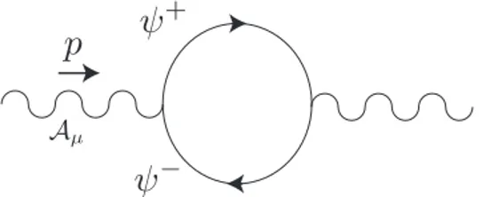
Figure 2. Fermion contribution to the vacuum polarization.
expressions of the propagators onR3×S1 in the presence of a non-trivial holonomy. Both of these topics are summarized in appendixA.
The adjoint Dirac fermions couple to the holonomy A3, the dynamical gluon am, and the background field Am as
L= Z
d4xψ¯aγm
∂mδac+fabcAb3δ3m+fabcabm+fabcAbm
ψc, (3.8)
from which one can easily read the fermion-background field vertex:
gfabc=−ig(Tadjb )ac. (3.9) Then, using the propagator (A.8), the one-loop fermion contribution to the vacuum polar- ization for any gauge group reads (see figure 2)
ΠDedmn (p, ω) =−g2 L
X
q∈Z
Z d3k (2π)3Tradj
TeTdγm
1 K/γn
1 K/ +P/
(3.10)
=−4g2 L
X
q∈Z
tradj
Z d3k (2π)3
TeTd
δmn −K·P −K2
+KmPn+KnPm+ 2KmKn
k2+ 2πq
L +Ab3Tb 2
(kkk+ppp)2+ 2πq
L +Ab3Tb+ω 2
.
where the superscript D denotes that the expression is given for a single Dirac fermion, Tr denotes the trace over both the color and gamma matrices, K·P = k0 ·p0 +kkk·ppp, K2 =k20+k2,k0= 2πnL +Ab3Tb, and p0 =ω.
One can also use the background field method in the Cartan-Weyl basis by turning on background fields along the Cartan generators Am =AimHi. In this case, one can derive the fermion-background field vertex simply by replacingβiφi with βiAiµ in (A.14). Thus, we find the fermion-background field vertex:
gβiAiµ. (3.11)
Then, we use the propagator (A.15) to find the vacuum polarization in the Cartan-Weyl basis:
ΠDmnij =−4g2 L
X
β β β
X
q∈Z
Z d3k (2π)3
βiβj
gmn −K·P −K2
+KmKn+KnPm+ 2KmKn
k2+ 2πq
L +φ2πLiβi 2
(kkk+ppp)2+ 2πq
L +φ2πLiβi +ω 2 .
(3.12)
JHEP01(2015)139
In order to simplify the calculations, we take G=su(N) and perform our analysis at center-symmetry. The value of the holonomy in the center-symmetric case is given by (3.7).
In addition, forN = 2,3 one can easily see that the combination 2πn+ρL iβi falls into one of two categories: either 2πn+µL or 2πn−µL ,18 where
µ= 2π
N , N = 2,3. (3.14)
Therefore, for su(2) andsu(3) the vacuum polarization tensor takes the form ΠDijmn = −4g2
L X
β β β(1)
X
q∈Z
Z d3k (2π)3
βiβj
δmn −K·P −K2
+KmPn+KnPm+ 2KmKn
k2+
2πq+µ L
2
(kkk+ppp)2+
2πq+µ L +ω
2
−4g2 L
X
ββ β(2)
X
q∈Z
Z d3k (2π)3
βiβj
δmn −K·P −K2
+KmPn+KnPm+ 2KmKn
k2+2πq−µ
L
2
(kkk+ppp)2+2πq−µ
L +ω2 ,
where βββ(1,2) denotes the roots in the first or second category. Now using P
βββ(1,2)βiβj = δµνN/2 (keeping in mind that N = 2,3 only), we finally obtain
ΠDmnij(p, ω) = −δµν4N g2 2L
X
q∈Z
Z d3k (2π)3
δmn −K·P−K2
+KmPn+KnPm+ 2KmKn
k2+
2πq+µ L
2
(kkk+ppp)2+
2πq+µ
L +ω2
+(µ→ −µ). (3.15)
It is easy to understand the physics behind the simplified formula (3.15) forN = 2,3 since in these cases all charged fermionsψβββ have exactly the same mass in the center-symmetric vacuum. For N >3 the charged fermions will generally have different masses, and hence one has to restore to the original expressions (3.10) or (3.12).
In fact, one can obtain the result (3.15) directly from (3.10) for N = 2,3 by setting Ab3Tb =±µ/Land using Tradj[TeTd] =fadcfcea=N δed. This is a huge simplification since one can then use the same background field Feynman rules, as given by Abbott [32], to compute the non-abelian one-loop corrections onR3×S1, shown in figure3, provided that we substitute the ghosts and gluons propagators on R4 with the propagators on R3×S1
18This is trivial to see insu(2) since there are only two rootsβββ1,2=±1. Thesu(3) case requires a bit more work. The roots, fundamental weights, and Weyl vector are given by
ββ
β1 = (1,0), βββ2=
−1 2,
√3 2
, βββ3=
−1 2,−
√3 2
, β
β
β4 = (−1,0), βββ5= 1
2,−
√3 2
, βββ6=
1 2,
√3 2
, ωωω1 =
1, 1
√3
, ωωω2=
0, 2
√3
, ρρρ= 1,√
3
. (3.13)
Then, we find 2πρρρ·βββ1/N = 2π/3, 2πρρρ·βββ2/N = 2π/3, and 2πρρρ·βββ3/N =−4π/3. We see that theses values belong to the first category given that we shiftn→n+ 1 in 2πn+ρLρρ·βββ3. Similarly, we find that the values 2πρρρ·βββ4/N =−2π/3, 2πρρρ·βββ5/N =−2π/3, and 2πρρρ·βββ6/N = 4π/3 belong to the second category after making the shiftn→n−1 in 2πn+ρLρρ·βββ6.
JHEP01(2015)139
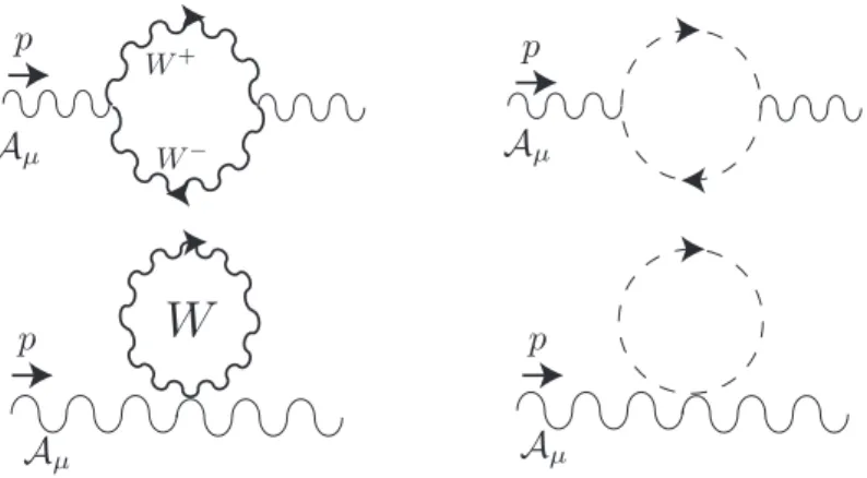
Figure 3. Diagrams contributing to the non-ableian part of the vacuum polarization (3.16). The dashed lines are the ghosts, and that the second line of diagrams does not contribute on R4 in dimensional regularization.
in the presence of a non-trivial holonomy. The diagrams of figure 3(for N = 2,3) add up to [33]:
ΠN A ijmn (p, ω) =δijg2N 2L
X
q∈Z
Z d3k (2π)3
×4δmnP2+ 2 (PmKn+PnKm) + 4KmKn−3PmPn−2(K+P)2δmn
k2+
2πq+µ L
2
(kkk+ppp)2+
2πq+µ
L +ω2
+ (µ→ −µ). (3.16)
Before proceeding to the the computation of the expressions (3.15) and (3.16), we review the procedure for summing up an infinite number of bubble diagrams.
3.3 The general form of the gluon propagator
In this subsection, we briefly review the procedure to sum an infinite number of bubble diagrams. The Euclidean bare gluon propagator in the Feynman gauge on R3 ×S1 takes the form
Dab ,0mn = δabδmn
p2+ω2, (3.17)
where a, b are the color indices. The vacuum polarization is defined as the difference between the inverse full gluon propagator and the inverse bare gluon propagator:
Πabmn=D−1mnab ,0−Dmn−1ab. (3.18) Assuming that the polarization tensor is diagonal in the color indices, we can write the polarization tensor in the general form
Πabmn =δabΠmn=δab FPmnL +GPmnT
, (3.19)
JHEP01(2015)139
where the projection operators PmnT and PmnL are defined as P33T =P3µT = 0, PµνT =δµν−pµpν
p2 , PmnL =δmn− PmPn
p2+ω2 − PmnT . (3.20) The projection operators obey the usual relationsPTPT =PT,PLPL=PL, andPTPL= 0. Next, one uses the fact that the polarization tensor is transverse,PmΠmn= 0, to express Π33 as
Π33= pµpµΠµν
p23 . (3.21)
Then, we set m=n= 3 and m=n=µin (3.19), to obtain F =
1 +ω2
p2
Π33, G= 1 2
Πµµ−ω2 p2Π33
. (3.22)
One can therefore express the full polarization tensor as a function of Π33and Πµµ. Notice that in order for theF and G functions to be non-singular, the Π33 must vanish asp2 for nonzeroω. This will be one check of our results given in (4.16). Finally, one can sum the polarization tensor to obtain the full propagator
Dmnab =δab
1
p2+ω2−GPmnT + 1
p2+ω2−FPmnL
. (3.23)
As we will see in section 5, the full propagator on R3×S1 in the presence of a non-trivial holonomy does not suffer from any IR logarithmic singularity, and hence QCD(adj) on a compact circle is an IR renormalon free theory.
4 Calculating the polarization tensor on R3 ×S1
In this section, we compute the one-loop contribution from fermions and gauge bosons as given by (3.15) and (3.16). All the excited Kaluza-Klein modes cannot causeIRproblems as they have a Matsubara mass, and all infrared singularities, if any, will show up in the static limit ω = 0. Before taking the static limit, we compute the total polarization for QCD(adj) as a general function ofpand ω. We postpone the discussion of the static limit to the next section.
4.1 The one-loop fermion correction
The fermions contribution to the vacuum polarization is given by (3.15) (see figure 2).
Keeping in mind that this expression is given for a single Dirac fermion, and ignoring the color indices, we find that the contribution from nW Weyl fermions is given by the expression
ΠWmn = nW 2 ΠDmn.
JHEP01(2015)139
Before proceeding to the calculations of (3.15), we first examine the limitL→ ∞. Making the replacement
1 L
X
n∈Z
Z d3k (2π)3 →
Z d4K
(2π)4, (4.1)
and performing the calculations using the dimensional-regularization method, by substi- tuting 4→D= 4−, we obtain
ΠL→∞mn (P) =−2nWN g2
3 (4π)2 (P2δmn−PmPn) logP2, (4.2) where we have ignored the 1/ piece accompanying the logarithm which can be absorbed in a counter term. The expression (4.2) is the standard background field textbook result in four dimensional field theory.
Now, we turn to the full calculation of (3.15). First, one needs to sum over the Kaluza- Klein modes. Such sums can be performed with the help of the complex plane and the residue theorem. In appendix (B), we summarize and compute the list of the sums we encounter in this paper. Among the sums we denote by S0, S1, S2, and S3, only S0 and S1 are independent. In terms of S0, S1, and S2 the Π33 and Πµµ components of the polarization tensor read:
ΠWµµ = −2nWN g2
Z d3k (2π)3
−kkk·ppp+ 2k2
S1−3ωS2−3S0 , ΠW33 = −2nWN g2
Z d3k (2π)3
−kkk·pppS1−2k2S1+S2ω+S0
. (4.3)
The structure of the sums S1 toS3, which appear in appendix (B), takes the general form S= Re
1 epL−iµ−1
F(pL, ωL) +1
2F(pL,−ωL), (4.4) where F depends on the specific details of the sum. The first term in (4.4) is the contri- bution from the µ-dependent part of the sum, while the second term is the vacuum part, L→ ∞. We see that the µ-dependent term can be obtained from the vacuum part upon replacing 12 → Reh
1 epL−iµ−1
i
and ω → −ω . This observation will prove to be crucial for the cancellation of the IR divergences as we explain below.
Using the integrals in appendix C, we can express the polarization tensor in terms of the integralsI0,I1,I2, and I3:
ΠWµµ = −2nWN g2 L2
−
1 +2ωL pL tan−1
pL ωL
I0+
p2L2
2 +ω2L2 2
I1
+4I2+ 2ωLI3
, (4.5)
and
ΠW33 = −2nWN g2 L2
−
1−2ωL pL tan−1
pL ωL
I0+
p2L2
2 +ω2L2 2
I1
−4I2−2ωLI3
. (4.6)
JHEP01(2015)139
The integralsI0 toI3 result from integrating the sumsS0 toS3 overk. Inheriting the sum structure, the IR behavior of these integrals can be studied by casting the integrals in the following form:19
I =IV +δI = Z
0
dx 1
2 + Re
1 ex−iµ−1
G(pL, ωL, x), (4.7) where the function G(pL, ωL, x) depends on the details of the integral. The first part of (4.7), G(pL, ωL, x)/2, is the vacuum contribution to the integral, while Re
1 ex−iµ−1
G(pL, ωL, x) is theµ-dependent contribution.
Now, we discuss a general feature of the integral (4.7) which is vital for the absence of the infrared renormalons. The integral R
dxG(pL, ωL, x)/2 has an IR logarithmic divergence:
IV = limq→0
Z
q
dxG(pL, ωL, x)
2 = N
2 logP +. . . , (4.8) whereP =p
p2+ω2,N is some number that depends on the explicit form ofG, and the dots represent terms that are not singular in the IR. On the other hand, the µ-dependent part in (4.7) suffers from the same IR divergence which can be extracted by expanding Re
1 ex−iµ−1
about x= 0: Re 1
ex−iµ−1
∼=−12 +O(x). Thus, we find
δI = limq→0
Z
q
dxRe
1 ex−iµ−1
G(pL, ωL, x) (4.9)
= −limq→0 Z
q
dxG(pL, ωL, x)
2 +. . .=−N
2 logP +. . . . (4.10) Comparing (4.8) with (4.10), we see that the IR parts cancel as we add IV to δI. This cancellation can also be seen immediately by computing the integrals δI0 to δI3. To the best of our knowledge, these integrals are not known in the literature. In appendix E, we use a novel method to compute the integrals. We list the final expressions of I0 to I3 in appendixD. From the explicit form of these integral, we find that the logarithms that come from the lower limit of the vacuum integrals IV cancel exactly with the corresponding logarithmic dependence of δI.
4.2 The non-abelian part of QCD one-loop correction
In this subsection, we repeat the same analysis we carried out above for the non-abelian case. At infinite circle radius we obtain from (3.16)
ΠN A ,L→∞mn (P) = 11g2N
3(4π)2(P2δmn−PmPn) logP2, (4.11) thus we have the famous QCD β-function coefficient.
19We stress that this form is appropriate only to study the IR behavior of the integrals and to show the cancellation of the logarithms between the vacuum and the volume dependent parts.