engineering
A. Oschlies1, H. Held2, D. Keller1, K. Keller3,4, N. Mengis1, M. Quaas5, W. Rickels6, and H. Schmidt7
1GEOMAR Helmholtz Centre for Ocean Research Kiel, Research Division Marine Biogeochemistry, Germany,2Center for Earth System Research and Sustainability (CEN), University of Hamburg, Germany,3Department of Geosciences, Penn State University, University Park, Pennsylvania, USA,4Department of Engineering and Public Policy, Carnegie Mellon University, Pittsburg, Pennsylvania, USA,5Department of Economics, Kiel University, Germany,6Kiel Institute for the World Economy, Research Area The Environment and Natural Resources, Germany,7Max Planck Institute for Meteorology, Department The Atmosphere in the Earth System, Hamburg, Germany
Abstract
Selecting appropriate indicators is essential to aggregate the information provided by cli- mate model outputs into a manageable set of relevant metrics on which assessments of climate engineer- ing (CE) can be based. From all the variables potentially available from climate models, indicators need to be selected that are able to inform scientists and society on the development of the Earth system under CE, as well as on possible impacts and side effects of various ways of deploying CE or not. However, the indicators used so far have been largely identical to those used in climate change assessments and do not visibly reflect the fact that indicators for assessing CE (and thus the metrics composed of these indicators) may be different from those used to assess global warming. Until now, there has been little dedicated effort to identifying specific indicators and metrics for assessing CE. We here propose that such an effort should be facilitated by a more decision-oriented approach and an iterative procedure in close interac- tion between academia, decision makers, and stakeholders. Specifically, synergies and trade-offs between social objectives reflected by individual indicators, as well as decision-relevant uncertainties should be considered in the development of metrics, so that society can take informed decisions about climate pol- icy measures under the impression of the options available, their likely effects and side effects, and the quality of the underlying knowledge base.1. Introduction
When the scientific and societal debate about climate engineering (CE) was only beginning, as was the case when theCrutzen[2006] paper was written, the assessment of CE was based on climate indicators that had already been used in climate-change assessments [e.g.,Nordhaus, 1992]. WhileCrutzen[2006] discussed the radiative forcing from hypothetical stratospheric sulfur injections and its effect on global-mean surface air temperature, already in his brief essay he mentioned possible damages of the ozone layer—implicitly sug- gesting stratospheric ozone levels as a further indicator of possible relevance for CE measures that consider aerosol injections into the high atmosphere. He also mentioned possible trade-offs between aerosol injec- tions into the stratosphere versus injections into the troposphere in terms of amounts and residence times of injected aerosols, the radiative cooling, and possible environmental side effects. This already hinted at the intricacies of comprehensively assessing CE, for which traditional (albeit still improvable) assessment methods used in the context of global warming may not be fully sufficient. Here, we explore to what extent indicators and metrics need special consideration with respect to assessing CE, so that society can take an informed decision about CE under the impression of likely effects and side effects and the quality of the underlying knowledge base. Examining assessment methods in the context of CE may also help to further improve the tools appropriate for assessing climate change.
Any quantitative assessment of possible consequences of CE requires indicators and corresponding metrics to measure the CE-induced changes in the (simulated) Earth system and their impacts on natural and human systems. Indicators are measureable variables that describe the Earth system, including human activities.
Metrics are functions that quantify the distance of one or more indicator values from some reference level in terms of a single or manageably small number of measures. Indicators and metrics are usually used by scien- tists to quantitatively analyze impacts of climate change or CE on the Earth system and by decision makers 10.1002/2016EF000449
Special Section:
Crutzen+10: Reflecting upon 10 years of geoengineering research
Key Points:
• Traditional climate change indicators and metrics may lose their relevance under climate engineering (CE)
• A comprehensive assessment of CE and mitigation would benefit from common indicators and metrics
• We propose an iterative process between scientists and stakeholders to define indicators and metrics for assessing CE
Supporting Information:
• Supporting Information S1
Corresponding author:
A. Oschlies, aoschlies@geomar.de
Citation:
Oschlies, A., H. Held, D. Keller, K. Keller, N. Mengis, M. Quaas, W. Rickels, and H.
Schmidt (2016), Indicators and metrics for the assessment of climate engineering,Earth’s Future,5, doi:10.1002/2016EF000449.
Received 30 AUG 2016 Accepted 8 NOV 2016
Accepted article online 14 NOV 2016
© 2016 The Authors.
This is an open access article under the terms of the Creative Commons Attribution-NonCommercial-NoDerivs License, which permits use and distri- bution in any medium, provided the original work is properly cited, the use is non-commercial and no modifica- tions or adaptations are made.
to negotiate trade-offs between different social objectives and possible options for action, for example, via integrated assessment frameworks. Examples of indicators employed in the context of climate change include global-mean surface air temperature (GMST), sea level, atmospheric CO2concentrations, human life expectancy, economic productivity, or welfare. Indicators often describe larger-scale spatial and/or tem- poral longer averages, but can also refer to local properties and statistical extremes. A metric aggregates values of these indicators into a single or very few composite measures. Metrics used in the assessment of climate change and CE include the distance of climate indicator values like surface air temperature rel- ative to pre-industrial levels or to defined “planetary boundaries” that have been proposed to define a safe operating space for humanity [Rockström et al.,2009], or damages estimated, for example, based on quadratic normalized differences of regional temperature and precipitation from some reference state [e.g., Moreno-Cruz et al., 2012]. Studies differ in the adopted metric for climate change or for CE, in part because different actors, different environmental conditions, and different scenarios may require different metrics [e.g.,Irvine et al.,2012].
Historically, assessments of climate change, in particular the assessment reports of the Intergovernmental Panel for Climate Change [IPCC;Pachauri et al.,2014], have helped to establish GMST as the most widely used indicator for the state of the climate system. A corresponding single-indicator metric is the difference in GMST with respect to pre-industrial levels. Integrated assessment models often rely on this metric to project damage costs associated with climate change that enter the economic models [e.g.,Hope et al.,1993;
Nordhaus, 1993;Tol, 1997;Stern, 2006], and the United Nations Framework Convention on Climate Change, including the recent Paris agreement, formulate their climate mitigation targets by means of this metric [United Nations Framework Convention on Climate Change (UNFCCC), 2015]. The widespread use of GMST may be justified by the fact that many physical climate indicators are correlated with GMST, for example, evapo- ration, precipitation, sea level, and even extremes in temperature and precipitation [Seneviratne et al., 2016].
As discussed bySutton et al.[2015], these correlations differ with the indicator considered, and depend on the spatial and time scales of interest, and the type of forcing that causes the GMST change, an issue of particular relevance for some forms of CE.
2. Indicators Used in Climate Engineering Research
Individual modeling studies of the climate resulting from hypothetical implementation of solar radiation management (SRM) had already been performed prior toCrutzen’s[2006] paper [e.g.,Govindasamy and Caldeira, 2000]. In recent years, multi-model SRM studies followed within the framework of the Geoengi- neering Model Intercomparison Project [see, e.g.,Kravitz et al.[2013a] and references therein), and a Carbon Dioxide Removal Model Intercomparison Project is just starting (www.kiel-earth-institute.de/CDR_Model_
Intercomparison_Project.html). One may broadly distinguish two categories of indicators used in such stud- ies: (1) indicators that help to characterize the climate, be it quantities that can be thought to be relevant for impacts (e.g., global and regional temperature or precipitation, e.g., Schmidt et al., 2012) or quantities of rather academic interest (e.g., components of the planetary energy budget, e.g.,Niemeier et al.,2013) and (2) indicators that characterize impacts of climate change like crop yield [Xia et al., 2014] or the Gross Domes- tic Product [GDP;Aaheim et al.,2015]. The latter group of indicators is typically not a direct climate model output but requires additional impact modeling or assessment. Indicators of the former group have often been chosen with the potential relevance for impacts in mind. For example, regional temperature and pre- cipitation changes can impact people’s lives. Damages may result rather from extremes than means of these quantities and hence extremes have also been used as indicators [e.g.,Curry et al.,2014]. Similarly, besides pure precipitation, indicators like the Bowen ratio [e.g.,Schmidt et al., 2012] or potential evapotranspiration [Kristjánsson et al.,2015] that are considered more relevant for aridity and hence vegetation have been used.
The breakdown of correlations between GMST and other climate indicators under SRM has at least implic- itly been acknowledged in these studies. Many studies have addressed simulations where greenhouse-gas radiative forcing is, on a global average, exactly balanced by SRM. In these scenarios GMST remains constant, but changes are simulated, e.g., in global-mean precipitation and regional temperatures.
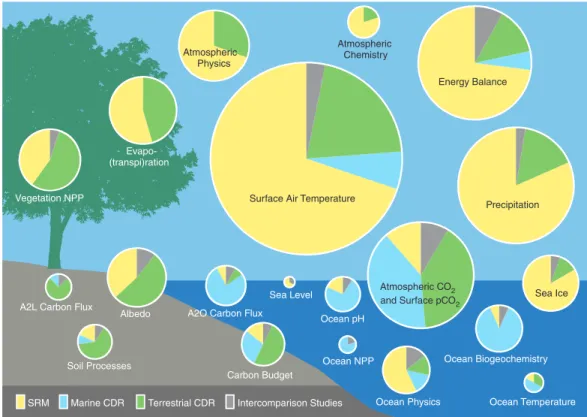
Results of an exhaustive literature survey shown in Figure 1 indicate that the three most often used indica- tors to assess CE are, until now, GMST, the planetary energy budget, and precipitation (most of these studies have investigated SRM, Figure 1; see also Table S1, Supporting Information). Other indicators describing properties related to the atmosphere, the hydrological cycle, vegetation, or sea ice were frequently used as
Surface Air Temperature Evapo-
(transpi)ration
Precipitation Vegetation NPP
Atmospheric Physics
Atmospheric CO2 and Surface pCO2
Energy Balance Atmospheric
Chemistry
Albedo
Sea Ice
Ocean Temperature Carbon Budget
SRM
Ocean pH
Ocean Physics
Ocean Biogeochemistry Sea Level
Ocean NPP Soil Processes
A2L Carbon Flux
A2O Carbon Flux
Marine CDR Terrestrial CDR Intercomparison Studies
Figure 1.Results of a literature survey of climate engineering studies investigating solar radiation management (SRM, yellow), terrestrial carbon dioxide removal (CDR, green) and marine CDR (blue). Studies that investigate various methods are shown in gray. The size of each circle refers to the number of studies that used the respective indicator (ranging from 3 for sea level to 64 for surface air temperature), colors indicate the relative proportion of the studies referring to the specific classes of CE method(s). Indicators are located approximately in the physical space they refer to.
well. Sea level has, until now, been used as indicator in relatively few studies, even though it is often con- sidered as one of the major threats associated with global warming. In the long-term (but not necessarily during periods of decreasing radiative forcing [Bouttes et al.,2013]), sea level is normally found to be closely correlated with GMST, and so far there have been no reports that this correlation should change under CE.
Investigations of marine carbon dioxide removal (CDR) techniques have looked mostly at oceanic and atmo- spheric carbon, e.g., air–sea CO2fluxes, and marine biogeochemistry. In contrast, as can also be seen from Figure 1, investigations of terrestrial CDR techniques have put an emphasis on indicators describing veg- etation, albedo, evapotranspiration, as well as fluxes of CO2and water, predominantly between land and atmosphere. Thus, individual CE methods have primarily been investigated by means of different indica- tors, and hence a common metric would be difficult to establish from these studies. Joint sets of indicators for different CE methods, which would be required to evaluate these methods against each other, have been used by only few studies until now [Lenton and Vaughan, 2009;Vaughan and Lenton, 2011;Keller et al., 2014]. Overall, the indicators used have been largely identical to those used in climate change assessments and do not visibly reflect the fact that indicators for assessing CE (and thus the metrics composed of these indicators) may be different from those used to assess global warming.
3. Special Requirements for CE Indicators?
We argue that the requirements for CE indicators and the corresponding metrics differ from those already used to assess mitigation of climate change for at least two reasons:
1. CE can change the correlations between different climate variables [Sutton et al.,2015]. In particular under SRM, atmospheric CO2levels and GMST do not need to remain positively correlated. Other examples include alterations in the correlation between atmospheric CO2and GMST by afforestation or artificial ocean upwelling [Keller et al.,2014;Mengis, 2016]. Thus, single indicators such as GMST or atmospheric CO2may have less explanatory power in describing an engineered than a non-engineered
climate state. Therefore, indicators required to comprehensively describe the state of an engineered climate system may differ from those that can describe the state of the system without CE.
2. Effects to be assessed in the context of CE concern both the intended effects of CE as well as unintended side effects and their potential impacts on society. Because of the different legal and ethical issues regarding intentional versus unintentional interventions, an assessment of side effects and their causalities will likely be more important for an intentional manipulation of the climate system than for “unintentional” global warming resulting from greenhouse-gas emissions. Responsible assessments will also have to consider possible intergenerational impacts [Goeschl et al.,2013] and hence may include longer timescales than normally considered in climate-change assessments. With carbon dioxide avoidance or removal options becoming widely available, calling global warming by unabated emissions of CO2“unintentional” will become more and more problematic, and this differences between assessing CE and global warming may disappear.
Metrics require a reference state for any of the selected indicators. Global warming studies usually refer to some observed historical (e.g., pre-industrial) or present climate. In CE studies, the appropriate reference state becomes less obvious. The pre-industrial situation, defined by the IPCC as the period prior to year 1750, has often been used in assessments of CE, where the target of CE is to reach a state closer to the pre-industrial reference than that of a climate without CE [Kravitz et al.,2014a]. Whether, or for how long, such a reference state remains appropriate under ongoing climate change is an open question that needs further investi- gation. Some CE studies [e.g.,Goes et al., 2011] have also employed future hypothetical climate states from scenarios without CE as reference states.
It is perhaps trite to state the metrics to assess CE should be decision relevant and reflect important concerns of stakeholders and decision makers (see, e.g.,Radermacher[2005] on indicator selection), where stake- holders and decision makers may often but not always be the same actors, e.g., not all stakeholders may have a voice in the decision-making process. Until now, there has been little dedicated effort to establish specific metrics for assessing CE. Within the German Research Foundation-funded Priority Program on the Assessment of CE (SPP 1689, www.spp-climate-engineering.de) we have initiated discussions about the development of metrics appropriate for a comprehensive assessment of CE. We outline the current state of these ongoing discussions below.
4. Approaches for Selecting Indicators
Any quantitative assessment has to deal with the selection of appropriate indicators that can be aggre- gated into a metric that measures net benefit or harm of individual CE and mitigation approaches. Against the background of large uncertainties about the state and sensitivity of the climate system, and given the absence of historical analogs of engineered climates, no unambiguous rules for indicator selection have been established. In the following, we identify three main approaches to select CE indicators.
4.1. Bottom-Up Approaches
Bottom-up approaches are based on a scientific investigation of the Earth system yielding a descriptive set of indicators. Statistical procedures can support the selection of indicators among the set of measurable variables of the climate system into a subset of indicators that explain most of the variance. One recent example of such an approach in the context of CE exploits correlations between various measurable Earth system variables across simulations of different CE and mitigation scenarios, multi-model ensembles, or per- turbed parameter ensembles [Mengis, 2016]. Analysis of these correlations allows the identification of rela- tively small sets of indicators ranked by the number of significant correlations with other variables except for already selected indicators. These indicators can explain most of the expected variance of the impact of sim- ulated CE deployments on all Earth system variables, while avoiding double counting of individual impacts via correlated indicators. This approach ensures measurability, but not necessarily societal relevance of the selected set of indicators. Future research on bottom-up approaches is needed to clarify a number of open questions: First, also a bottom-up approach includes normative choices, specifically with regard to the con- struction of the set of measurable earth system variables from which the indicators are chosen, and the significance level of the statistical correlations that enters the analysis. Methods to make these normative choices explicit and transparent need to be found. Second, correlations and thus selected indicators can vary across different CE methods and also different background climate states. Yet, it may be possible to find
general indicators that are at the same time appropriate for different scenarios. Third, extremely nonlinear metrics, e.g., considering thresholds, may require going beyond linear correlation analysis when construct- ing an appropriate set of indicators.
Since some indicators identified via this bottom-up approach may have relatively little political relevance, it is possible to include “expert judgment” by prior selection of a few indicators and then complementing them by additional indicators that are uncorrelated with the pre-selected ones. Selecting a few indicators via scientific expert judgment and complementing these by indicators derived from a correlation analysis introduces normative choices, but can still allow most of the expected signal variance to be explained while avoiding double counting.
4.2. Top-Down Approaches
This approach is driven by the overarching question of what is needed for decision making, i.e., it starts from the selection criterion of societal relevance, while ensuring measurability. One of the most ubiquitous metrics in economics is the GDP, which is a top-down approach of aggregating individual economic val- ues into one overarching metric (usually taking the previous year’s GDP as the reference level). The idea is that key effects that are relevant for human welfare can be approximately expressed in monetary terms, and aggregated into some augmented version of GDP as the unique metric of human well-being. While in a hypothetical perfect economy all values are captured by markets [Weitzman, 1976], the approach can be extended in many ways to take welfare effects into account that are not captured by market transac- tions in actual economics. This is the idea, for example, in the comprehensive wealth approach [Arrow et al., 2003]. Obviously, such extensions of the traditional GDP metrics are needed to capture all welfare-relevant effects of CE. Damages of climate change are usually assumed to depend on GMST only (or the rate of GMST change, seeGoes et al. [2011]). Other indicators such as frequency or intensity of heat waves, regional pre- cipitation, precipitation extremes, Arctic summer sea ice extent, or measures of ocean acidification have been regarded as societally relevant and used, for example, in the IPCC’s summary for policymakers [Inter- governmental Panel for Climate Change,2013]. Yet, today it remains questionable whether it is feasible to aggregate all relevant climate effects into a single or very few composite indicators (e.g., GMST or conversion into monetary units). On the other hand, different societally relevant indicators may be closely correlated via physical and/or biogeochemical processes in the climate system, though correlations may be different for different deployments of CE. This may lead to double counting of some effects of some CE methods if multiple indicators are used in the assessment.
4.3. Iterative Approaches
Climate indicators identified via the bottom-up approach discussed above are—by design—of interest to scientists. The indicators identified by the top-down approach are designed to be decision relevant. These two approaches can provide different perspectives that each are useful for themselves. Still, the selection of indicators that are published represents a value-loaded process as it implies that the set of published indicators captures all information that is relevant for the evaluation. One could argue that indicators for a societally relevant assessment of CE should eventually be selected by society. However, the plethora of potential candidates for indicators would imply too large a burden in terms of its complexity for direct selec- tion by decision makers who are not trained climate scientists. To address this challenge, academics can make suggestions for indicator selection (ensuring measurability of indicators), elicit what categories of effects would matter at all for stakeholders (bringing in the criterion of societal relevance [de la Vega-Leinert et al., 2008]), and iteratively account for feedback from stakeholders [Welp et al.,2006] and decision makers in the process of suggesting revised indicators.
Specifically, a number of indicator-related questions intrinsically require interactions between scientists, decision makers, and stakeholders. For example, are the selected indicators salient to the objectives of stakeholders and decision makers? What are the most decision-relevant uncertainties as a function of the different objectives, and do the indicators and scenarios sample these uncertainties? How does the choice and presentation of the indicators and trade-offs and the associated uncertainties impact decision making?
What are the preferences of stakeholders and decision makers after they have seen key trade-offs between their objectives? Methods and approaches developed in the areas of robust decision making, decision anal- ysis, and judgment and decision making combined with an iterative approach can help to address these questions (see, e.g.,Hall et al.[2012];Hamarat et al.[2013];Kasprzyk et al. [2013];Edenhofer and Kowarsch
[2015];Hadka et al.[2015];Singh et al.[2015];Garner et al.[2016], who emphasize the role of iteration for refining value system in view of systemic boundary conditions).
Iterative approaches will prove key to indicator selection. Academia and society would share their inputs for generating solution scenarios that they legitimately can bring in: society can provide preferences on values, academia can provide systemic trade-offs and boundary conditions. However, in practice this cannot be a mere addition, as society might be unaware of systemically intricate trade-offs that only academic advice can reveal. For example, might society revise a global-mean temperature target (in either direction) once it learns that according to current scientific understanding and in contrast to the situation in the 1990s, the 2-degree target implied the usage of carbon capture and storage (CCS) or even CE, or that certain low-lying island states might be lost? Would the accounting of carbon sequestered via afforestation be viewed differ- ently when radiative forcing of afforestation was found to lead to a net warming? Hence, under progressing climate change and improving scientific understanding society might learn about trade-offs or synergies.
Thereby it would develop a more refined version of its preference order under the impression of the most recent version of scientific solution scenarios. Academia, in turn, might have been unaware or ignorant of preferences and might therefore want to augment their set of indicators and of solution scenarios in the discourse with society.
To our impression, this iterative concept readily applies for indicator selection. For mitigation, a global-mean temperature target might have been enough to be traded off against present costs of mitigating greenhouse-gas emissions. However, society now has to deal with the fact that under the still hypo- thetical usage of CE (and arguably already under climate change without CE [Seneviratne et al.,2016]), GMST may cease being a good indicator for regional climate and might have to be replaced by regional targets. This might be a moment where new choices of indicators and, eventually, metrics might have to come in. To optimize this iterative selection of indicators and their eventual aggregation into metrics, other disciplines in addition to natural sciences should be engaged.
5. Recommendations for Future Research
A comprehensive assessment of CE in the context of mitigation will benefit from common assessment met- rics that, in turn, will be based on common indicators. As a first step to developing appropriate common metrics, we need to identify the appropriate indicators relevant for the assessment of CE and climate change.
Selecting appropriate indicators, and dropping others, will be essential to aggregate the information pro- vided by climate model outputs into a manageable set of relevant measures. The selection of indicators is thus not only at the heart of developing a comprehensive assessment of CE, it is also important for scenario development and the analysis of scenario simulations. Addressing these questions should be facilitated by a more decision-oriented approach (in contrast to the perhaps more straight-forward emission-scenario driven approaches in climate change research) and tighter trans-disciplinary collaboration. We believe that this can be approached best in an iterative procedure in close interaction between academia and society.
In particular, we need to improve our understanding about trade-offs between different social objectives across space and time, and also about the decision-relevant uncertainties.
Some societally relevant indicators may not be easy to quantify with current tools. This applies in particu- lar for possible impacts of CE on society. The information about such indicators may well be essential for future decisions about CE. This raises the, thus far, open questions: (1) How could such indicators be con- structed? (2) How could their uncertainties be estimated? (3) How can stakeholders, society and scientists inform each other about issues relevant for decision making? Again, this may work best in an iterative pro- cedure involving both, scientists with different disciplinary backgrounds and various stakeholders. As a first step to achieve this, scientists must ensure that their work is transparent and publicly accessible, but active approaches to engage with stakeholders and policymakers in joint workshops and exchanges of ideas have to be included in the research plan.
Appendix
A1 Database Acknowledgments
We would like to acknowledge the following sources used to generate Figure 1:Akbari et al.[2012],Bala et al. [2008],Brovkin et al.[2009], Ferraro et al.[2014],Heckendorn et al.[2009],Irvine et al.[2011, 2014],
Acknowledgments
The authors thank the DFG for fund- ing the Priority Program SPP 1689. The unselfish effort of the many colleagues who helped to initiate this activity and move it along as a science-driven com- munity effort is specifically acknowl- edged. This work was also partially supported by the National Science Foundation through the Network for Sustainable Climate Risk Management (SCRiM) under NSF cooperative agree- ment GEO-1240507. Any opinions, find- ings, and conclusions or recommen- dations expressed in this material are those of the author(s) and do not nec- essarily reflect the views of the National Science Foundation. We thank Rita Erven for help with the graphics and two reviewers for their constructive comments that helped to improve the manuscript. The data used in this study are from the cited references.
Kleidon and Renner[2013],Kleidon et al. [2015],Kravitz et al.[2013b],MacMartin et al.[2014],Matthews and Caldeira[2007],Niemeier et al.[2013],Ross and Matthews[2009],Schaller et al.[2014],Berdahl et al.
[2014],Huneeus et al.[2014],Jones et al.[2013],Kravitz et al.[2014b],Schmidt et al.[2012],Govindasamy and Caldeira[2000],Govindasamy et al.[2002, 2003], Bala et al.[2011],Caldeira and Wood[2008],Kravitz et al.
[2012],Lunt et al.[2008],Matthews et al.[2009],Rasch et al.[2008, 2009],Ricke et al.[2010],Robock et al.
[2008],Tilmes et al.[2009],Pongratz et al.[2012],Cvijanovic et al.[2015],Muri et al.[2015],Tilmes et al.[2014], Xia et al.[2014],Kuebbeler et al.[2012],MacMartin et al.[2013],Ban-Weiss and Caldeira[2010],Doughty et al.
[2011],Ridgwell et al. [2009],Applegate and Keller[2015],Irvine et al.[2012],Tjiputra et al.[2016],Harvey [2008],Oschlies[2009],Oschlies et al.[2010a, 2010b],Kwiatkowski et al.[2015],Arora and Montenegro[2011], Ornstein et al.[2009],Betts[2000],Bathiany et al.[2010],Arora et al.[2013],Davies-Barnard et al.[2014],Sitch et al.[2005],Sonntag et al.[2016],Wang et al.[2015],Claussen et al.[2001],Tokimatsu et al.[2016],Keller et al.
[2014],Vaughan and Lenton[2011],Fyfe et al.[2013],Naik et al.[2003],Heck et al.[2016],Brovkin et al.[2013], Pongratz et al.[2011],Zeebe and Archer[2005],Hangx and Spiers[2009],Heimann[2014],Ilyina et al.[2013], Vichi et al.[2013],Aumont and Bopp[2006],Sarmiento and Orr[1991],Cao and Caldeira[2010],Caldeira and Rau[2000],Cripps et al.[2013],House et al.[2002],Lenton and Vaughan[2009],Niemeier et al.[2011],Tilmes et al.[2008],Jin and Gruber[2003],Kirschbaum et al.[2011],Moore et al.[2010],Seidel et al.[2014],Smith [2016],Gnanadesikan et al.[2003],Smith and Torn[2013],Couce et al.[2013],Yool et al.[2009],Köhler et al.
[2013],Rau[2008],Kato and Yamagata[2014].
References
Aaheim, A., B. Romstad, T. Wei, J. E. Kristjánsson, H. Muri, U. Niemeier, and H. Schmidt (2015), An economic evaluation of solar radiation management,Sci. Total Environ.,532, 61–69, doi:10.1016/j.scitotenv.2015.05.106.
Akbari, H., H. D. Matthews, and D. Seto (2012), The long-term effect of increasing the albedo of urban areas,Environ. Res. Lett.,7, 24004, doi:10.1088/1748-9326/7/2/024004.
Applegate, P. J., and K. Keller (2015), How effective is albedo modification (solar radiation management geoengineering) in preventing sea-level rise from the Greenland Ice Sheet?Environ. Res. Lett.,10, 84018, doi:10.1088/1748-9326/10/8/084018.
Arora, V. K., and A. Montenegro (2011), Small temperature benefits provided by realistic afforestation efforts,Nat. Geosci.,4, 514–518, doi:10.1038/ngeo1182.
Arora, V. K., et al. (2013), Carbon–concentration and carbon–climate feedbacks in CMIP5 Earth System Models,J. Clim.,26, 5289–5314, doi:10.1175/jcli-d-12-00494.1.
Arrow, K. J., P. Dasgupta, and K. G. Mäler (2003), Evaluating projects and assessing sustainable development in imperfect economics, Environ. Resour. Econ.,26, 647–685, doi:10.1023/b:eare.0000007353.78828.98.
Aumont, O., and L. Bopp (2006), Globalizing results from ocean in situ iron fertilization studies,Glob. Biogeochem. Cycles,20, GB2017, doi:10.1029/2005gb002591.
Bala, G., P. B. Duffy, and K. E. Taylor (2008), Impact of geoengineering schemes on the global hydrological cycle,Proc. Natl. Acad. Sci. U. S.
A.,105, 7664–7669, doi:10.1073/pnas.0711648105.
Bala, G., K. Caldeira, R. Nemani, L. Cao, G. Ban-Weiss, and H. J. Shin (2011), Albedo enhancement of marine clouds to counteract global warming: Impacts on the hydrological cycle,Clim. Dyn.,37, 915–931, doi:10.1007/s00382-010-0868-1.
Ban-Weiss, G. A., and K. Caldeira (2010), Geoengineering as an optimization problem,Environ. Res. Lett.,5, 34009, doi:10.1088/1748-9326/5/3/034009.
Bathiany, S., M. Claussen, V. Brovkin, T. Raddatz, and V. Gayler (2010), Combined biogeophysical and biogeochemical effects of large-scale forest cover changes in the MPI earth system model,Biogeosciences,7, 1383–1399, doi:10.5194/bg-7-1383-2010.
Berdahl, M., A. Robock, D. Ji, J. C. Moore, A. Jones, B. Kravitz, and S. Watanabe (2014), Arctic cryosphere response in the Geoengineering Model Intercomparison Project G3 and G4 scenarios,J. Geophys. Res. Atmos.,119, 1308–1321, doi:10.1002/2013JD020627.
Betts, R. A. (2000), Offset of the potential carbon sink from boreal forestation by decreases in surface albedo,Nature,409, 187–190, doi:10.1038/35041545.
Bouttes, N., J. M. Gregory, and J. A. Lowe (2013), The reversibility of sea level rise,J. Clim.,26, 2502–2513, doi:10.1175/jcli-d-12-00285.1.
Brovkin, V., V. Petoukhov, M. Claussen, E. Bauer, D. Archer, and C. Jaeger (2009), Geoengineering climate by stratospheric sulfur injections:
Earth system vulnerability to technological failure,Clim. Change,92, 243–259, doi:10.1007/s10584-008-9490-1.
Brovkin, V., et al. (2013), Effect of anthropogenic land-use and land-cover changes on climate and land carbon storage in CMIP5 projections for the twenty-first century,J. Clim.,26, 6859–6881, doi:10.1175/jcli-d-12-00623.1.
Caldeira, K., and G. H. Rau (2000), Accelerating carbonate dissolution to sequester carbon dioxide in the ocean: Geochemical implications,Geophys. Res. Lett.,27, 225–228, doi:10.1029/1999GL002364.
Caldeira, K., and L. Wood (2008), Global and Arctic climate engineering: Numerical model studies,Phil. Trans. A Math. Phys. Eng. Sci.,366, 4039–4056, doi:10.1098/rsta.2008.0132.
Cao, L., and K. Caldeira (2010), Can ocean iron fertilization mitigate ocean acidification?Clim. Change,99, 303–311, doi:10.1007/s10584-010-9799-4.
Claussen, M., V. Brovkin, and A. Ganopolski (2001), Biogeophysical versus biogeochemical feedbacks of large-scale land cover change, Geophys. Res. Lett.,28, 1011–1014, doi:10.1029/2000GL012471.
Couce, E., et al. (2013), Tropical coral reef habitat in a geoengineered, high-CO2world,Geophys. Res. Lett.,40, 1799–1805, doi:10.1002/GRL.50340.
Cripps, G., S. Widdicombe, J. I. Spicer, and H. S. Findlay (2013), Biological impacts of enhanced alkalinity inCarcinus maenas,Mar. Pollut.
Bull.,71, 190–198, doi:10.1016/j.marpolbul.2013.03.015.
Crutzen, P. J. (2006), Albedo enhancement by stratospheric sulfur injections: A contribution to resolve a policy dilemma?Clim. Change,77, 211–220, doi:10.1007/s10584-006-9101-y.
Curry, C. L., et al. (2014), A multimodel examination of climate extremes in an idealized geoengineering experiment,J. Geophys. Res.
Atmos.,119, 3900–3923, doi:10.1002/2013JD020648.
Cvijanovic, I., K. Caldeira, and D. G. MacMartin (2015), Impacts of ocean albedo alteration on Arctic sea ice restoration and Northern Hemisphere climate,Environ. Res. Lett.,10, 44020, doi:10.1088/1748-9326/10/4/044020.
Davies-Barnard, T., P. J. Valdes, J. S. Singarayer, F. M. Pacifico, and C. D. Jones (2014), Full effects of land use change in the representative concentration pathways,Environ. Res. Lett.,9, 114014, doi:10.1088/1748-9326/9/11/114014.
Doughty, C. E., C. B. Field, and A. M. S. McMillan (2011), Can crop albedo be increased through the modification of leaf trichomes, and could this cool regional climate?Clim. Change,104, 379–387, doi:10.1007/s10584-010-9936-0.
Edenhofer, O., and M. Kowarsch (2015), Cartography of pathways: A new model for environmental policy assessments,Environ. Sci. Policy, 51, 56–64, doi:10.1016/j.envsci.2015.03.017.
Ferraro, A. J., E. J. Highwood, and A. J. Charlton-Perez (2014), Weakened tropical circulation and reduced precipitation in response to geoengineering,Environ. Res. Lett.,9, 14001, doi:10.1088/1748-9326/9/1/014001.
Fyfe, J. C., J. N. S. Cole, V. K. Arora, and J. F. Scinocca (2013), Biogeochemical carbon coupling influences global precipitation in geoengineering experiments,Geophys. Res. Lett.,40, 651–655, doi:10.1002/GRL.50166.
Garner, G., P. Reed, and K. Keller (2016), Climate risk management requires explicit representation of societal trade-offs,Clim. Change Lett., 134, 713–723, doi:10.1007/s10584-016-1607-3.
Gnanadesikan, A., J. L. Sarmiento, and R. D. Slater (2003), Effects of patchy ocean fertilization on atmospheric carbon dioxide and biological production,Glob. Biogeochem. Cycles,17, 1050, doi:10.1029/2002GB001940.
Goes, M., K. Keller, and N. Tuana (2011), The economics (or lack thereof ) of aerosol geoengineering,Clim. Change,109, 719–744, doi:10.1007/s10584-010-9961-z.
Goeschl, T., D. Heyen, and J. Moreno-Cruz (2013), The intergenerational transfer of solar radiation management capabilities and atmospheric carbon stocks,Environ. Res. Econ.,56, 85–104, doi:10.1007/s10640-013-9647-x.
Govindasamy, B., and K. Caldeira (2000), Geoengineering Earth’s radiation balance to mitigate climate change,Geophys. Res. Lett.,27, 2141–2144, doi:10.1029/1999GL006086.
Govindasamy, B., S. Thompson, P. B. Duff, K. Caldeira, and C. Delire (2002), Impact of geoengineering schemes on the terrestrial biosphere,Geophys. Res. Lett.,29, 3–6, doi:10.1029/2002GL015911.
Govindasamy, B., K. Caldeira, and P. B. Duffy (2003), Geoengineering Earth’s radiation balance to mitigate climate change from a quadrupling of CO2,Glob. Planet. Change,37, 157–168, doi:10.1016/s0921-8181(02)00195-9.
Hadka, D., J. Herman, P. Reed, and K. Keller (2015), OpenMORDM: An open source framework for many-objective robust decision making, Environ. Model. Software,74, 114–120, doi:10.1016/j.envsoft.2015.07.014.
Hall, J. W., R. J. Lempert, K. Keller, A. Hackbarth, C. Mijere, and D. J. McInerney (2012), Robust climate policies under uncertainty: A comparison of robust decision making and info-gap methods,Risk Anal.,32, 1657–1672, doi:10.1111/j.1539-6924.2012.01802.x.
Hamarat, C., J. H. Kwakkel, and E. Pruyt (2013), Adaptive Robust Design under deep uncertainty,Technol. Forecast. Soc. Change,80, 408–418, doi:10.1016/j.techfore.2012.10.004.
Hangx, S. J. T., and C. J. Spiers (2009), Coastal spreading of olivine to control atmospheric CO2concentrations: A critical analysis of viability,Int. J. Greenhouse Gas Control,3, 757–767, doi:10.1016/j.ijggc.2009.07.001.
Harvey, L. D. D. (2008), Mitigating the atmospheric CO2increase and ocean acidification by adding limestone powder to upwelling regions,J. Geophys. Res. Ocean,113, C04028, doi:10.1029/2007JC004373.
Heck, V., D. Gerten, W. Lucht, and L. R. Boysen (2016), Is extensive terrestrial carbon dioxide removal a “green” form of geoengineering? A global modelling study,Glob. Planet. Change,137, 123–130, doi:10.1016/j.gloplacha.2015.12.008.
Heckendorn, P., D. Weisenstein, S. Fueglistaler, B. P. Luo, E. Rozanov, M. Schraner, L. W. Thomason, and T. Peter (2009), The impact of geoengineering aerosols on stratospheric temperature and ozone,Environ. Res. Lett.,4, 45108, doi:10.1088/1748-9326/4/4/045108.
Heimann, M. (2014), Comment on “Carbon farming in hot, dry coastal areas: An option for climate change mitigation” by Becker et al.
(2013),Earth Syst. Dyn.,5, 41–42, doi:10.5194/esd-5-41-2014.
Hope, C., J. Anderson, and P. Wenman (1993), Policy analysis of the greenhouse effect: An application of the PAGE model,Energy Policy, 21, 327–338, doi:10.1016/0301-4215(93)90253-c.
House, J. I., I. C. Prentice, and C. C. Le Quéré (2002), Maximum impacts of future reforestation or deforestation on atmospheric CO2,Glob.
Change Biol.,8, 1047–1052, doi:10.1046/j.1365-2486.2002.00536.x.
Huneeus, N., O. Boucher, K. Alterskjaer, et al. (2014), Forcings and feedbacks in the GeoMIP ensemble for a reduction in solar irradiance and increase in CO2,J. Geophys. Res. Atmos.,119, 5226–5239, doi:10.1002/2013JD021110.
Ilyina, T., D. A. Wolf-Gladrow, G. Munhoven, and C. Heinze (2013), Assessing the potential of calcium-based artificial ocean alkalinization to mitigate rising atmospheric CO2and ocean acidification,Geophys. Res. Lett.,40, 5909–5914, doi:10.1002/2013GL057981.
Intergovernmental Panel for Climate Change (2013), Summary for policymakers, inClimate Change 2013: The Physical Science Basis.
Contribution of Working Group I to the Fifth Assessment Report of the Intergovernmental Panel on Climate Change, edited by T. F. Stocker, D. Qin, G.-K. Plattner, M. Tignor, S. K. Allen, J. Boschung, A. Nauels, Y. Xia, V. Bex, and P. M. Midgley, Cambridge Univ. Press, Cambridge, U. K. and New York.
Irvine, P. J., A. Ridgwell, and D. J. Lunt (2011), Climatic effects of surface albedo geoengineering,J. Geophys. Res. Atmos.,116, D24112, doi:10.1029/2011JD016281.
Irvine, P., R. Sriver, and K. Keller (2012), Strong tension between the objectives to reduce sea-level rise and rates of temperature change through solar radiation management,Nat. Clim. Change,2, 97–100, doi:10.1038/nclimate1351.
Irvine, P. J., et al. (2014), Key factors governing uncertainty in the response to sunshade geoengineering from a comparison of the GeoMIP ensemble and a perturbed parameter ensemble,J. Geophys. Res.,119, 1–17, doi:10.1002/2013JD020716.
Jin, X., and N. Gruber (2003), Offsetting the radiative benefit of ocean iron fertilization by enhancing N2O emissions,Geophys. Res. Lett.,30, 2249, doi:10.1029/2003GL018458.
Jones, A., et al. (2013), The impact of abrupt suspension of solar radiation management (termination effect) in experiment G2 of the Geoengineering Model Intercomparison Project (GeoMIP),J. Geophys. Res. Atmos.,118, 9743–9752, doi:10.1002/JGRD.50762.
Kasprzyk, J. R., S. Nataraj, P. M. Reed, and R. J. Lempert (2013), Many objective robust decision making for complex environmental systems undergoing change,Environ. Model. Softw.,42, 55–71, doi:10.1016/j.envsoft.2012.12.007.
Kato, E., and Y. Yamagata (2014), BECCS capability of dedicated bioenergy crops under a future land-use scenario targeting net negative carbon emissions,Earth’s Future,2, 421–439, doi:10.1002/2014EF000249.
Keller, D., Y. Feng, and A. Oschlies (2014), Potential climate engineering effectiveness and side effects during a high carbon dioxide-emission scenario,Nat. Commun.,5, 3304, doi:10.1038-ncomms4304.
Kirschbaum, M. U. F., D. Whitehead, S. M. Dean, P. N. Beets, J. D. Shepherd, and A. G. E. Ausseil (2011), Implications of albedo changes following afforestation on the benefits of forests as carbon sinks,Biogeosciences,8, 3687–3696, doi:10.5194/bg-8-3687-2011.
Kleidon, A., and M. Renner (2013), A simple explanation for the sensitivity of the hydrologic cycle to surface temperature and solar radiation and its implications for global climate change,Earth Syst. Dyn.,4, 455–465, doi:10.5194/esd-4-455-2013.
Kleidon, A., B. Kravitz, and M. Renner (2015), The hydrological sensitivity to global warming and solar geoengineering derived from thermodynamic constraints,Geophys. Res. Lett.,42, 138–144, doi:10.1002/2014GL062589.
Köhler, P., J. F. Abrams, C. Völker, J. Hauck, and D. A. Wolf-Gladrow (2013), Geoengineering impact of open ocean dissolution of olivine on atmospheric CO2, surface ocean pH and marine biology,Environ. Res. Lett.,8, 14009, doi:10.1088/1748-9326/8/1/014009.
Kravitz, B., A. Robock, D. T. Shindell, and M. A. Miller (2012), Sensitivity of stratospheric geoengineering with black carbon to aerosol size and altitude of injection,J. Geophys. Res.,117, D09203, doi:10.1029/2011JD017341.
Kravitz, B., A. Robock, P. M. Forster, J. M. Haywood, M. G. Lawrence, and H. Schmidt (2013a), An overview of the Geoengineering Model Intercomparison Project (GeoMIP),J. Geophys. Res.,118, 13103–13107, doi:10.1002/jgrd.50646.
Kravitz, B., et al. (2013b), Climate model response from the Geoengineering Model Intercomparison Project (GeoMIP),J. Geophys. Res.
Atmos.,118, 8320–8332, doi:10.1002/JGRD.50646.
Kravitz, B., et al. (2014a), A multi-model assessment of regional climate disparities caused by solar geoengineering,Environ. Res. Lett.,9, 074013, doi:10.1088/1748-9326/9/7/074013.
Kravitz, B., D. G. MacMartin, D. T. Leedal, P. J. Rasch, and A. J. Jarvis (2014b), Explicit feedback and the management of uncertainty in meeting climate objectives with solar geoengineering,Environ. Res. Lett.,9, 44006, doi:10.1088/1748-9326/9/4/044006.
Kristjánsson, J. E., H. Muri, and H. Schmidt (2015), The hydrological cycle response to cirrus cloud thinning,Geophys. Res. Lett.,42, 10807–10815, doi:10.1002/2015GL066795.
Kuebbeler, M., U. Lohmann, and J. Feichter (2012), Effects of stratospheric sulfate aerosol geo-engineering on cirrus clouds,Geophys. Res.
Lett.,39, L23803, doi:10.1029/2012GL053797.
Kwiatkowski, L., K. L. Ricke, and K. Caldeira (2015), Atmospheric consequences of disruption of the ocean thermocline,Environ. Res. Lett., 10, 34016, doi:10.1088/1748-9326/10/3/034016.
Lenton, T. M., and N. E. Vaughan (2009), The radiative forcing potential of different climate geoengineering options,Atmos. Chem. Phys.,9, 5539–5561, doi:10.5194/acp-9-5539-2009.
Lunt, D. J., A. Ridgwell, P. J. Valdes, and A. Seale (2008), “Sunshade World”: A fully coupled GCM evaluation of the climatic impacts of geoengineering,Geophys. Res. Lett.,35, 2–6, doi:10.1029/2008GL033674.
MacMartin, D. G., D. W. Keith, B. Kravitz, and K. Caldeira (2013), Management of trade-offs in geoengineering through optimal choice of non-uniform radiative forcing,Nat. Clim. Change,3, 365–368, doi:10.1038/nclimate1722.
MacMartin, D. G., K. Caldeira, and D. W. Keith (2014), Solar geoengineering to limit the rate of temperature change,Phil. Trans. A. Math.
Phys. Eng. Sci.,372, 20140134, doi:10.1098/rsta.2014.0134.
Matthews, H. D., and K. Caldeira (2007), Transient climate-carbon simulations of planetary geoengineering,Proc. Natl. Acad. Sci. U. S. A., 104, 9949–9954, doi:10.1073/pnas.0700419104.
Matthews, H. D., L. Cao, and K. Caldeira (2009), Sensitivity of ocean acidification to geoengineered climate stabilization,Geophys. Res. Lett., 36, L10706, doi:10.1029/2009GL037488.
Mengis, N., (2016), Towards a comprehensive, comparative assessment of climate engineering schemes – metrics, indicators and uncertainties, PhD thesis, 151pp., Kiel Univ., Kiel, Germany.
Moore, J. C., S. Jevrejeva, and A. Grinsted (2010), Efficacy of geoengineering to limit 21st century sea-level rise,Proc. Natl. Acad. Sci. U. S. A., 107(36), 15699–15703, doi:10.1073/pnas.1008153107.
Moreno-Cruz, J. B., K. L. Ricke, and D. W. Keith (2012), A simple model to account for regional inequalities in the effectiveness of solar radiation management,Clim. Change,110, 649–668, doi:10.1007/s10584-011-0103-z.
Muri, H., U. Niemeier, and J. E. Kristjánsson (2015), Tropical rainforest response to marine sky brightening climate engineering,Geophys.
Res. Lett.,42, 2951–2960, doi:10.1002/2015GL063363.
Naik, V., D. J. Wuebbles, E. H. Delucia, and J. A. Foley (2003), Influence of geoengineered climate on the terrestrial biosphere,Environ.
Manag.,32, 373–381, doi:10.1007/s00267-003-2993-7.
Niemeier, U., H. Schmidt, and C. Timmreck (2011), The dependency of geoengineered sulfate aerosol on the emission strategy,Atmos. Sci.
Lett.,12, 189–194, doi:10.1002/asl.304.
Niemeier , U. H. Schmidt, K. Alterskjær, and J. E. Kristjánsson (2013), Solar irradiance reduction via climate engineering: Impact of different techniques on the energy balance and the hydrological cycle,J. Geophys. Res. Atmos.,118, 11905–11917, doi:10.1002/2013JD020445.
Nordhaus, W. D. (1992), An optimal transition path for controlling greenhouse gases,Science,258, 1315–1319, doi:10.1126/science.258.5086.1315.
Nordhaus, W. (1993), Rolling the ‘DICE’: An optimal transition path for controlling greenhouse gases,Resour. Energy Econ.,15, 27–50, doi:10.1016/0928-7655(93)90017-o.
Ornstein, L., I. Aleinov, and D. Rind (2009), Irrigated afforestation of the Sahara and Australian Outback to end global warming,Clim.
Change,97, 409–437, doi:10.1007/s10584-009-9626-y.
Oschlies, A. (2009), Impact of atmospheric and terrestrial CO2feedbacks on fertilization-induced marine carbon uptake,Biogeosciences,6, 1603–1613, doi:10.5194/bg-6-1603-2009.
Oschlies, A., M. Pahlow, A. Yool, and R. J. Matear (2010a), Climate engineering by artificial ocean upwelling – Channelling the sorcerer’s apprentice,Geophys. Res. Lett.,37, L04701, doi:10.1029/2009GL041961.
Oschlies, A., W. Koeve, W. Rickels, and K. Rehdanz (2010b), Side effects and accounting aspects of hypothetical large-scale Southern Ocean iron fertilization,Biogeosciences,7, 4017–4035, doi:10.5194/bg-7-4017-2010.
Pachauri, R. K., et al. (2014),Climate Change 2014: Synthesis Report. Contribution of Working Groups I, II, and III to the Fifth Assessment Report of the Intergovernmental Panel on Climate Change, IPCC, Geneva, Switzerland.
Pongratz, J., C. H. Reick, T. Raddatz, K. Caldeira, and M. Claussen (2011), Past land use decisions have increased mitigation potential of reforestation,Geophys. Res. Lett.,38, L15701, doi:10.1029/2011GL047848.
Pongratz, J., D. B. Lobell, L. Cao, and K. Caldeira (2012), Crop yields in a geoengineered climate,Nat. Clim. Change,2, 101–105, doi:10.1038/nclimate1373.
Radermacher, W. (2005), The reduction of complexity by means of indicators—case studies in the environmental domain, inStatistics, Knowledge and Policy, pp. 163–173 , OECD, Palermo.
Rasch, P. J., P. J. Crutzen, and D. B. Coleman (2008), Exploring the geoengineering of climate using stratospheric sulfate aerosols: The role of particle size,Geophys. Res. Lett.,35, L02809, doi:10.1029/2007GL032179.
Rasch, P. J., J. Latham, and C.-C. Chen (2009), Geoengineering by cloud seeding: Influence on sea ice and climate system,Environ. Res. Lett., 4, 45112, doi:10.1088/1748-9326/4/4/045112.
Rau, G. H. (2008), Electrochemical splitting of calcium carbonate to increase solution alkalinity: Implications for mitigation of carbon dioxide and ocean acidity,Environ. Sci. Technol.,42, 8935–8940, doi:10.1021/es800366q.
Ricke, K. L., M. G. Morgan, and M. R. Allen (2010), Regional climate response to solar-radiation management,Nat. Geosci.,3, 537–541, doi:10.1038/ngeo915.
Ridgwell, A., J. S. Singarayer, A. M. Hetherington, and P. J. Valdes (2009), Tackling regional climate change by leaf albedo bio-geoengineering,Curr. Biol.,19, 146–150, doi:10.1016/j.cub.2008.12.025.
Robock, A., L. Oman, and G. L. Stenchikov (2008), Regional climate responses to geoengineering with tropical and Arctic SO2injections,J.
Geophys. Res. Atmos.,113, D16101, doi:10.1029/2008JD010050.
Rockström, J., et al. (2009), A safe operating space for humanity,Nature,461, 472–475, doi:10.1038/461472a.
Ross, A., and H. D. Matthews (2009), Climate engineering and the risk of rapid climate change,Environ. Res. Lett.,4, 045103, doi:10.1088/1748-9326/4/4/045103.
Sarmiento, J. L., and J. C. Orr (1991), Three-dimensional simulations of the impact of Southern Ocean nutrient depletion on atmospheric CO2and ocean chemistry,Limnol. Oceanogr.,36, 1928–1950, doi:10.4319/lo.1991.36.8.1928.
Schaller, N., J. Sedláˇcek, and R. Knutti (2014), The asymmetry of the climate system’s response to solar forcing changes and its implications for geoengineering scenarios,J. Geophys. Res. Atmos.,119, 5171–5184, doi:10.1002/2013JD021258.
Schmidt, H., et al. (2012), Solar irradiance reduction to counteract radiative forcing from a quadrupling of CO2: Climate responses simulated by four earth system models,Earth Syst. Dyn.,3, 63–78, doi:10.5194/esd-3-63-2012.
Seidel, D. J., G. Feingold, A. R. Jacobson, and N. Loeb (2014), Detection limits of albedo changes induced by climate engineering,Nat.
Clim. Change,4, 228, doi:10.1038/nclimate2076.
Seneviratne, S. I., M. G. Donat, A. J. Pitman, R. Knutti, and R. L. Wilby (2016), Allowable CO2emissions based on regional and impact-related climate targets,Nature,529, 477–483, doi:10.1038/nature16542.
Singh, R., P. M. Reed, and K. Keller (2015), Many-objective robust decision making for managing an ecosystem with a deeply uncertain threshold response,Ecol. Soc.,20, 12, doi:10.5751/es-07687-200312.
Sitch, S., V. Brovkin, W. von Bloh, D. van Vuuren, B. Eickhout, and A. Ganopolski (2005), Impacts of future land cover changes on atmospheric CO2and climate,Global Biogeochem. Cycles,19, GB2013, doi:10.1029/2004GB002311.
Smith, P. (2016), Soil carbon sequestration and biochar as negative emission technologies,Glob. Change Biol.,22, 1315–1324, doi:10.1111/gcb.13178.
Smith, L. J., and M. S. Torn (2013), Ecological limits to terrestrial biological carbon dioxide removal,Clim. Change,118, 89–103, doi:10.1007/s10584-012-0682-3.
Sonntag, S., J. Pongratz, C. H. Reick, and H. Schmidt (2016), Reforestation in a high-CO2world – Higher mitigation potential than expected, lower adaptation potential than hoped for,Geophys. Res. Lett.,43, 6546–6553, doi:10.1002/2016GL068824.
Stern, N. (2006), Chapter 6: Economic modelling of climate-change impacts, inThe Economics of Climate Change: The Stern Review, HM Treasury, London.
Sutton, R., E. Suckling, and E. Hawkins (2015), What does global mean temperature tell us about local climate?Phil. Trans. R. Soc. A,373, 20140426, doi:10.1098/rsta.2014.0426.
Tilmes, S., R. Müller, and R. Salawitch (2008), The sensitivity of polar ozone depletion to proposed geoengineering schemes,Science,320, 1201–1204, doi:10.1126/science.1153966.
Tilmes, S., R. R. Garcia, D. E. Kinnison, A. Gettelman, and P. J. Rasch (2009), Impact of geoengineered aerosols on the troposphere and stratosphere,J. Geophys. Res. Atmos.,114, D12305, doi:10.1029/2008JD011420.
Tilmes, S., A. Jahn, J. E. Kay, M. Holland, and J. Lamarque (2014), Can regional climate engineering save the summer Arctic sea ice?J.
Geophys. Res.,41, 880–885, doi:10.1002/2013GL058731.1.
Tjiputra, J. F., A. Grini, and H. Lee (2016), Impact of idealized future stratospheric aerosol injection on the large-scale ocean and land carbon cycles,J. Geophys. Res. Biogeosci.,121, 2–27, doi:10.1002/2015JG003045.
Tokimatsu, K., R. Yasuoka, and M. Nishio (2016), Global zero emissions scenarios: The role of biomass energy with carbon capture and storage by forested land use,Appl. Energy, doi:10.1016/j.apenergy.2015.11.077.
Tol, R. S. J. (1997), On the optimal control of carbon dioxide eemissions – An application of FUND,Environ. Model. Assess.,2, 151–163, doi:10.1023/a:1019017529030.
United Nations Framework Convention on Climate Change (UNFCCC) (2015), The Paris Agreement, FCCC/CP/2015/L.9/Rev.1. [Available at http://unfccc.int/resource/docs/2015/cop21/eng/l09r01.pdf.]
Vaughan, N. E., and T. M. Lenton (2011), A review of climate geoengineering proposals,Clim. Change,109, 745–790, doi:10.1007/s10584-011-0027-7.
de la Vega-Leinert, A. C., D. Schröter, R. Leemans, et al. (2008), A stakeholder dialogue on European vulnerability,Reg. Environ. Change,8, 109–124, doi:10.1007/s10113-008-0047-7.
Vichi, M., A. Navarra, and P. G. Fogli (2013), Adjustment of the natural ocean carbon cycle to negative emission rates,Clim. Change,118, 105–118, doi:10.1007/s10584-012-0677-0.
Wang, Y., X. Yan, and Z. Wang (2015), Effects of regional afforestation on global climate,J. Water Clim. Change,6, 191–199, doi:10.2166/wcc.2014.136.
Weitzman, M. L. (1976), On the welfare significance of national product in a dynamic economy,Q. J. Econ.,90, 156–162, doi:10.2307/1886092.
Welp, M., A. De la Wega-Leinert, S. Stoll-Kleemann, and C. Jaeger (2006), Science based stakeholder dialogues: Theories and tools,Glob.
Environ. Change,16, 170–181, doi:10.1016/j.gloenvcha.2005.12.002.
Xia, L., et al. (2014), Solar radiation management impacts on agriculture in China: A case study in the Geoengineering Model Intercomparison Project (GeoMIP),J. Geophys. Res.,119, 8695–8711.
Yool, A., J. G. Shepherd, H. L. Bryden, and A. Oschlies (2009), Low efficiency of nutrient translocation for enhancing oceanic uptake of carbon dioxide,J. Geophys. Res.,114, C08009, doi:10.1029/2008JC004792.
Zeebe, R. E., and D. Archer (2005), Feasibility of ocean fertilization and its impact on future atmospheric CO2levels,Geophys. Res. Lett.,32, L09703, doi:10.1029/2005GL022449.