Upscaling methane emission hotspots in boreal peatlands

(1)

www.geosci-model-dev.net/9/915/2016/

doi:10.5194/gmd-9-915-2016

Upscaling methane emission hotspots in boreal peatlands

Fabio Cresto Aleina¹, Benjamin R. K. Runkle^2,3, Tim Brücher^1,4, Thomas Kleinen¹, and Victor Brovkin¹

1Max Planck Institute for Meteorology, Hamburg, Germany

2Institute of Soil Science, Center for Earth System Research and Sustainability, Universität Hamburg, Hamburg, Germany

3Department of Biological and Agricultural Engineering, University of Arkansas, Fayetteville, AR, USA

4GEOMAR Helmholtz Centre for Ocean Research, Kiel, Germany

Correspondence to: Fabio Cresto Aleina (fabio.cresto-aleina@mpimet.mpg.de)

Received: 4 September 2015 – Published in Geosci. Model Dev. Discuss.: 6 October 2015 Revised: 30 December 2015 – Accepted: 18 February 2016 – Published: 2 March 2016

Abstract. Upscaling the properties and effects of small-scale surface heterogeneities to larger scales is a challenging issue in land surface modeling. We developed a novel approach to upscale local methane emissions in a boreal peatland from the micro-topographic scale to the landscape scale. We based this new parameterization on the analysis of the water table pattern generated by the Hummock–Hollow model, a microtopography resolving model for peatland hydrology. We in- troduce this parameterization of methane hotspots in a global model-like version of the Hummock–Hollow model that un- derestimates methane emissions. We tested the robustness of the parameterization by simulating methane emissions for the next century, forcing the model with three different RCP scenarios. The Hotspot parameterization, despite being calibrated for the 1976–2005 climatology, mimics the output of the micro-topography resolving model for all the simulated scenarios. The new approach bridges the scale gap of methane emissions between this version of the model and the configuration explicitly resolving micro-topography.

1 Introduction

The Earth’s land surface is a heterogeneous mixture of vegetation types, lakes, wetlands, and bare soil. Correct representation of such small-scale heterogeneities in climate system models is a challenge. How can models better account for the small-scale features in the large-scale climate system?

Proposing a new parameterization to fill a scaling gap between local and larger scales is the main focus of this paper.

Many recent studies have focused on different approaches to simulate local small-scale characteristics of the land surface,

with climate enforcing evolution of different soil surface heterogeneities and small-scale vegetation patterns (Shur and Jorgenson, 2007; Couwenberg and Joosten, 2005; Rietkerk and van de Koppel, 2008). In turn, small-scale heterogeneity could influence the land–atmosphere fluxes on a larger scale. Several studies have addressed the hydrological cycle in drylands, where water recycled by vegetation may play an important role in the local water budget (Dekker and Rietk- erk, 2007; Janssen et al., 2008). In particular, Baudena et al.

(2013) showed that the amount of water transferred through transpiration may change up to 10 % if one considers different vegetation patterns, even with the same biomass density and the same spatial scale. Recent efforts have also been focused on downscaling remote sensing information to simulate subgrid surface heterogeneities (e.g., Peng et al., 2016;

Stoy and Quaife, 2015), and to scale up information across scales using network techniques (Baudena et al., 2015).

Effects of small-scale heterogeneities on land–atmosphere fluxes are of especial interest in northern peatlands because of the great amount of carbon stored in the soil (Hugelius et al., 2013; Tarnocai et al., 2009). Recent studies have shown that greenhouse gas fluxes, in particular of methane, strongly depend on the micro-topographic features of such environments (Gong et al., 2013; Couwenberg and Fritz, 2012), and that local hydrology is regulated by micro-relief (Shi et al., 2015; Gong et al., 2012; Bohn et al., 2013; Van der Ploeg et al., 2012). In particular, a typical feature of methane- emitting landscapes is the nonlinear relationship between fluxes and emitting surface area. A small fraction of the total landscape can therefore function as a “hotspot” for methane fluxes. Recent eddy covariance measurements in northern peatlands showed how the saturated surface, with water ta-

(2)

ble near to the surface level, despite covering only 10 % of the total landscape, is responsible for up to 45 % of the total methane emissions (Sachs et al., 2010).

This “hotspot” feature of methane emissions potentially constitutes a large local and even regional feedback to the climate system, which is neglected in the current global cir- culation models (GCMs), as shown by, e.g., Baird et al.

(2009). Because of the complexity of the small-scale bio- geochemical and hydrological interactions that regulate this

“hotspot” effect, it is computationally feasible to represent such nonlinear phenomena only in local mechanistic models (i.e., Nungesser, 2003; Acharya et al., 2015; Cresto Aleina et al., 2013), with a fine-grained resolution (10⁻²–10⁰m).

The “hotspot” effect is due to the nonlinear relationships between decomposition and its drivers (e.g., soil temperature and water level), and therefore a spatially explicit model able to identify such “hotspots” is likely to perform better in representing methane emissions (Schmidt et al., 2011).

Cresto Aleina et al. (2015) developed the Hummock–

Hollow (HH) model, a model for resolving micro-relief features in a typical boreal peatland (hummocks and hollows) and coupled this hydrological model to a process- based model for methane emissions developed by Walter and Heimann (2000). They found that a micro-topography representation is necessary to correctly capture hydrological dynamics and methane fluxes, as the water table position reg- ulates the depth of the oxic zone, where part of the methane coming from the anoxic zone is oxidized and emitted to atmosphere as CO2.

Global land surface models such as JSBACH (Raddatz et al., 2007; Reick et al., 2013), the land component of the Max Planck Institute Earth System Model MPI-ESM (Gior- getta et al., 2013), operate at a spatial resolution analogous to the atmospheric one, which is about 50 km×50 km at the finest feasible scale. To include a representation of the

“hotspot effect” on this scale, new subgrid-scale parameterizations are needed.

In the present paper we propose a novel method to fill the scaling gap from local mechanistic models to large-scale mean field approximations, using the output of the local fine- grained model to tune and modify the coarse-grained bucket- like model, in order to upscale the local information (10⁰– 10¹m) to the landscape scale (e.g., 10³m).

We present an application of this upscaling method to the HH model, where we analyze the dynamics of the area which we assume to be a hotspot for methane emissions. We then use this information to modify a version of the HH model without representation of micro-topography, which originally failed to represent the magnitude of methane fluxes.

In this paper we present (i) results for the average climatology of the past 30 years, for which we calibrated the parameterization, and (ii) results for the next century, testing the robustness of the parameterization under a different forcing.

2 Methods 2.1 The HH model

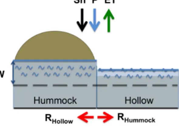
The Hummock–Hollow (HH) model (Cresto Aleina et al., 2015) simulates peatland micro-topographic controls on land–atmosphere fluxes. It is suited to work at 1 m×1 m resolution, which is the typical spatial scale of peatland microtopography. Each grid cell of the HH model represents just one micro-topographic feature, namely a hummock or a hollow. The model simulates a 1 km×1 km peatland and its parameters are tuned with values for a typical peatland in northwestern Russia. In particular, we use the model to simulate the Ust-Pojeg mire in the Komi Republic (61^◦56⁰N, 50^◦13⁰E; 119 m a.s.l.). The site has been extensively studied, and recent efforts described peat characteristics (Pluchon et al., 2014), fluxes of water vapor (Runkle et al., 2012), carbon dioxide (Schneider et al., 2012), and methane (Gažoviˇc et al., 2010), as well as energy and water balance (Runkle et al., 2014) and spatial distribution of dissolved organic carbon (DOC) (Avagyan et al., 2014, 2015). The microtopography is initialized with micro-topographic data collected through surveying with a theodolite. An elevation distribution is derived from the data, and it is possible to randomly assign an elevation at each grid cell (for more information, Cresto Aleina et al., 2015). Depending on the elevation, the grid cell is therefore either a hollow or a hummock (Fig. 1).

For each grid cell (i.e., for each micro-topographic unit) we compute the water balance as

dW_i,j

dt =Sn+P−ET_i,j−R_i,j

s_i,j , (1)

whereWi,j is the water table level in the grid cell at the position(i, j )relative to the surface level, Sn is the snowmelt, P is the precipitation input, ET_i,j is the evapotranspiration, Ri,jis the lateral runoff,si,j is the drainable porosity, andtis time. The time step isδt=1 day. Terms without the indices (i, j )are applied uniformly over the model domain. Water table is computed in respect to the micro-topographic surface, and it is positive above the surface, and negative below it. For a description of the parameterization of Sn and ET_i,j, see Appendix A. This version of the model with the explicit representation of hummocks and hollows is called the Micro- topography configuration.

The HH model can also run in the Single Bucket configuration, where all quantities are averaged over the model domain. Equation (1) becomes therefore

dW

dt =Sn+P−ET−R

s . (2)

The lateral flux is implemented in the same way in the two versions, but in the Microtopography version the water can flow from cell to cell, while in the Single Bucket version the water simply flows out of the system. Cresto Aleina

(3)

Figure 1. Schematics of the HH model showing two grid cells: a hummock and a hollow. The model represents a 1 km×1 km peatland, and works at a 1 m×1 m grid cell. It is therefore able to re- solve the micro-topographical features such as hummocks and hollows. The figure shows two typical grid cells, a hummock and a hollow, and the variables needed for the water table dynamics (Eq. 1 in the text). Each grid cell has an elevation which is randomly assigned from the distribution of elevation data collected in situ. For each grid cell we simulate a dynamical water table, which changes with snowmelt (Sn), precipitation (P), evapotranspiration (ET), and lateral runoff among the different grid cells (Rhummock/hollow). These quantities regulate the change in water table depth (W).

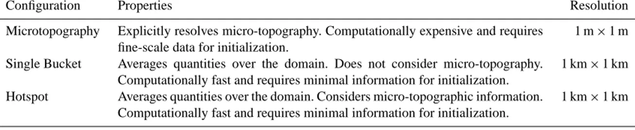
et al. (2015) showed that the Single Bucket configuration, despite being computationally much faster, fails to represent the peatland hydrology, constantly underestimating the water table position in comparison to measurements. This is due to the strong runoff that washes away the water at the beginning of the simulation. Because of the more rugged, hummocky surface represented in the Microtopography version, the runoff is delayed. This behavior better agrees with in situ measurements for water table position (Schneider et al., 2012), whereas the water table position simulated by the HH model in the Single Bucket configuration is too low. Table 1 describes the main differences between the two configurations of the HH model, and the Hotspot parameterization we present in this paper.

2.2 Coupling to a process-based methane emission model

The HH model is coupled to a process-based model for methane emissions, in order to quantify the effect of surface heterogeneities on greenhouse gas fluxes. The model developed by Walter and Heimann (2000) is a quite general model for methane emissions, and it can be applied to peatlands in different environments. It is the same model that is used and coupled with some dynamical global vegetation models (DGVMs) (e.g., Kleinen et al., 2012; Schuldt et al., 2013; Pe- trescu et al., 2008; Zhang et al., 2002). We tuned the model to perform in a typical peatland at the latitude of the Ust- Pojeg mire complex. In the Microtopography configuration,

we computed methane fluxes locally and we averaged over the model domain in order to upscale the local fluxes at the landscape scale. The process-based model for methane emissions provides an output of methane fluxesF_CH^i,j

4as a function of the water table (computed by the HH model), net primary productivity (NPP), and soil temperature (T):

F_CH^i,j

4(t )=f (Wi,j,(t ),NPP(t ), T (t )), (3) whereW_i,j is the water table depth with respect to the surface computed at each position(i, j ). All variables are represented at the daily time step. We force the model with time series of T and NPP taken from CMIP5 experiments performed by the MPI-ESM model. We then considered the model output for the grid cell which corresponds to the Ust- Pojeg mire (see Sect. 2.4). The amount of methane which is emitted by each kind of surface class changes according to the relative position of water table and surface. In the process-based methane emission model developed by Wal- ter and Heimann (2000), the water table is a key variable in methane fluxes, because of the oxidation processes simulated as the water table drops below the surface and as the oxic zone deepens. The HH model in the Microtopography configuration reasonably represents the hydrological interactions among hummocks and hollows and the variability of emissions within the peatland. In the Single Bucket configuration the water table drops quickly below the surface after the snowmelt due to a strong runoff, and thus most of the methane transported from below ground is oxidized. Param- eters for the methane emission model are described in Ap- pendix B.

2.3 The Hotspot parameterization

The HH model has a critical scale of about 0.01 km² at which seasonal results do not change for finer resolutions (Cresto Aleina et al., 2015). Even at this resolution it is un- feasible to include a micro-topography parameterization in the current GCMs.

The general purpose of our Hotspot parameterization is to upscale information from the local to the atmospheric scale.

The HH model identifies different surface types depending on the relative position of the water tableWand the surface:

W > _a ⇒ wet surface,

−b≤W≤a ⇒ saturated surface,

W <−_b ⇒ dry surface.

Here we assume, after Couwenberg and Fritz (2012), the following because of the importance of such thresholds for methane emissions:

a=15 cm, _b=10 cm.

(4)

Table 1. Description of the different configurations of the Hummock–Hollow (HH) model used in the present paper.

Configuration Properties Resolution

Microtopography Explicitly resolves micro-topography. Computationally expensive and requires fine-scale data for initialization.

1 m×1 m Single Bucket Averages quantities over the domain. Does not consider micro-topography.

Computationally fast and requires minimal information for initialization.

1 km×1 km Hotspot Averages quantities over the domain. Considers micro-topographic information.

Computationally fast and requires minimal information for initialization.

1 km×1 km

We assume the saturated surface to be the surface class which dominates the methane emission dynamics, as a water table near to the surface prevents oxidation.

After obtaining the seasonal behavior of the desired surface class, we aim to parameterize of the area covered by the saturated surface class with a fractional numberq, which represents the fraction of the total surface which is saturated at each time step. This information results in a different water table behavior which in turns controls methane emissions.

By knowing the fractionq of saturated surface at each time stept, we implicitly subdivide the domain of the HH model in the Single Bucket versionAin unsaturated surfaceAunsat

and saturated surfaceAsat:

A=(1−q)Aunsat+qAsat. (4)

The position of the water table inA_satstays between−_b≤ W_t^s≤_a, which is given by the definition of the saturated surface, and therefore we assume

W_t^s= −_b+(_a+_b)r, (5)

wherer is a random number between 0 and 1. The position of the water table inAunsat, instead, is the one computed by the HH model in the Single Bucket configuration, i.e.,W in Eq. (2), which responds to precipitation and evapotranspiration. Methane fluxes are calculated as a function of the water table assuming a linear relationship between emitting area and methane fluxes:

FCH₄=(1−q)F_CH^SB

4(W )+qF_CH^sat

4(W_t^s) (6)

where F_CH₄ is the methane flux from the whole domain, F_CH^SB

4 the flux from the HH model in the Single Bucket version, andF_CH^sat

4 the flux from the saturated areaAsat. The saturated area fractionqis defined in Eq. (4). The other forcing variables forFCH₄ stay unchanged, as in Eq. (3).

The specific form ofqas a function of time will be inferred by the analysis of the saturated area dynamics, an output of the HH model in the Microtopography configuration.

2.4 Forcing data

The HH model is forced with prescribed snowmelt, precipitation, and evapotranspiration (Eq. 1). The simulated Sn is a

stochastic input that functions as initialization parameter for the water table. It is parameterized to gain the same magnitude of the observational data (Schneider et al., 2012; Run- kle et al., 2014). Evapotranspiration is simulated according to observations of Runkle et al. (2014) using an empirical parameterization. All parameterizations are described in more detail in the Appendices. In Eq. (1) we assumed Sn andP to be uniform over the whole simulated domain and we did not apply any downscaling further.

We forced the process-based model for methane emissions developed by Walter and Heimann (2000) (Eq. 3) and the water balance (Eq. 1) with prescribed time series of NPP and T, and of precipitationP respectively. The time series are computed from simulations performed for the CMIP5 experiments with the MPI-ESM model at T63 resolution for the grid cell which corresponds to the Ust-Pojeg mire. The potential bias introduced by using NPP of C3 grasses and not the one for mosses (not included in the MPI-ESM model) is negligible as discussed by Cresto Aleina et al. (2015).

We used theP,T, and NPP from the last 30 years of the IPCC historical simulations and forced the model to infer a parameterization of the saturated area (Eqs. 4 and 6) for the past 30-year climatology. To assess the robustness of our parameterization for future simulations we chose three Rep- resentative Concentration Pathways (RCP) scenarios (Taylor et al., 2012), and we therefore considered the identical set of variables from the RCP2.6, RCP4.5, and RCP8.5 experiments from year 2006 to 2099 on daily resolution (Giorgetta et al., 2013).

3 Results and discussion 3.1 Hotspot area dynamics

By averaging the output of the model over 30 years of simulations, from 1976 to 2005 we calculated the average dynamics of the three surface classes: wet, saturated, and dry.

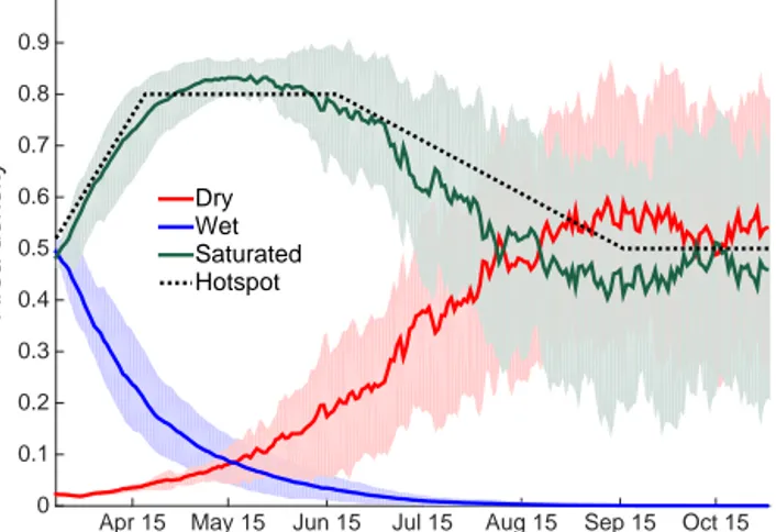
In particular, we are interested in the 30-year average of the saturated areaA_satdynamics (Eq. 4). After snowmelt, most of the simulated peatland surface is either saturated, or wet (Fig. 2). As the simulations continue, surface and subsurface runoff wash water out of the peatland, changing the relative composition of the area densities. More and more cells be-

(5)

Apr 15 May 15 Jun 15 Jul 15 Aug 15 Sep 15 Oct 15

Area density

0 0.1 0.2 0.3 0.4 0.5 0.6 0.7 0.8 0.9 1

Dry Wet Saturated Hotspot

Figure 2. Area densities for dry (red line), wet (blue line), and sat- urated (green line) grid cells. The solid lines represent the different surface class dynamics averaged over 30 years, from 1976 to 2005.

Shaded areas represent standard deviations over the same period of time. The dynamics of the saturated grid cells are mimicked by the empirical Hotspot parameterization (black dotted line), Eq. (7) in the text.

come dry by having a water table lower than 10 cm below the surface. Grid cells belonging to the wet surface class, with a high water table, become saturated and towards the beginning of August virtually no grid cell displays a water table higher than 15 cm above the surface level. At the end of the simulations, almost in all grid cells the water table lies more than 10 cm below the surface level, and the peatland is relatively dry by the end of October.

We used the output of the spatially explicit HH model to describe the dynamics of methane emission hotspots, assuming that the saturated grid cells are the ones where methane emissions are higher. We therefore infer the dynamics of the saturated grid cells from Fig. 2 and obtain the following parameterization for methane emission hotspots:

q(t )=











q_in+qmax−qin

t₁−t₀ (t−t₀) if t≤t₁ qmax if t1< t≤t2

q_max+qmin−qmax

t3−t2

(t−t₂) if t₂< t≤t₃ qmin otherwise

, (7)

wheret is the daily time step of the simulation, and the pa- rameterst_iandq_j are tuned quantities obtained according to the dynamics of saturated grid cells in Fig. 2. Values for the parameterization are described in Table 2. We slightly over- estimate the amount of saturated grid cells in order to take into account the potential methane emission hotspots belonging to the wet surface class.

Table 2. Parameter values for Eq. (7). We infer the values from the dynamics of the grid cells belonging to the saturated surface class as in Fig. 2. Days are computed according to the Julian calendar.

Symbol Meaning Value

t₀ Initial day of simulation 79

t₁ Initial day of maximum saturation 110 t₂ Final day of maximum saturation 170 t₃ Initial day of minimum saturation 260 q_in Initial saturation area density 0.52 qmax Maximum saturation area density 0.8 q_min Minimum saturation area density 0.5

We illustrate the empirical parameterization of the area density computed by Eq. (7) in Fig. 2 (black dotted line).

This parameterization represents the average dynamics of methane emission hotspots for the 30-year period 1976–

2005.

3.2 Methane emissions for 1976–2005

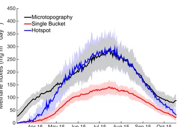
We compared methane emissions from the Ust-Pojeg mire simulated over a 30-year period (1976–2005) in the three versions of the HH model (Table 1). We then averaged the 30 simulations and studied the differences in dynamics among the different HH model versions. The Microtopog- raphy configuration (black line in Fig. 3) produces seasonal fluxes that more than double the cumulative methane fluxes produced by the HH model in the Single Bucket configuration (red line in Fig. 3). In particular towards July and August, when temperatures are higher and methane fluxes larger, the two versions of the HH model diverge in flux esti- mation and the Single Bucket configuration largely underes- timates methane fluxes (Cresto Aleina et al., 2015).

Combining Eqs. (4) and (6), and the empirical parameterization of the hotspot area density q(t ) (Eq. 7), we obtain a new flux dynamics (blue line in Fig. 3). The new parameterized fluxes display similar magnitude and dynamics as the fluxes simulated by the Microtopography configuration, but at a much lower computational cost. The main difference between the emissions from the Single Bucket and Microtopography configurations is the large underestimation in the central part of the summer season, i.e., in July and August. The Hotspot parameterization, by changing the saturated area, improved this feature. The visual improvement is confirmed by the large differences in the seasonally cumulated methane emissions. The differences in cumulative emissions from the three model configurations are summa- rized in Table 3.

The Hotspot parameterization mimics the general magnitude and dynamics of the emissions from the Microtopogra- phy configuration but fails to capture the whole amplitude of methane emissions at the beginning and at the end of the simulations. Such discrepancies might be caused by other vari-

(6)

Table 3. Cumulative emissions from different model configurations. The Single Bucket configuration produces less than the half of the cumulative methane emissions with respect to the model with micro-topography representation. By inserting a simple parameterization of the saturated surface dynamics, we improve significantly the seasonal methane emissions.

Symbol Meaning Value Units

CH^SB₄ Cumulative emissions from the Single Bucket configuration

1.70±0.11×10⁴ mg m⁻² CH^Mic₄ Cumulative emissions from the Microtopography

configuration

3.82±0.30×10⁴ mg m⁻² CH^HS₄ Cumulative emissions from the Single Bucket

configuration with the Hotspot parameterization

3.47±0.25×10⁴ mg m⁻²

Apr 15 May 15 Jun 15 Jul 15 Aug 15 Sep 15 Oct 15 Methane fluxes (mg m-2 day-1 )

0 50 100 150 200 250 300 350 400 450

Microtopography Single Bucket Hotspot

Figure 3. Methane emissions from the HH model coupled with the Walter and Heimann (2000) model. Solid lines are averages over 30 years (1976–2005) and shaded areas represent standard deviations. Emissions are computed using the HH model in the Micro- topography configuration (black line), in the Single Bucket configuration (red line), and in the Single Bucket configuration with the Hotspot parameterization (blue line).

ables which, differently from the water table, remain averaged over the domain. In particular, peat depth is uniform and the model does not have a heterogeneous peat profile as in the Microtopography configuration. This difference may influence the carbon available for methane emissions.

The Hotspot parameterization doubles the cumulative fluxes over the season with respect to the Single Bucket configuration, despite its low computational costs. From an eco- logical perspective, modeling CH₄ fluxes more accurately will improve our estimates of carbon stocks, which may help constrain dynamic vegetation models, bacterial C consump- tion models, and potential feedbacks with the atmosphere.

Also, modeling hydroecological effects of “slower” runoff from a peatland can potentially influence vegetation dynamics of mosses in models including moss dynamics, e.g., Po- rada et al. (2013). The HH model is novel in the physical representation of lateral fluxes of water among hummocks and hollows, but other models representing surface hetero-

geneity controls on water table (e.g., Shi et al., 2015) and methane fluxes (e.g., Bohn et al., 2013) display similar effects. Therefore, and because of the process-based nature of the HH model, we are confident in hypothesizing similar results if a Hotspot-like parameterization was to be applied to other models.

3.3 Future projections with the Hotspot parameterization

The Hotspot parameterization mimics the simulated methane emissions of the Microtopography configuration for the 1976–2005 period for which it has been tuned. We now force the model for the 2006–2099 period with data from the CMIP5 experiments. The HH model does not simulate an increasing trend for methane emissions for the next 100 years, despite the generally higher temperatures (Fig. 4a, c, and e). Even in the RCP8.5 scenario, despite an increase of 4 K in average temperature in year 2099 in respect to the RCP4.5 and the RCP2.6 simulations, we can not find any significant trend. This result is in agreement with the find- ings from the Wetland and Wetland CH₄Inter-comparison of Models Project (WETCHIMP) experiments (Melton et al., 2013), which did not find a large significant trend in methane emissions simulated by the models participating in the inter- comparison project because of increased temperature or of precipitation trends. We use these two variables to force the HH model coupled with the methane emission model.

Such an increase is suggested to reduce stomatal conduc- tance, with the same amount of evapotranspiration, thus increasing waterlogged surface area. In particular, Melton et al.

(2013) did not find a large significant trend in methane emissions simulated by the models participating in the inter- comparison project because of increased temperature or precipitation trends, which are the two variables we use to force the HH model coupled with the methane emission model.

Moreover, future changes in precipitation could potentially affect the water table position and therefore the saturated area fraction which may not correspond to the one described in the Hotspot parameterization. In the RCP simulations, even if precipitation changes in respect to present day and among the scenarios, the differences are not so large

(7)

Figure 4. Performances of the three configurations of the HH model for future projections in different scenarios. Panels (a), (c), and (e) represent seasonally cumulated methane emissions computed by the HH model forced with CMIP5 data for the time period 2006–2099 from the RCP8.5, 4.5, and 2.6 experiments respectively. Panels (b), (d), and (f) represent the seasonal effectiveness of the Hotspot parameterization for future projections, forced with CMIP5 data for the time period 2006–2099 from the RCP8.5, 4.5, and 2.6 experiments respectively. We illustrate the ratio of methane emissions with respect to the Microtopography configuration for the Hotspot parameterization (in blue) and the Single Bucket configuration (in red). We averaged each day of simulation over the 2006–2099 period.

to cause significant effects on methane emissions. In Fig. 4a, c, and e, the outputs of the HH model in the Microtopogra- phy and Single Bucket configurations (i.e., the black and red lines, respectively) have water table explicitly depending on precipitation simulated in the RCP scenarios. The Hotspot parameterization (i.e., blue lines), despite using the saturated area dynamics for the years 1976–2005, is quite close to the methane emissions from the Microtopography configuration.

We then conclude that the potential bias introduced by us-

ing a fixed saturated area dynamics (the one for the period 1976–2005) and not a dynamic one is negligible.

The Single Bucket configuration estimates 42.8–50.8 % of the methane emissions cumulated over the season simulated by the Microtopography configuration with the RCP8.5 scenario forcing. These estimates are very similar with forcing from the RCP4.5 scenario (44.3–50.4 %) and from the RCP2.6 scenario (43.0–50.6 %). If we include the Hotspot parameterization, the simulated annual methane emissions

(8)

range from [2.831–4.321]×10⁴mg m⁻² with the RCP8.5 forcing. This is 83.9–101.5 % of the emissions simulated by the Microtopography configuration. As for the Single Bucket configuration, the numbers are similar for the other forcing scenarios. The simulated emissions range from [2.771–

4.056]×10⁴mg m⁻² (88.4–100.1 % of the emissions in the Microtopography configuration) for the RCP4.5 scenario, and [2.648–4.102]×10⁴mg m⁻²(87.7–104.3 % of the emissions in the Microtopography configuration) for the RCP2.6 scenario. The amplitude and timing of year-to-year variability of cumulative methane emissions with the Hotspot parameterization are also comparable to the ones simulated by the Microtopography configuration in all simulated scenarios.

These results increase the applicability of the Hotspot parameterization. Despite being tuned for the 1976–2005 climatology, it works for the next century of simulations under very different forcing scenarios. This is due to the large differences in hydrological representations between the Micro- topography and Single Bucket configurations. Such differences are almost totally overcome with the use of the Hotspot parameterization. These improvements make the parameterization applicable also for future time slices, despite the differences in temperature, precipitation, and NPP forcing between the time period used for the parameterization tuning and the scenario projections.

We also tested the effectiveness of the Hotspot parameterization over the seasonal cycle. We averaged for each simulated day the methane emissions over the 2005–2099 period for all model configurations and for all scenarios. We then di- vided the daily emissions from the Single Bucket configuration and from the Hotspot parameterization by the emissions from the Microtopography configuration to investigate the impact of the new parameterization on the seasonal cycle. In all simulated scenarios, the Hotspot parameterization works very well during the mid-season. From mid-May till the beginning of October, when methane emissions are higher, the ratio between the Hotspot parameterization and the Micro- topography parameterization is near one (Fig. 4b, d, and f).

The ratio between emissions from the Single Bucket configuration and the Microtopography configuration reaches its maximum only towards the end of the simulations, therefore missing the larger methane emissions peaks in June, July, and August.

4 Summary and conclusions

We developed a new parameterization to bridge the scaling gap between a process-based, small-scale hydrological model for peatlands, and a mean field approximation, analogous to a large-scale parameterization in a DGVM.

The Hotspot parameterization uses the output of the HH (Hummock–Hollow) model (Cresto Aleina et al., 2015), which simulates a 1 km×1 km peatland. The HH model can work in both configurations, a spatially explicit one work-

ing at 1 m×1 m scale, simulating explicitly hummocks and hollows (the Microtopography configuration), and a mean field approximation of it, where all quantities are averaged over the domain (the Single Bucket configuration). If coupled to a process-based methane emission model (Walter and Heimann, 2000) the Microtopography configuration simulates more realistic methane fluxes because of the better representation of hydrology due to the explicit description of processes at 1 m scale, but at a much higher computational cost. We assumed that the lack of representation of saturated areas in the Single Bucket configuration, which are methane emission hotspots, diminishes the cumulative emissions over the season by half.

We inferred a parameterization of this hotspot area for emissions for the period 1976–2005, which are the last 30 years of the historical simulations from the CMIP5 experiments. We analyzed the spatial pattern of the HH model output in the Microtopography configuration averaged over the 30 simulated years. We introduced this information in the Single Bucket configuration, modifying the hydrology of the mean field approximation, obtaining the Hotspot parameterization. This novel approach that takes into account the information from the spatially explicit simulations bridges the gaps between the simulated methane emissions. The Hotspot parameterization, due to its higher modified water table, is able to mimic the general magnitude and dynamics of the emissions from the model with micro-topography representation.

By forcing the model with time series of temperature, NPP, and precipitation for the next century from CMIP5 experiments in the RCP8.5, RCP4.5, and RCP2.6 scenarios, we as- sessed the robustness of the Hotspot parameterization under forcing for which it was not originally calibrated. The parameterization holds for years 2006–2099 for all three scenarios.

Overall, the ratio between the seasonally cumulated emissions from the HH model in the Microtopography configuration and the ones simulated by the Hotspot parameterization ranges between 0.84 and 1.04. This is a substantial improvement in comparison to the methane emissions simulated by the Single Bucket configuration, which only produces between 43 and 51 % of the seasonally cumulated methane emissions. The Hotspot parameterization at almost no computational cost therefore qualitatively changes and improves the simulated system response for methane emissions.

We only applied this method to the HH model simulating a single peatland in western Russia. This method, though, uses the information of a mechanistic, spatially explicit model and it is a significant first step towards a full parameterization of the micro-topographic impacts on complex ecosystems at the DGVM scale. In order to develop such a parameterization we would need a comprehensive and statistical analysis on the response of the mechanistic local-scale model to different climatic forcing: we would need HH-like models working at the micro-topographic scale applied at different peatlands in other climatic zones. Another limitation of the

(9)

applicability of this study is its dependency on the avail- ability of data to calibrate the original HH model in its Mi- crotopography configuration, as accurate measurements of peatland micro-relief are needed to initialize surface height.

While it is not realistic to have theodolite micro-topographic measurements globally, other methods and products could help provide similar information. Aerial photographs provide some information on micro-topography, but generally at an overly coarse scale. Statistical downscaling methods as the ones used, e.g., by Muster et al. (2012) and Stoy and Quaife (2015) are therefore needed to infer information on surface heterogeneities, but they are not necessarily useful

in identifying micro-topography distribution. Airborne measurements could aid in giving qualitative and stochastic information also on structural peatland patterns, such as the ones described by Couwenberg and Joosten (2005). This information could be used by the HH model to generate nonran- dom configurations, potentially investigating the influence of structured patterns on hydrology and methane emissions.

Introducing the analysis of spatial patterns produced by different mechanistic models in multiple ecosystems is a powerful method to infer landscape-scale dynamics and characteristics of patterns.

(10)

Appendix A: Climatology parameterization

Cresto Aleina et al. (2015) did not consider the snowmelt Sn, since they started the simulations later on and, therefore, initialized the water table to match the observations at the end of April. Sn represents the water input at the beginning of the warm season. The cold season is not represented in the model, because we assume that snow covers the area (almost) uniformly. We compute the snowmelt as a random number varying between 200 and 300 mm. We used this range for Sn in order to obtain an initial water table level on the same order of magnitude of the one observed by Schneider et al.

(2012) and Runkle et al. (2014).

Evapotranspiration is dependent on the soil dryness and patchiness. We refer to former studies (Nichols and Brown, 1980), which extensively analyzed the evaporation rate from Sphagnum moss surfaces. The evapotranspiration rate de- pends on the day of the season, the surface wetness, and on the micro-topographic features.

ET_i,j=









 ET^max_i,j

fr(Wi,j)sin((t−4t₀)π 6t0

) if 180< t <300 ET^max_i,j

fr(Wi,j) otherwise

, (A1)

wheretis the daily time step in days of Julian calendar,t0= 30 days is a time constant, and ET^max_i,j is a function of the micro-topographic features for the cell at the positioni, j:

ET^max_i,j =

6 mm d⁻¹ if hummock

3 mm d⁻¹ if hollow. (A2)

fr(W_i,j) takes into account the fact that evaporation takes place at a higher rate if the water table is above the surface:

fr(Wi,j)=

1 ifWi,j above the surface level

2 ifWi,j below the surface level. (A3) We use this very simple parameterization of the evapotranspiration rate in order to study the general response of the model to random climatic conditions and to produce quantities in the order of the ones measured by Runkle et al. (2014).

Appendix B: Parameters for the methane emission model

We tuned the parameters used in the process-based model for methane emissions (Walter and Heimann, 2000) in order to apply the model at the latitude of the Ust-Pojeg Mire complex, in the Komi Republic, Russia (61^◦56⁰N, 50^◦13⁰E;

119 m a.s.l.). Walter and Heimann (2000) used a tuning parameter for the model,R0, which we fix at 0.30. Another parameter needed to couple with the methane emission model is the soil depth, which we fixed at 150 cm following in situ observation (Pluchon et al., 2014).

(11)

Acknowledgements. F. Cresto Aleina, B. R. K. Runkle, T. Brücher, and V. Brovkin have been supported by the Cluster of Excellence

“CliSAP” (EXC177) of the University of Hamburg, as funded by the German Research Foundation (DFG). The authors would like to acknowledge Lars Kutzbach for the help and fruitful discussions which led to significant model improvements. The authors also thank the three anonymous reviewers who with their comments greatly helped in increasing the clarity and the quality of the paper.

The article processing charges for this open-access publication were covered by the Max Planck Society.

Edited by: T. Kato

References

Acharya, S., Kaplan, D. A., Casey, S., Cohen, M. J., and Jawitz, J. W.: Coupled local facilitation and global hydrologic inhi- bition drive landscape geometry in a patterned peatland, Hy- drol. Earth Syst. Sci., 19, 2133–2144, doi:10.5194/hess-19-2133- 2015, 2015.

Avagyan, A., Runkle, B., Hartmann, J., and Kutzbach, L.: Spatial Variations in Pore-Water Biogeochemistry Greatly Exceed Tem- poral Changes During Baseflow Conditions in a Boreal River Valley Mire Complex, Northwest Russia, Wetlands, 34, 1171–

1182, doi:10.1007/s13157-014-0576-4, 2014.

Avagyan, A., Runkle, B. R. K., Hennings, N., Haupt, H., Virta- nen, T., and Kutzbach, L.: Dissolved organic matter dynamics during the spring snowmelt at a boreal river valley mire complex in Northwest Russia, Hydrol. Process., online first, doi:

10.1002/hyp.10710, 2015.

Baird, A. J., Belyea, L. R., and Morris, P. J.: Carbon Cy- cling in Northern Peatlands, Geophysical Monograph Series, vol. 184, American Geophysical Union, Washington, D. C., USA, doi:10.1029/GM184, 2009.

Baudena, M., von Hardenberg, J., and Provenzale, A.: Vegetation patterns and soil-atmosphere water fluxes in drylands, Adv. Wa- ter Resour., 53, 131–138, doi:10.1016/j.advwatres.2012.10.013, 2013.

Baudena, M., Sánchez, A., Georg, C.-P., Ruiz-Benito, P., Ro- driguez, M. A., Zavala, M. A., and Rietkerk, M.: Revealing patterns of local species richness along environmental gradi- ents with a novel network tool, Scientific Reports, 5, 11561, doi:10.1038/srep11561, 2015.

Bohn, T. J., Podest, E., Schroeder, R., Pinto, N., McDonald, K.

C., Glagolev, M., Filippov, I., Maksyutov, S., Heimann, M., Chen, X., and Lettenmaier, D. P.: Modeling the large-scale effects of surface moisture heterogeneity on wetland carbon fluxes in the West Siberian Lowland, Biogeosciences, 10, 6559–6576, doi:10.5194/bg-10-6559-2013, 2013.

Couwenberg, J. and Fritz, C.: Towards developing IPCC methane

“emission factors” for peatlands (organic soils), Mires and Peat, 10, 1–17, 2012.

Couwenberg, J. and Joosten, H.: Self-organization in raised bog pat- terning: the origin of microtope zonation and mesotope diversity, J. Ecol., 93, 1238–1248, doi:10.1111/j.1365-2745.2005.01035.x, 2005.

Cresto Aleina, F., Brovkin, V., Muster, S., Boike, J., Kutzbach, L., Sachs, T., and Zuyev, S.: A stochastic model for the polygonal tundra based on Poisson–Voronoi diagrams, Earth Syst. Dynam., 4, 187–198, doi:10.5194/esd-4-187-2013, 2013.

Cresto Aleina, F., Runkle, B. R. K., Kleinen, T., Kutzbach, L., Schneider, J., and Brovkin, V.: Modeling micro-topographic controls on boreal peatland hydrology and methane fluxes, Biogeo- sciences, 12, 5689–5704, doi:10.5194/bg-12-5689-2015, 2015.

Dekker, S. and Rietkerk, M.: Coupling microscale vegetation- soil water and macroscale vegetation-precipitation feedbacks in semiarid ecosystems, Glob. Change Biol., 13, 671–678, doi:10.1111/j.1365-2486.2007.01327.x, 2007.

Gažoviˇc, M., Kutzbach, L., Schreiber, P., Wille, C., and Wilmk- ing, M.: Diurnal dynamics of CH₄ from a boreal peatland during snowmelt, Tellus B, 62, 133–139, doi:10.1111/j.1600- 0889.2010.00455.x, 2010.

Giorgetta, M. A., Jungclaus, J., Reick, C. H., Legutke, S., Bader, J., Böttinger, M., Brovkin, V., Crueger, T., Esch, M., Fieg, K., Glushak, K., Gayler, V., Haak, H., Hollweg, H.-D., Ilyina, T., Kinne, S., Kornblueh, L., Matei, D., Mauritsen, T., Mikolajew- icz, U., Mueller, W., Notz, D., Pithan, F., Raddatz, T., Rast, S., Redler, R., Roeckner, E., Schmidt, H., Schnur, R., Segschnei- der, J., Six, K. D., Stockhause, M., Timmreck, C., Wegner, J., Widmann, H., Wieners, K.-H., Claussen, M., Marotzke, J., and Stevens, B.: Climate and carbon cycle changes from 1850 to 2100 in MPI-ESM simulations for the Coupled Model Intercom- parison Project phase 5, J. Adv. Model. Earth Sys., 5, 572–597, doi:10.1002/jame.20038, 2013.

Gong, J., Wang, K., Kellomäki, S., Zhang, C., Martikainen, P. J., and Shurpali, N.: Modeling water table changes in boreal peatlands of Finland under changing climate conditions, Ecol. Model., 244, 65–78, doi:10.1016/j.ecolmodel.2012.06.031, 2012.

Gong, J., Kellomäki, S., Wang, K., Zhang, C., Shurpali, N., and Martikainen, P. J.: Modeling CO₂and CH₄flux changes in pris- tine peatlands of Finland under changing climate conditions, Ecol. Model., 263, 64–80, doi:10.1016/j.ecolmodel.2013.04.018, 2013.

Hugelius, G., Tarnocai, C., Broll, G., Canadell, J. G., Kuhry, P., and Swanson, D. K.: The Northern Circumpolar Soil Carbon Database: spatially distributed datasets of soil coverage and soil carbon storage in the northern permafrost regions, Earth Syst.

Sci. Data, 5, 3–13, doi:10.5194/essd-5-3-2013, 2013.

Janssen, R. H. H., Meinders, M. B. J., van Nes, E. H., and Schef- fer, M.: Microscale vegetation-soil feedback boosts hysteresis in a regional vegetation–climate system, Glob. Change Biol., 14, 1104–1112, doi:10.1111/j.1365-2486.2008.01540.x, 2008.

Kleinen, T., Brovkin, V., and Schuldt, R. J.: A dynamic model of wetland extent and peat accumulation: results for the Holocene, Biogeosciences, 9, 235–248, doi:10.5194/bg-9-235-2012, 2012.

Melton, J. R., Wania, R., Hodson, E. L., Poulter, B., Ringeval, B., Spahni, R., Bohn, T., Avis, C. A., Beerling, D. J., Chen, G., Eliseev, A. V., Denisov, S. N., Hopcroft, P. O., Lettenmaier, D.

P., Riley, W. J., Singarayer, J. S., Subin, Z. M., Tian, H., Zürcher, S., Brovkin, V., van Bodegom, P. M., Kleinen, T., Yu, Z. C., and Kaplan, J. O.: Present state of global wetland extent and wetland methane modelling: conclusions from a model inter- comparison project (WETCHIMP), Biogeosciences, 10, 753–

788, doi:10.5194/bg-10-753-2013, 2013.

(12)

Muster, S., Langer, M., Heim, B., Westermann, S., and Boike, J.: Subpixel heterogeneity of ice-wedge polygonal tundra:

a multi-scale analysis of land cover and evapotranspiration in the Lena River Delta, Siberia, Tellus B, 1, 1–19, doi:10.3402/tellusb.v64i0.17301, 2012.

Nichols, D. S. and Brown, J. M.: Evaporation from a sphagnum moss surface, J. Hydrol., 48, 289–302, doi:10.1016/0022- 1694(80)90121-3, 1980.

Nungesser, M. K.: Modelling microtopography in boreal peatlands: hummocks and hollows, Ecol. Model., 165, 175–207, doi:10.1016/S0304-3800(03)00067-X, 2003.

Peng, J., Loew, A., Zhang, S., and Wang, J.: Spatial downscaling of satellite soil moisture data using a temperature vegetation dryness index, IEEE T. Geosci. Remote, 54, 558–566, doi:10.1109/TGRS.2015.2462074, 2016.

Petrescu, A. M. R., van Huissteden, J., Jackowicz-Korczynski, M., Yurova, A., Christensen, T. R., Crill, P. M., Bäckstrand, K., and Maximov, T. C.: Modelling CH₄ emissions from arctic wetlands: effects of hydrological parameterization, Biogeosciences, 5, 111–121, doi:10.5194/bg-5-111-2008, 2008.

Pluchon, N., Hugelius, G., Kuusinen, N., Kuhry, P., Pluchon, N., Hugelius, G., and Kuusinen, N.: The Holocene storage in two boreal peatlands of Northeast European Russia, The Holocene, 24, 1126–1136, doi:10.1177/0959683614523803, 2014.

Porada, P., Weber, B., Elbert, W., Pöschl, U., and Kleidon, A.:

Estimating global carbon uptake by lichens and bryophytes with a process-based model, Biogeosciences, 10, 6989–7033, doi:10.5194/bg-10-6989-2013, 2013.

Raddatz, T., Reick, C., Knorr, W., Kattge, J., Roeckner, E., Schnur, R., Schnitzler, K.-G., Wetzel, P., and Jungclaus, J.: Will the trop- ical land biosphere dominate the climate–carbon cycle feedback during the twenty-first century?, Clim. Dynam., 29, 565–574, doi:10.1007/s00382-007-0247-8, 2007.

Reick, C., Raddatz, T., Brovkin, V., and Gayler, V.: Representation of natural and anthropogenic land cover change in MPI-ESM, J.

Adv. Model. Earth Sys., 5, 459–482, 2013.

Rietkerk, M. and van de Koppel, J.: Regular pattern formation in real ecosystems, Trends Ecol. Evol. (Personal edition), 23, 169–

175, doi:10.1016/j.tree.2007.10.013, 2008.

Runkle, B., Wille, C., Gažoviˇc, M., Wilmking, M., and Kutzbach, L.: The surface energy balance and its drivers in a boreal peatland fen of northwestern Russia, J. Hydrol., 511, 359–373, doi:10.1016/j.jhydrol.2014.01.056, 2014.

Runkle, B. R. K., Wille, C., Gažoviˇc, M., and Kutzbach, L.: At- tenuation Correction Procedures for Water Vapour Fluxes from Closed-Path Eddy-Covariance Systems, Bound.-Lay. Meteorol., 142, 401–423, doi:10.1007/s10546-011-9689-y, 2012.

Sachs, T., Giebels, M., Boike, J., and Kutzbach, L.: Environmen- tal controls on CH₄emission from polygonal tundra on the mi- crosite scale in the Lena river delta, Siberia, Glob. Change Biol., 16, 3096–3110, doi:10.1111/j.1365-2486.2010.02232.x, 2010.

Schmidt, M. W. I., Torn, M. S., Abiven, S., Dittmar, T., Guggen- berger, G., Janssens, I. A., Kleber, M., Kogel-Knabner, I., Lehmann, J., Manning, D. A. C., Nannipieri, P., Rasse, D. P., Weiner, S., and Trumbore, S. E.: Persistence of soil organic matter as an ecosystem property., Nature, 478, 49–56, doi:10.1038/nature10386, 2011.

Schneider, J., Kutzbach, L., and Wilmking, M.: Carbon dioxide ex- change fluxes of a boreal peatland over a complete growing season, Komi Republic, NW Russia, Biogeochemistry, 111, 485–

513, doi:10.1007/s10533-011-9684-x, 2012.

Schuldt, R. J., Brovkin, V., Kleinen, T., and Winderlich, J.: Mod- elling Holocene carbon accumulation and methane emissions of boreal wetlands – an Earth system model approach, Biogeo- sciences, 10, 1659–1674, doi:10.5194/bg-10-1659-2013, 2013.

Shi, X., Thornton, P. E., Ricciuto, D. M., Hanson, P. J., Mao, J., Sebestyen, S. D., Griffiths, N. A., and Bisht, G.: Represent- ing northern peatland microtopography and hydrology within the Community Land Model, Biogeosciences, 12, 6463–6477, doi:10.5194/bg-12-6463-2015, 2015.

Shur, Y. L. and Jorgenson, M. T.: Patterns of permafrost formation and degradation in relation to climate and ecosystems, Per- mafrost Periglac., 18, 7–19, doi:10.1002/ppp.582, 2007.

Stoy, P. C. and Quaife, T.: Probabilistic Downscaling of Re- mote Sensing Data with Applications for Multi-Scale Bio- geochemical Flux Modeling, PLoS ONE, 10, e0128935, doi:10.1371/journal.pone.0128935, 2015.

Tarnocai, C., Canadell, J. G., Schuur, E. A. G., Kuhry, P., Mazhi- tova, G., and Zimov, S.: Soil organic carbon pools in the northern circumpolar permafrost region, Global Biogeochem. Cy., 23, GB2023, doi:10.1029/2008GB003327, 2009.

Taylor, K. E., Stouffer, R., and Meehl, G. A.: An overview of cmip5 and the experiment design, B. Am. Meteorol. Soc., 93, 485–498, doi:10.1175/BAMS-D-11-00094.1, 2012.

Van der Ploeg, M. J., Appels, W. M., Cirkel, D. G., Oost- erwoud, M. R., Witte, J.-P., and van der Zee, S.: Microto- pography as a Driving Mechanism for Ecohydrological Pro- cesses in Shallow Groundwater Systems, Vadose Zone J., 11, doi:10.2136/vzj2011.0098, 2012.

Walter, B. P. and Heimann, M.: A process-based, climate-sensitive model to derive methane emissions from natural wetlands: Ap- plication to five wetland sites, sensitivity to model parameters, and climate, Global Biogeochem. Cy., 14, 745–765, 2000.

Zhang, Y., Li, C., Trettin, C. C., Li, H., and Sun, G.: An integrated model of soil, hydrology, and vegetation for carbon dynamics in wetland ecosystems, Global Biogeochem. Cy., 16, 1061, doi:10.1029/2001GB001838, 2002.