Atmospheric Thermal Properties of Venus and Mars -

(1)

Atmospheric Thermal Properties of Venus and Mars

-

Investigation of CO

2

Absorption Lines using Ground-Based Mid-Infrared Heterodyne Spectroscopy

Inaugural - Dissertation zur

Erlangung des Doktorgrades

der Mathematisch-Naturwissenschaftlichen Fakult¨ at der Universit¨ at zu K¨ oln

vorgelegt von

Tobias Stangier

aus K¨ oln

(2)

Tag der m¨ undlichen Pr¨ ufung: 13. Oktober 2014

(3)

List of Figures

1.1 Atmospheric structure of Venus and Mars . . . . 8

1.2 Typical IR heterodyne spectrum from Venus and Mars . . . . 9

2.1 Schematic view on the heterodyne principle . . . . 12

2.2 From a homodyne to a heterodyne spectrum . . . . 14

2.3 Molecular ro-vibrational spectrum of CO

₂

. . . . 18

2.4 Composition of a inhomogeneously broadened line . . . . 20

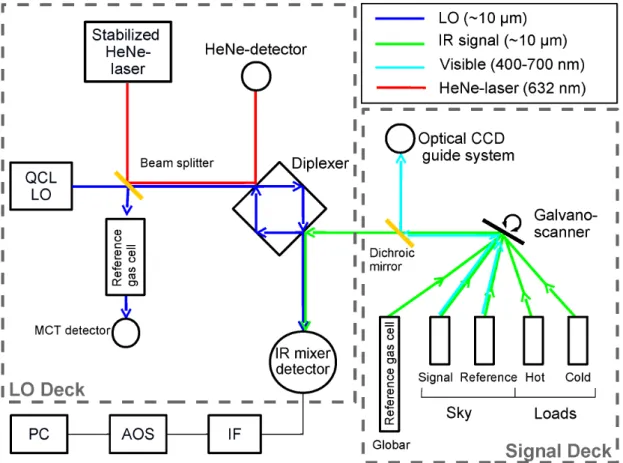
2.5 Schematic view on the beam path in This . . . . 22

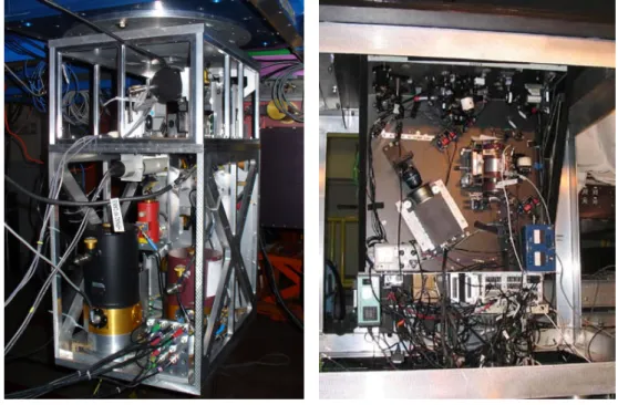
2.6 Photos of This and Hipwac . . . . 23

2.7 Energy diagram of a QCL . . . . 24

2.8 Schematic view on the beam path in Hipwac . . . . 26

2.9 Spectral stability of This . . . . 30

3.1 Illustrations of the geometrical conditions for the model . . . . 35

3.2 Schematic view on the Ifr . . . . 39

3.3 Examples of oscillating pT-profiles . . . . 42

3.4 Synthetic spectra for Venus nightside atmosphere . . . . 43

3.5 Scale factor vs. background radiation . . . . 44

3.6 Fit guess for synthetic spectra . . . . 46

3.7 Retrieved pT-profiles from synthetic data . . . . 47

3.8 Normalized altitude weighting functions . . . . 49

3.9 Comparison between input and output model . . . . 50

4.1 Images of Venus . . . . 52

4.2 Venus Express spacecraft and orbit . . . . 56

4.3 Comparison of probing altitudes . . . . 57

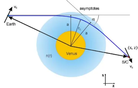
4.4 Ray bending for VeRa in Venus’ atmosphere . . . . 58

4.5 Temperature profile from VeRa . . . . 59

4.6 Virtis temperature map of the southern hemisphere . . . . 61

4.7 Temperature profile from Soir . . . . 62

4.8 pT- and VMR-profile from sub-mm observations at the JCMT . . . 64

V

(8)

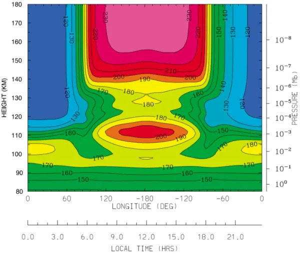
4.10 Temperature profile from Vtgcm . . . . 68

4.11 Temperature profile from Lmd - Gcm . . . . 70

4.12 Observing geometry of Venus for campaign A . . . . 72

4.13 Observing geometry of Venus for campaign B . . . . 73

4.14 Variation of Venusian nightside spectra . . . . 75

4.15 Spectrum from campaign A at EQLT20 . . . . 77

4.16 Spectrum from campaign A at EQLT22 . . . . 78

4.17 Spectrum from campaign B at 67NLT0 . . . . 79

4.18 Spectrum from campaign B at 33SDL . . . . 80

4.19 Temperature profile at EQLT20 . . . . 84

4.20 Temperature profile at EQLT22 . . . . 85

4.21 Temperature profile at 67NLT0 . . . . 87

4.22 Temperature profile at 33SDL . . . . 88

4.23 Temperature profile at 33SDL . . . . 89

4.24 pT-VeRa-profiles from Vex orbit 2218–2223 . . . . 91

4.25 33SDL compared to VeRa coordination . . . . 94

4.26 Rescaled pT-VeRa-profiles from Vex orbit 2220–2222 . . . . 95

4.27 33SDL compared to rescaled VeRa coordination . . . . 96

4.28 EQLT20 and EQLT22 compared to VeRa . . . . 98

4.29 67NLT0 compared to VeRa . . . . 99

4.30 EQLT20 and EQLT22 compared to Virtis . . . 101

4.31 67NLT0 and 33SDL compared to Virtis . . . 102

4.32 EQLT20 and EQLT22 compared to Soir . . . 103

4.33 67NLT0 compared to Soir . . . 104

4.34 33SDL compared to Soir . . . 105

4.35 Observing geometry during sub-millimeter observations . . . 107

4.36 pT-profiles from sub-millimeter observations . . . 108

4.37 EQLT20 and EQLT22 compared to sub-mm profiles . . . 109

4.38 67NLT0 and 33SDL compared to sub-mm profiles . . . 110

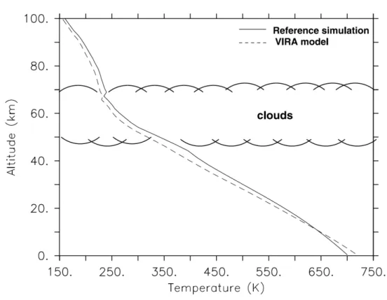
4.39 Vira pT-profiles for all nightside latitudes . . . 112

4.40 EQLT20 and EQLT22 compared to Vira . . . 113

4.41 EQLT20 and EQLT22 compared to Vira . . . 114

4.42 Comparison of all pT-profiles . . . 116

5.1 Images of Mars . . . 120

5.2 Kinetic temperatures from IR heterodyne non-LTE . . . 122

5.3 Synthetic spectra and pT-profiles for Mars - 1 . . . 125

5.4 Synthetic spectra and pT-profiles for Mars - 2 . . . 126

5.5 Observing geometry of Mars for campaign C . . . 128

5.6 Spectrum from campaign C at 45NLT10 . . . 131

5.7 Temperature profile at 45NLT10 . . . 132

VI

(9)

LIST OF FIGURES

6.1 Temperature profile in Titan’s Atmosphere . . . 137

6.2 Ethan emission line from Titan . . . 138

6.3 Ozone absorption feature and stratospheric dynamics . . . 140

C.1 Spectrum from campaign A at EQLT20 in high resolution . . . 161

C.2 Spectrum from campaign A at EQLT22 in high resolution . . . 162

C.3 Spectrum from campaign B at 67NLT0 in high resolution . . . 163

C.4 Spectrum from campaign B at 33SDL in high resolution . . . 164

D.5 Spectrum from campaign C at 45NLT10 in high resolution . . . 165

VII

(10)

(11)

List of Tables

2.1 Applied QCL-LO in This . . . . 24

2.2 Specifications for This and Hipwac . . . . 28

4.1 Orbital parameters of Venus and Earth . . . . 53

4.2 Atmospheric parameters of Venus and Earth . . . . 55

4.3 Overview of the observing campaigns A and B. . . . . 71

4.4 Overview of the observing geometry in 2012 . . . . 74

4.5 Overview of spectral properties . . . . 81

4.6 pT-Profiles from IR-heterodyne observations on Venus . . . . 82

4.7 Overview of thermal profile properties . . . . 83

4.8 Observing geometry of VeRa during coordinated campaign . . . . . 90

4.9 Geometrical parameters for sub-mm observations on Venus nightside 107 5.1 Orbital parameters of Mars and Earth . . . 121

5.2 Atmospheric parameters of Mars and Earth . . . 121

5.3 Overview of the observing campaign C . . . 129

5.4 Overview of the observing geometry in 2010 . . . 129

5.5 pT-Profile from IR-heterodyne observation on Mars . . . 130

C.1 Details of the observing geometry in 2012 . . . 166

IX

(12)

(13)

Kurzzusammenfassung

Die thermischen Eigenschaften verschiedener atmosph¨ arischer H¨ ohenlagen erd¨ ahn- licher Planeten k¨ onnen aus druckverbreiterten Molek¨ ul¨ uberg¨ angen ermittelt wer- den. Mittels bodengebundener Heterodynspektroskopie werden einzelne solcher druckverbreiterten CO

₂

-Absorptionslinien bei 10 µm Wellenl¨ ange auf der Nacht- seite des Planeten Venus beobachtet. Außerdem wird ein Spektrum von der Tagseite des Mars untersucht, welches ebenfalls eine verbreiterte Absorptionslinie aufweist. Infrarot-Heterodynspektroskopie ist auf die atmosph¨ arischen Schichten sensitiv, in denen die Absorption stattfindet. Auf der Venus entspricht dies H¨ ohen- lagen in der Mesosph¨ are zwischen ∼ 60–95 km. Auf dem Mars findet die Absorp- tion in der Troposph¨ are zwischen der Oberfl¨ ache und einer H¨ ohe von ∼ 35 km statt.

Die atmosph¨ arischen Parameter werden mit einer auf dem Levenberg-Marquard- Optimierungsalgorithmus basierenden R¨ uckw¨ artsroutine erlangt. Diese vergle- icht iterativ die Beobachtungsdaten mit Planetenspektren, welche mit Hilfe eines Strahlungstransportmodells unter Ber¨ ucksichtigung des irdischen spektralen Trans- missionsgrads in der obersten planetaren Atmosph¨ are errechnet wurden. Ein de- taillierter proof of concept wird durchgef¨ uhrt, um den Einfluss der H¨ ohenaufl¨ osung zu untersuchen und um die Verl¨ asslichkeit der neu entwickelten Routine zu be- st¨ atigen.

W¨ ahrend zweier Beobachtungskampagnen, die im M¨ arz und im Mai 2012 stattge- funden haben, sind vier verschiedene Positionen auf der Nachtseite der Venus beobachtet worden. In dieser Arbeit werden erstmalig die an den jeweiligen Posi- tionen erlangten Temperaturprofile pr¨ asentiert. Die H¨ ohenaufl¨ osung der erhal- tenen Profile betr¨ agt ∼ 4.5 km. Die so erhaltenen Profile werden mit bereits bekannten Temperaturmessungen anderer luft- und bodengebundener Beobach- tungsmethoden, sowie mit der Venus International Reference Atmosphere ver- glichen. Die gemessenen Temperaturen stimmen gut mit den gefundenen Daten anderer Beobachtungstechniken ¨ uberein. Ein besonderes Augenmerk liegt auf dem Vergleich der an einer speziellen Beobachtungsposition erhaltenen Temperaturen

1

(14)

mit denen, die zeitgleich w¨ ahrend einer koordinierten Messreihe im Mai 2012 mit dem Venus Express Radio Science Experiment gemessen worden sind. Zus¨ atzlich zu existierenden Beobachtungstechniken k¨ onnen nunmehr heterodyne Infrarot- Beobachtungen von hochaufgel¨ osten Spektrallinien Temperaturmessungen von der Nachtseite der Venus liefern.

Die Untersuchung von verbreiterten CO

2

-Absorptionslinien auf der Tagseite vom

Mars wurde an einem Spektrum durchgef¨ uhrt, das w¨ ahrend einer Beobachtungs-

kampagne im Jahr 2010 aufgenommen wurde. Die vorl¨ aufigen Ergebnisse des

erhaltenen Temperaturprofils werden hier nun pr¨ asentiert. Das erhaltene Pro-

fil wird mit einer Vorhersage aus der Mars Climate Database verglichen, zu der

eine zufriedenstellende ¨ Ubereinstimmung gefunden werden kann. Ein weiterer,

ausf¨ uhrlicher proof of concept wird durchgef¨ uhrt, um die besonderen atmosph¨ ari-

schen Bedingungen f¨ ur den Mars zu ber¨ ucksichigen und um den Beitrag der, da

durch Sonneneinstrahlung hervorgerufen nur auf der Tagseite pr¨ asenten, nicht-

thermischen Emissionslinien auf die Auswerteroutine zu untersuchen. Die Auswer-

tung von atmosph¨ arischen Temperaturen auf der Tagseite des Mars unterliegt

zus¨ atzlichen Einschr¨ ankungen, die in erster Linie von der d¨ unnen Atmosph¨ are

und der vielf¨ altigen Topografie der Marsoberfl¨ ache herr¨ uhren.

(15)

Abstract

Atmospheric thermal properties of different altitude layers of terrestrial planets can be deduced from pressure-broadened molecular transition features. Ground-based heterodyne spectroscopy is used to observe the nightside of Venus by probing single pressure-broadened CO

₂

absorption lines at around 10 µm. In addition, a dayside spectrum of Mars, also containing a pressure-broadened absorption feature was investigated. Infrared heterodyne spectroscopy is sensitive to those atmospheric layers, which can be identified as the absorption line formation region. These layers correspond to an altitude range in the Venusian mesosphere between ∼ 60 and ∼ 95 km. On Mars, the line formation region is located in the troposphere between the surface and an altitude of ∼ 35 km.

Retrieval of atmospheric parameters is based on a Levenberg-Marquard χ

²

op- timization that iteratively compares observed data to telluric transmittance cor- rected planetary top-of-atmosphere spectra calculated using a radiative transfer algorithm. A sophisticated proof of concept is performed to investigate the in- fluence of the altitude resolution and to demonstrate the reliability of the newly developed retrieval technique.

During two observing campaigns in March and May 2012, four different locations on the Venusian nightside hemisphere were investigated. In this thesis, the re- trieval of vertical temperature profiles in the nightside atmosphere of Venus using mid-infrared heterodyne spectroscopy is reported for the first time. The retrieval can be deduced with an altitude resolution of ∼ 4.5 km. The retrieved profiles are compared to existing space- and ground-based observations as well as to the Venus International Reference Atmosphere. The temperatures found are in good agreement to other retrieval techniques. Emphasis is given to the comparison of the temperatures from one specific location to thermal profiles simultaneously ob- tained with the Venus Express Radio Science Experiment during a coordinated observing campaign in May 2012. Sub-Doppler resolution infrared heterodyne ob- servations can now provide temperature measurements on the dark side of Venus that complement those techniques.

3

(16)

Analysis of a broad CO

₂

absorption feature obtained at the Martian dayside dur-

ing an observing campaign in 2010 is performed and a preliminary temperature

profile is retrieved. This profile is compared to predictions from the Mars Cli-

mate Database and found to be in satisfactory agreement. A further detailed poof

of concept is provided, addressing the specific preconditions of the Martian at-

mosphere and analyzing the contribution of the solar induced non-thermal CO

₂

emission on the retrieval method. It is found, that the deduction of atmospheric

dayside temperatures on Mars is subject to additional restrictions, which are due

to the thin atmosphere and the multifarious topography.

(17)

Chapter 1 Introduction

”Anybody who has been seriously engaged in scientific work of any kind realizes that over the entrance to the gates of the temple of science are written the words: ’Ye must have faith.’”

(Max Planck)

Comparative climatology of terrestrial planets is a subject of high impact for many researchers. The climate change on Earth has brought the topic also to public awareness, which promotes significant interest in the atmospheric processes of our - and other - planets. A better understanding of the physical and chemical processes in the atmospheres of the terrestrial planets contributes to gain insights into the evolution and development of our solar system.

The biggest question for mankind has always been: are we alone in the universe?

Besides the philosophical and theological approach, science can provide hints to answer this question by finding tracers of life. The most appropriate candidate to host life in our solar system is Mars. A strong release of the trace gas methane into the Martian atmosphere (CH

₄

) in 2003 [1, 2] was controversially discussed to be of biogenic production [3], especially, since the event has not been observed afterwards [4, 5]. The environmental conditions, however, could have been favor- able for life to evolve on Mars in the past [6]. It is nowadays believed, that the early atmospheres of Venus, Earth and Mars began under similar conditions [7]

and have now estranged, due to the respective orbital location or geology.

5

(18)

The investigation of the terrestrial planets’ atmospheres in our own solar system is crucial to explore and understand the boundaries of the so-called habitable zone.

The circumstellar habitable zone is the region around the central star, where the ambient conditions for a planet are such, that liquid water could be present on the surface [8]. Unsurprisingly, planets are orbiting stars everywhere in our galaxy.

The proof was given in 1990’s when first evidences for exoplanets were found [9].

Today, there are over 1800 confirmed detection of extra-solar planets [10], and the number is increasing continuously. Thanks to the Kepler observations, the thresh- old of finding a planet similar to ours has been crossed and a numerous amount of Earth-like planets were found in the habitable zones around other stars [11–13].

The habitable zone is colloquially called the ”Goldilocks zone”: the first is too hot, the other too cold, but the third one is just right!

The inner edge of the habitable zone in our solar system is populated by Venus.

Despite the fact that Venus’ surface temperature is now far too hot to hold liquid water, the initial composition of Venus included enough water to form an ocean [14]. Nevertheless, Venus has lost its oceans and the liquid water has vaporized into the atmosphere, where it is continuously dissociate by ultraviolet (UV) ra- diation in the past hundreds of millions of years [15]. By now, Venus’ climate is dominated by a strong greenhouse effect, which heats the surface to a temperature of ∼ 740 K [16].

Mars, in contrast, resides at the outer edge of the habitable zone. It is believed, that Mars used to hold surface oceans, too [17]. These oceans have also evapo- rated into the atmosphere, but opposite to Venus, the water has not contributed to a condensation of the atmosphere. The lack of a magnetic field makes Mars susceptible to the influences of the solar wind, which has eroded the uppermost atmospheric layers, leading to a depletion of light molecules [7].

Despite the undoubtedly existing commonalities, the three terrestrial planets differ a lot from each other and every single one of them possesses its unique characteris- tics. Their atmospheric thermal structure and composition provides insights into the evolution of the planet. When mankind is searching for Earth-like planets, it is most likely, that it will also find Venus- or Mars-like planets. Therefore, it is important to understand, why and how the climate evolution of the terrestrial planets in the habitable zone around our sun is so diverge. Especially, since their atmospheric structure varies only through different input parameters like i.a. solar insulation or molecular abundances. However, modeling planetary atmospheres is not trivial and observations are essential to improve the basic understanding of the unequal conditions.

The atmospheric molecules yield a manifold of physical parameters, representing

the local state of the observed atmosphere. This encourages scientists to make

use of remote sensing techniques to reveal their properties. First sophisticated

(19)

7 spectroscopic observations to investigate the thermal properties of Mars and Venus from Earth were conducted in 1923 by Pettit and Nicholson [18, 19]. In the past 50 years, space exploration missions to Venus and Mars have contributed significantly to our knowledge about Earth’s neighbor planets. Especially the atmosphere of Mars is undoubtedly the most studied extraterrestrial atmosphere. 28 current and past missions have been successfully accomplished since the 1964 Mariner 4 flyby [20]. In the last decade, the National Aeronautic and Space Administration ( Nasa ) missions Mars Global Surveyor (MGS) [21], Mars Climate Orbiter (MCO) [22], Mars Odyssey (MO) [23], Mars Reconnaissance Orbiter (MRO) [24] and Mars Science Laboratory (MSL) [25] as well as the European Space Agency’s ( Esa ) Mars Express mission [26] have continuously provided information about the processes and the structure of Mars’ atmosphere. In contrast, 16 missions dedicated to Venus have been performed since 1961 [20] and only the Esa spacecraft Venus Express [27] is currently orbiting the planet. Since the space exploration of Venus suffers a diminution in the next years, the importance of ground-based observations increases significantly.

Ground-based observations of fully spectrally resolved molecular transitions in ter- restrial planets’ atmospheres require ultra high spectral resolution with

_∆ν^ν

≥ 10

⁷

. In the mid-infrared (mid-IR) wavelength region around 10 µm, this can only be provided by using the heterodyne technique. CO

₂

is the most abundant molecule in the atmospheres of Venus and Mars and the atmospheric window in the telluric transmission at 10 µm, in combination with the ultra-high frequency resolution of infrared (IR) heterodyne instruments, allows the detection of single Doppler- shifted molecular lines. In recent years, heterodyne spectroscopy has been applied to investigate a variety of physical conditions on different planets, moons and the sun [28]. The technique was used to gain knowledge about the dynamical prop- erties [29–32] and thermal conditions [33–35] around the Venusian mesopause, to measure winds [36–40] and temperatures [41] in the mesosphere of Mars, as well as to investigate abundances of minor species like ozone [42–44] or methane [4] in the Martian atmosphere. In addition, observations were performed to determine ethane abundances [45, 46] and the dynamical [47] and thermal structure [48, 49]

on the Saturnian moon Titan and to investigate species abundances in the at- mosphere of the gas giant Jupiter [50]. Recently, first observations of the telluric atmosphere were performed in solar occultation, to derive stratospheric dynamics from ozone and to obtain the Earth’s atmospheric transmission [51].

Up to now, temperatures of Venus’ and Mars’ atmospheres have been investigated

by analyzing the solar induced CO

₂

emission line, which occurs only at very low

pressure (1 µbar ˆ = 0.001 hPa). There, the molecules are not in local thermody-

namic equilibrium (LTE) and the line shape is purely Doppler-broadened. This

(20)

(a) On Venus, the background radiation emerges from the main cloud layer. At an altitude of ∼ 63 km the atmosphere becomes opaque for IR radiation.

(b) On Mars, the background radiation

emerges from the surface. Due to the multifar- ious Martian topography, the surface pressure can strongly vary.

Figure 1.1: Illustration of the atmospheric structure of Venus and Mars. The redish area represents the absorption line formation region. Note that the contribution of the altitude layers to the line formation is turned upside down. The continuum is defined by the background radiance, whereas the line center is formed in the higher altitudes.

The non-LTE emission line occurs only on the sunlit sides of the planets and in only one pressure layer around 0.001 hPa, indicated by the yellow bar. The resulting spectra are a superposition of the two features. On the nightside, only the absorption feature can be observed. (Stangier 2014 [52])

low-pressure layer corresponds to an altitude of ∼ 110 km in the Venusian and to

∼ 75 km in the Martian atmosphere [53]. In lower altitudes, the CO

₂

molecules ab- sorb the background radiation emerging from the surface of Mars or the clouds of Venus, forming a broad absorption line. The basic structure of the atmosphere of Venus and Mars and the line forming region on the respective planet is illustrated in Fig. 1.1. The non-LTE emission occurring in higher altitudes on the dayside is superimposed to the underlaying LTE absorption feature in the finally detected spectrum. A typical spectrum from the Martian dayside is shown in Fig. 1.2(b).

On the nightside, no solar pumped emission exists and only the LTE feature is

(21)

9 (a) Venus nighhtside: No narrow non-LTE emission can be observed. Data were obtained in 2012, probing the CO

₂

P(12) transition. See Chap. 4 for details.

(b) Mars dayside: The narrow non-LTE emis- sion line can be observed. Data were obtained in 2005, probing the CO

₂

P(2) transition. From Sonnabend et al. [55].

Figure 1.2: Typical IR heterodyne spectra from Venus and Mars. Both spectra contain a broad absorption feature, originating from the respective altitudes indicated in Fig. 1.1.

detected. An example of a nightside spectrum of Venus is given in Fig. 1.2(a).

Analysis of the broad CO

₂

LTE features is performed for the first time. This expands the probing region into deeper altitude levels, significantly widening the field of application for infrared heterodyne spectroscopy. The line forming region was found to be in an altitude region between ∼ 60 km and ∼ 95 km on Venus and between the surface at 0 km and ∼ 35 km on Mars. The shape of the absorption line is primarily depending on the thermal properties in the different altitudes.

Hence, an inverse retrieval algorithm can reduce the local temperature profile in these atmospheric layers. This describes a completely new approach for dealing with ultra high resolution spectra obtained in the mid-IR [54]. In addition to expanding the probing altitude, the analysis of observed spectra on the planets’

nightside enables access to a hemisphere that was not approached by investiga- tions with IR heterodyne spectroscopy up to now. Thus, the investigation of the Venusian nightside spectra is of high interest and will be the main subject of this work.

In this thesis, the development and application of a completely new retrieval technique for thermal profiles from data obtained with infrared heterodyne spec- troscopy is presented. In Chap. 2 the principles of the heterodyne technique and the instruments used for observations are presented.

The newly developed inverse fitting routine ( Ifr ) is discussed in detail together

with a proof of concept in Chap. 3. By investigating synthetic heterodyne spectra,

created to simulate observations, it is shown, that the Ifr can reliably retrieve

(22)

temperatures when applied to spectra deduced on the Venusian nightside, con- taining CO

₂

absorption lines.

Emphasis is given to the analysis of measured data from Venus, obtained during two different observing campaigns in 2012, and to their comparison to a variety of other temperature profiles from space- and ground-based observations and model predictions in Chap. 4. The temperatures found are in good agreement to other observational profiles.

The atmosphere of Mars differs to that of Venus in terms of molecular abun- dances. Although the volume-mixing-ratio of CO

₂

is almost identical, the column density and thus the surface pressure on Mars is of magnitude 10

⁻⁴

smaller than on Venus. The thin Martian atmosphere and the variable topography yield more complications for the retrieval of thermal profiles. In addition, the orbital constel- lation between Earth and Mars constrains the observations to the Martian dayside, where a non-LTE emission line is superimposed to the broad absorption feature.

These changing external preconditions and their effect on the retrieval algorithm, as well as preliminary results from one observed spectrum are presented in Chap. 5.

Besides Venus and Mars, other terrestrial planets exist in our solar system. An

outlook on the potential of the Ifr to retrieve temperatures on Titan and the most

terrestrial planet - the Earth - is discussed in Chap. 6, before, finally, a summary

is provided.

(23)

Chapter 2 Infrared Heterodyne Spectroscopy

”And in the end, it’s heterodyning or die.”

(Parody of the Song ”Golden Eye”)

Heterodyne spectroscopy is a powerful tool to observe the atmospheres of terres- trial planets. It provides ultra high spectral resolution of

_∆ν^ν

≥ 10

⁷

, yielding the capability to resolve single molecular transition features. Fully resolved molecu- lar transitions provide information about physical parameters, like temperatures, abundances or dynamical properties. The heterodyne technique is most commonly applied in the radio and sub-mm regime of the electromagnetic spectrum. How- ever, in recent years, this technique has been established to derive ground-based direct wind and temperature measurements by remote sensing of Doppler-shifted and -broadened molecular transitions also in the mid-IR wavelength regime.

In the following, the heterodyne technique will be introduced in Sec. 2.1. In Sec. 2.2 the sensitivity of the receivers is described and characterized briefly. A short introduction on the spectroscopic line broadening effects is given Sec. 2.3, and in the last part of this chapter, the instruments used for observations are presented (Sec. 2.4).

11

(24)

2.1 Heterodyne Technique

Heterodyning is the superposition of two transversal polarized, planar electromag- netic (EM) waves. In Fig. 2.1 a schematic overview of a heterodyne receiver is displayed.

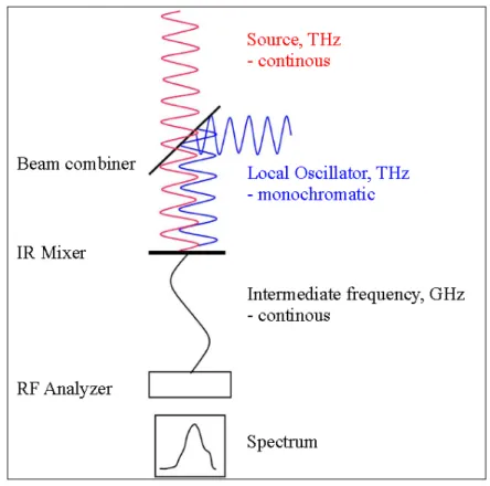
In a heterodyne receiver, the radiation emerging from the object to be analyzed is coherently superimposed to a well-known reference radiation provided by the so-called local oscillator (LO). Various beam combining elements can be used for superposition. Most commonly, beam splitters, Fabry-P´ erot resonators or waveg- uides are used. In the IR, waveguides are not as advanced yet, but first efforts were made towards a miniature IR heterodyne receiver using waveguides as beam combiner [56].

Figure 2.1: Schematic view on the heterodyne principle. Two planar EM-waves are

superimposed by a beam combining element. The spatial superposition is detected by

a photomixer which converts the THz radiation down to few GHz. The radio frequency

(RF) is then analyzed by standard RF components. From Stupar [41].

(25)

2.1 Heterodyne Technique 13

After superposition, the combined beam is detected by a detector, commonly called (photo-)mixer. The mixer must possess a non-linear characteristic in order to mix the high frequency signals from the source and the LO. Due to the mixing process, new frequencies of few GHz are generated. These frequencies can now be analyzed and processed using standard radio spectroscopic devices. The spatial superposition can be described by the summation of their electric fields E

_LO,sig

so that the electric field at the detector is

E

_det

= E

_LO

cos(ω

_LO

t + Φ

_LO

) + X

k

E

_sig,k

cos(ω

_sig,k

t + Φ

_sig,k

) (2.1) where ω

_LO,sig

is the output frequency of the LO and of the signal, respectively. It has to be noted, that the electric field of the signal E

_sig

consists of several spatial modes and thus has to be treated as the sum of the individual components k.

The incident power on the photomixer P

_det

is proportional to the intensity of the radiation I

_det

, which can be expressed as the square of the electric field

I

_det

∝ E

_det²

(2.2)

defining

P

_det

= 1 η

_q

hν

e

₀

I

_det

(2.3)

with

I

_det

= I

_LO

+ X

k

I

_sig,k

+ 2η

_het

X

k

p I

_LO

I

_sig,k

cos(kω

_LO

− ω

_sig,k

k t + 4Φ

_k

) (2.4) where 4Φ

k

is a constant phase shift between the LO and the signal. η

het

= η

q

+ η

mix

is the heterodyne efficiency, which takes the quantum efficiency of the detector η

_q

and optical losses, i.e. at the beam combiner, η

_mix

into account. The initial and the sum frequencies are to high and cannot be processed. They are represented by the DC components I

_LO

+ P

k

I

_sig,k

and result in an averaged photo current.

Only the difference frequency 4ω

_k

= kω

_LO

− ω

_sig,k

k between the detected signals, called intermediate frequency (IF) is detected. The IF spectrum contains all orig- inal spectral information. The spectral size of the IF spectrum depends on the bandwidth of the applied photomixer and is typically of few GHz.

Due to the symmetry of the cosine function two valid solutions for 4ω can be

found. All frequencies ω

_sig,k

< ω

_LO

originate in the lower side band (LSB), fre-

quencies ω

_sig,k

> ω

_LO

originate in the upper side band (USB) of the so-called

double side band (DSB) spectrum. In the resulting IF spectrum, a distinction

between LSB and USB cannot be made. The DSB is simply the sum of the in-

dividual contributions. In Fig. 2.2 the various steps from a direct detection to a

DSB heterodyne spectrum are illustrated.

(26)

Figure 2.2: Steps from a homodyne to a heterodyne spectrum. Top: the homodyne

spectrum of an atmospheric absorption feature in the THz region. Center top: The same

atmospheric feature divided into the LSB and USB. Center bottom: USB and mirrored

LSB in the IF bandwidth. Bottom: resulting heterodyned DSB spectrum in the IF

bandwidth.

(27)

2.2 Sensitivity 15

2.2 Sensitivity

Comparison of the sensitivity between heterodyne and direct detection methods is not trivial. A detailed investigation was made by Kr¨ otz [34]. In radio astronomy, the system temperature T

_sys

is commonly used to describe the noise equivalent power (NEP) of a heterodyne receiver. This notation allows the direct comparison of various heterodyne instruments and is adapted to infrared heterodyne receivers [55]. The NEP is the minimum detectable power with a given post detection bandwidth of 1 Hz and can be written in terms of T

_sys

as

N EP = s

8 δ

²_res

δ

_{f l}

k

_B

T

_sys

(2.5)

with the Boltzmann constant k

B

, the resolution bandwidth δ

res

and the fluctuation bandwidth δ

_{f l}

of the system. In order to characterize the resolution of an acousto- optical spectrometer (AOS, as used for signal analysis in the receiver, comp.

Subsec. 2.4.3) the Rayleigh criterion is conventional. It describes two monochro- matic frequencies as resolved, when the first maximum of the diffraction image of the second component coincides with the first null of the diffraction image of the first component. Their spectral distance is the fluctuation bandwidth δ

f l

[57].

2.2.1 System Temperature

The system temperature T

_sys

is convenient to characterize the noise of a heterodyne receiver. It has to be noted, that

T

sys

= T

ant

+ T

rec

(2.6)

divides into two components [58]. The antenna temperature T

_ant

is a measure for the noise of the detected signal and the transmission line. The receiver temperature T

_rec

in contrast, represents the intrinsic noise contribution, originating from the various devices of the receiver. It includes all losses in the instruments’ optics but mainly depends on the mean quantum efficiency η

_q

of the mixer. η

_q

describes the ratio of detected signal photons to generated electrons. Even in the ideal case of η

_het

= 1 (see Eq. (2.4)), a minimum noise contribution is indispensable. Hence, the ideal system temperature is limited by the so-called quantum limit. It can be written as

T

_ql

= h · ν

k

_B

(2.7)

(28)

where h is the Planck quantum and ν the observing frequency. The quantum limit T

_ql

represents the minimal system temperature for a purely shot noise limited receiver.

To determine the receiver temperature, two well-known reference signals are com- pared. In contrast to radio or sub-mm observations, the noise contribution of the transmission line’s thermal radiation is negligible. The incident power is directly proportional to the system temperature. Here, T

_ant

can be identified as the well defined surface brightness temperature of corresponding calibration sources, called hot H and cold C. The surface brightness temperature can be calculated accord- ing to Planck’s Law. Thus, the incident power of the calibration sources can be expressed as

H = α(T

_rec

+ T

_H

) and C = α(T

_rec

+ T

_C

) (2.8) where α is the unknown amplification of the system. The ratio of the incident power Y =

^H_C

terminates the dependency on the amplification and reveals the receiver temperature:

T

_rec

= T

_H

− Y · T

_C

Y − 1 . (2.9)

It is crucial to generate a high contrast between the two calibration signals. In IR heterodyne receivers, the hot load is usually a blackbody radiator, whereas the cold load is an absorber at room temperature.

2.2.2 Radiometer Equation and Noise Amplitude

An important parameter to describe the sensitivity of a heterodyne receiver is the noise amplitude. To retrieve information on the noise amplitude, analysis of the signal’s variance is important. A frequency independent noise amplitude is common for white noise. The radiometer equation describes the decrease of the frequency independent noise amplitude of a constant signal in time:

σ

²

(τ) = T

sys

p δ

_{f l}

· τ (2.10)

where σ

²

is the root mean square error (RMS) in K, T

_sys

is the system temperature, δ

_{f l}

is the fluctuation bandwidth of the back-end filter [59].

To obtain the resulting spectrum, the ratio of the incident signals from all observed sources is determined (comp. Eq. (2.8)):

F = S − R

H − C (2.11)

(29)

2.3 Line Broadening Effects 17

with H: hot calibration load, C: cold calibration load, S: sky signal, R: sky ref- erence. The radiometer equation Eq. (2.10) is valid for the integration on each source. To optimize the signal-to-noise ratio (SNR) it is necessary to minimize the RMS of the retrieved spectrum in Eq. (2.11), which can be calculated according to the error propagation law. Thus, as shown in Appendix A the RMS can be expressed in dependence on the whole exposure time τ and the temperature of the observed sources:

σ

²

(τ, F ) = T

_rec

p δ

_{f l}

τ · T

_S

+ T

_R

+ F (T

_H

+ T

_C

) T

H

− T

C

(2.12) For more information on the sensitivity of a heterodyne receiver please also refer to Abbas et al. [60], Schm¨ ulling [61] and Kr¨ otz [34].

2.3 Line Broadening Effects

For the investigation of absorption features, it is essential to understand the pro- cesses, responsible for the shape of the observed molecular transition lines. In the following the basic effects, leading to a broadening of spectral lines are discussed.

The descriptions below are following along the lines of Bernath [62].

The energy of photons traveling through a group of molecules can be either ab- sorbed or induce stimulated or spontaneous emission. Considering a finite volume of molecules and an incident photon flux, Beer’s law describes that the intensity of the incident radiation I

0

abates exponentially with distance l and can be described as

I(l) = I

₀

e

^−αl

(2.13)

where α the so-called absorption coefficient in cm

⁻¹

and is depending on the ab- sorption cross-section of the molecule and its concentration in the probed vol- ume.

The rotational structure of a dipole, vibrating in a particular mode, is called

band. These rotational-vibrational (ro-vibrational) bands are composed of single

transitions, called lines. A typical molecular spectrum of the CO

₂

antisymmet-

ric stretching mode is illustrated in Fig. 2.3. To resolve one single ro-vibrational

transition, ultra high frequency resolution is required. Usually, the shape of these

lines can be described by line-shape functions, which are classified into homoge-

neous and inhomogeneous functions. The distinction is due to the properties of

the molecules. A homogeneous line shape occurs, when all molecules are subject

to equal ambient conditions, i.e. the surrounding pressure. Consequently, an inho-

mogeneous line shape is assumed for varying molecular properties, i.e. the velocity

(30)

Figure 2.3: A typical molecular spectrum of the antisymmetric stretching mode of CO

₂

. One vibrational mode contains a complete band of rotational transitions. In the insert graphic, one ro-vibrational transition line is shown in absorption. From Bernath [62]

of the single molecules which is Maxwell-Boltzmann distributed. This broadening effect is called Doppler-broadening.

2.3.1 Natural Lifetime Broadening

Each molecular transition possesses an intrinsic broadening effect, which is due to the finite lifetime (τ

LT

) of the excited energy level. This effect is called nat- ural lifetime broadening. In quantum mechanics, the energy state of a molecule is described by a time-dependent wavefunction. The Fourier transformation of an infinite wavefunction yields the frequency of the wave as a sharp delta peak.

However, since the excited state decays into a lower state by spontaneous emission after a while, a finite lifetime of the excited state exists and the wavefunction is not infinite. The Fourier transformation of a transition with a certain decay rate gives the homogeneous line-shape function. The function represents a statistical distribution around the centroid frequency and can be described by a Lorentzian function with a full width at half maximum ( Fwhm ) given by

4ν

_Fwhm

= 1

2πτ

_LT

(2.14)

(31)

2.3 Line Broadening Effects 19

This Fwhm is often called natural line width and can also be regarded as a con- sequence of the Heisenberg uncertainty principle.

2.3.2 Pressure Broadening

Pressure broadening occurs due to collisions between molecules and is thus also called collisional broadening. To understand the process, we consider a transition from a higher to a lower state, which can be described by a wavefunction. The dipole moment of the molecule oscillates at a certain frequency except for time of collision. Then, the wavefunction is disrupted and the dipole moment is altered.

This disruption leads to a finite length of the wavefunction and the Fourier trans- formation of the divided wave yields, similar to the natural lifetime broadening, a homogeneous line-shape function, which can be described by a Lorentzian distri- bution. The Fwhm of the curve is proportional to the reciprocal of the average time T

_c

between two collisions. Increasing the ambient pressure, decreases the time between two collisions. Hence, the Fwhm of the line can be given in terms of the pressure as

4ν

_Fwhm

= b · p (2.15)

where b is identified as the substance-specific pressure-broadening coefficient. The encounter of two molecules is depending on the interaction of their potentials, and cannot be exactly determined in a group of three or more, thus, the derivation of the pressure-broadened line shape is a difficult task and the pressure-broadening coefficients are experimentally determined. For CO

₂

, the self-broadening coeffi- cient is ∼ 7.6 MHz/Torr [63].

2.3.3 Doppler-Broadening

Gas in a finite volume contains a certain amount of molecules, which are all mov- ing in a different direction. This varying motion of the molecules provokes a small scale frequency shift of the incident radiation, resulting in many, natural lifetime broadened homogeneous line shapes. The envelope of this set of lines is an in- homogeneously broadened line and can be described by a Gaussian distribution (comp. Fig. 2.4). The Fwhm of the Doppler-broadened line is depending on the mass m of the molecules at a given temperature T and can be written as

4ν

_D

= ν

₀

c

r 8k

_B

T ln(2)

m (2.16)

where ν

₀

is the centroid frequency of the line, c is the speed of light and k

_B

the Boltzmann constant. From Eq. (2.16) the kinetic temperature of the observed

(32)

Figure 2.4: An inhomogeneously broadened line (Gaussian distributed) made up of many homogeneously broadened components (Lorentzian distributed). From Bernath [62]

molecule can be retrieved, if the width of the line is given. Hence, fitting a Gaussian function to a purely Doppler-broadened line shape reveals the kinetic temperature of the molecule.

In case the molecules are subject to both broadening mechanisms, the result- ing line-shape function must be described as a convolution of a Gaussian and a Lorentzian distribution function. This convolution is called Voigt line-shape func- tion.

In planetary atmospheres, the pressure decreases with altitude, since the molecules are gravitationally forced towards the surface. The line forms either between the surface or the altitude, where the pressure is low enough for the atmosphere to be not optically thick anymore and the altitude where the pressure is high enough for the pressure broadening to exceed the Doppler broadening. In this region, the energy emerging from the background radiation source, is absorbed and re-emitted as traveling along the path of ray. Therefore, one Voigt profile is not sufficient to describe an atmospheric absorption line. Thus, a full radiative transfer calculation has to be performed, which accounts for the varying pressure in the atmosphere.

Details on the radiative transfer code I used for the work herein are given in the next chapter, Chap. 3.

2.4 Instrumentation

Infrared heterodyne spectrometer are still rare and only few instruments exist

worldwide. The first heterodyne receiver was developed at the University of Cali-

fornia (UC) in Berkeley in the early 1970s, to measure CO

₂

emission lines in the

atmosphere of Mars and Venus [64–67]. The biggest instrument nowadays that uti-

(33)

2.4 Instrumentation 21

lizes the IR heterodyne method is the Infrared Spatial Interferometer ( Isi ), which was developed by the group of the UC Berkeley around Betz, Johnson and Towns [68]. Isi is a high spatial resolution interferometer, consisting of three movable 1.65 m telescopes. Each of them heterodynes the incoming radiation with a CO

₂

laser emission [69]. The combination of interferometry and heterodyning creates a unique way to achieve high spatial and spectral resolution. Isi ’s main field of application, however, is the investigation of stellar environments [69].

In middle of the 1970s a group at the Nasa Goddard Space Flight Center de- veloped the Infrared Heterodyne Spectrometer ( Irhs ), used for planetary obser- vations in the mid-IR wavelength region [70, 71]. At first, it was permanently mounted at the Mc-Math Pierce Solar Telescope (McMath) in Arizona, USA, be- fore it was relocated to the Nasa Infrared Telescope Facility ( Irtf ) on Hawaii.

At the end of the 1990s, the instrument was disassembled and substituted by the newer and more flexible Heterodyne Instrument for Planetary Winds And Com- positions ( Hipwac ) [72]. Hipwac was the first transportable infrared heterodyne receiver in the world.

Around the beginning of the century, a second transportable instrument, the Cologne Tuneable Heterodyne Infrared Spectrometer ( This ), was assembled. The instrument is in operation since 2002 [73, 74].

In recent years, more mid-infrared heterodyne receivers were developed. In Cologne, a second instrument called i Chips (infrared Compact Heterodyne Instrument for Planetary Science) was built, intended as a breadboard for laboratory measure- ment and terrestrial observations [51]. In addition, a Japanese group is about to start observations with their newly developed instrument at the Planets tele- scope on Haleakala, Hawaii [75]. Besides the mid-IR receivers, a couple of near-IR instruments exist and have been successfully applied for observations. However, these instruments are less advanced and have mainly been used for terrestrial observations [76, 77].

This and Hipwac are still operating and have been used for the observations

within this thesis. In the following, they will be presented in more detail. A

description of the receivers setup and most important components is given for each

instrument, to point out the major differences and commonalities. An overview

of some characteristics and specifications can be found at end of the chapter in

Tab. 2.2.

(34)

2.4.1 THIS

Spectrometer Setup

The beam path in This is displayed in Fig. 2.5. A picture of the receiver is shown in Fig. 2.6(a). The instrument was designed to fit in a two-story aluminum frame- work. The receivers dimensions are 80 x 60 x 42 cm

³

and it weighs approximately 80 kg. The inner part of the cube is indicated as the LO deck in the scheme in

Figure 2.5: Schematic view on the beam path in This . The broadband IR signal

(green) coming from the various radiation sources is injected into the spectrometers

optical path by a high speed galvano scanner. The radiation from the sky is split into

its optical (light blue) and its IR component by a dichroic mirror. The optical light is

detected by a CCD for guiding purposes. The IR signal is fed into the diplexer and

heterodyned to the LO beam (blue). A fraction of the LO power is routed through a

reference gas cell onto a MCT (HgCdTe) detector to monitor the output frequency of

the LO. A stabilized HeNe laser (red) is also injected into the diplexer in order to lock

the LO frequency onto a specific resonator fringe. (Sonnabend et al. [55])

(35)

2.4 Instrumentation 23

(a) This : dimension 80 x 60 x 42 cm

³

(b) Hipwac : dimension 75 x 80 x 137 cm

³

Figure 2.6: Photos of the two receivers.

Fig. 2.5. The LO deck contains the beam combining optics, the detector and the LO. In addition, all components required for frequency stabilization are mounted inside the LO deck. The upper part of the receiver contains all the optics nec- essary for matching the instrument to different telescopes with different F# [55].

It is marked as the signal deck in Fig. 2.5. Besides the IR signal and calibration components, an indispensable optical guide system is located on the signal deck.

All electronic components, needed for operation are mounted into two separate 19” racks which makes it convenient for transportation and handling.

The Local Oscillator - QCL

This is the first infrared heterodyne receiver that uses quantum cascade lasers

(QCLs) as LO. QCLs are semiconductor lasers and have been developed in 1994

by Faist et al. [78]. In these types of lasers, photon emission is obtained by op-

tical transitions of electrons between confined energy levels [79]. The transitions

take place between intersubbands in a multi-quantum-well structure. In Fig. 2.7

the scheme of a QCL with the concept of alternating wells and barriers is on

display.

(36)

Figure 2.7: Energy diagram of a QCL from Yao et al. [80]. The laser transition takes place in the active region between sub-band 3 and 2. The sub-bands contain alternating structure of quantum-wells and barriers in order to force stimulated emission.

The advantage of QCLs compared to other lasing devices, i.e. diode lasers, are their high continuous wave (CW) output power and spectral tuning range. A QCL is a multi layer semiconductor usually made out of GaInAs/AlInAs heterostructures.

The emission frequency of the laser is depending on the layer structure and can be tailored over a wide range by changing only the thicknesses. Hence, a mani- fold of QCLs are available in the mid-IR wavelength regime between 3 µm–25 µm [80]. However, two kinds of QCLs have to be distinguished. The multi-mode Fabry-Perot (FP) devices and the distributed feedback (DFB) QCLs. DFB-QCLs possess an incorporated internal grating which allows monochromatic single-mode operation with a narrow linewidth [81, 82]. Despite the narrow linewidth, DFB- QCLs provide a spectral tuning range of approximately 1% around the central wavenumber [78]. Tuning of the device can be achieved by either changing the ap- plied current or the operation temperature. The former results in a fast, the latter, due to a longer thermal relaxation time, in a slow tuning effect. This provides a

# λ

peak

tuning range operating temperature

µm cm

⁻¹

µm cm

⁻¹

K

1 10.54 948.63 10.51–10.57 947–951.5 187–243

Table 2.1: QCL mounted in This during observations for this work.

(37)

2.4 Instrumentation 25

common tuning range of 6–10 cm

⁻¹

. Initially, QCLs had to be liquid nitrogen (LN) cooled to be operated at low temperatures. In recent years, the development was successfully driven towards devices that could be operated at room temperature [79]. LN cooled DFB-QCLs are used in This . Mostly, the devices are heated addi- tionally, in order to increase their tunability. A list of the important parameters of the device used in This during observations for this work is given in Tab. 2.1.

The Beam Combiner - Diplexer

A confocal FP ring resonator, called diplexer, is used as the beam combining element. Two focusing mirrors, with a focal length of 30 mm each, are placed in the respective opposed focal spot. The beams are injected into the resonator through two highly reflective beam splitters. The transmission in the diplexer follows the Airy function and, assuming a good alignment, the maxima are separated by 4ν = c/2 · l, with l the length of the resonator. The suppression of side modes from the QCL and the avoidance of accidental reflective feedback are two advantages of the setup. To assure optimal amplification in the cavity, one mirror can be modulated by a piezo actuator at a frequency of a few hundred Hz. This way, the diplexer can serve also for frequency stabilization purposes. The LO can be stabilized to the maximum of a resonator fringe with an accuracy of ∼ 1 MHz. Further information can be found in the work of Wirtz [83], Sonnabend [73], Sonnabend et al. [55] and Sornig [84].

Beam Selection and Signal Calibration

In Sec. 2.2.2, we learned from Eq. (2.11), that for obtaining a calibrated spectrum it is necessary to observe four different input signals. To select the different radiation sources a galvano scanner is implemented into the spectrometer (comp. Fig. 2.5).

The scanner switches between the calibration loads Hot, Cold and the beam from

the sky provided at the on-source Signal and the off-source Ref erence port. In

THIS, the hot load is a black body radiation source at 673 K and the cold load a

room temperature absorber. In addition, a steady state emitter, observed through

a reference gas cell, is introduced as a fifth source, required for monitoring the

frequency position and stabilization of the LO. The galvano scanner enables high

speed switching between the various positions within only a few milliseconds. It

injects the required broadband signal beam by rotating into the accurate angular

position. Its high switching frequency can be precisely synchronized with the

observing procedure. This enables the measuring of the loads and the source

within the short period of one observing cycle.

(38)

2.4.2 HIPWAC

Spectrometer Setup

The setup of Hipwac is displayed in Fig. 2.8 and a picture of the instrument can be found in Fig. 2.6(b). The size of the receiver is 75 x 80 x 137 cm

³

. It weighs approximately 90 kg. In contrast to THIS, the optical components in Hipwac

Figure 2.8: Schematic view on the beam path in Hipwac . The broadband signal

coming from the sky is split into its visible (light blue) and its IR (green) component by

a dichroic mirror. The visible light is detected by a CCD for guiding purposes. To select

the hot load, a flip mirror can be introduced into the beam path. A chop between the

hot and the cold load is achieved by a chopper wheel. The IR signal is superimposed

to the LO beam (blue) on a beam splitter. The LO output power can be reduced in

the attenuator. By removing a flip mirror, the LO output frequency can be monitored

in a spectrum analyzer. The heterodyned beam is detected by the IR mixer and finally

analyzed. (Stangier 2014 [52])

(39)

2.4 Instrumentation 27

are vertically aligned and the two decks are mounted to the opposed sides of an upright optical plate. The receivers framework is made of carbon fibers. The LO deck contains the LO, an attenuator and a spectrum analyzer. On the signal deck the calibration loads, the beam combining element and an optical guide system are located. In addition, the optical components which are needed for telescope adaption can be found on the signal deck. The broadband signal coming from the sky is fed into the instrument from the top, through a hole in the lid. The IF signal provided by the mixer can not only be analyzed with an AOS, but also with a high-resolution filter bank [45], which is omitted in the scheme in Fig. 2.8, since it was not used for data acquisition in this work.

The Local Oscillator - CO

₂

Gas Laser

In Hipwac the LO signal is provided by a CO

2

gas laser. In order to increase the spectral coverage of the instrument, two different laser gain tubes can be selected. Each laser gain tube contains different CO

₂

isotopes, yielding a manifold of transitions around the

¹²

C

¹⁶

O

2

I-, and II-band centered at 10.4 µm and 9.4 µm, respectively. The desired transition can be selected by tuning the cavity length of the gain tube. This can be achieved by changing the angle of incidence of an incorporated diffraction grating on one end of the tube. In gas lasers, though, tunability is limited and the monochromatic LO output frequency is restricted to a small bandwidth around the energy peak of the specific transition. To guarantee a stable output frequency, the laser is locked to the peak of the gain profile [85].

The advantage of CO

₂

gas lasers is their high output power. To ensure a con- stant power for the various transitions and to avoid signal saturation on the back- end detection devices an attenuator is introduced in the LO beam path (comp.

Fig. 2.8). The spectrum analyzer serves for monitoring the selected transition of the laser.

Beam Selection and Signal Calibration

Hipwac cannot be applied as flexible as This . Since it is not equipped with an appliance to switch between signal and reference, the instrument must rely on telescopes which are capable of chopping the beam on the sky, e.g. the Irtf . The hot load can be observed by introducing a flip mirror into the beam path. The flip mirror is electronically controlled in order to obtain a calibration measurement remotely. A chopper wheel is then used to chop between the hot and the cold load.

The cold load in Hipwac is represented by the filled areas of the chopper wheel,

which are kept at room temperature. The hot load is a black body radiator with

(40)

a surface temperature of 1273 K. In Hipwac the calibration procedure cannot be implemented into the observing procedure as it is in This . Therefore, it has to be done after each measuring cycle.

The various broadband signals are heterodyned to the LO signal on the beam combining element, which is a 2 x 3 inch

²

ZnSe beam splitter. The beam splitter has a special IR coating which reflects 10 % and transmits 90 % of the signal.

THIS HIPWAC

Local oscillator QCL CO

2

-Laser

Operating wavelength 7.8–11.2 µm (tunable) ∼ 10 µm (CO

₂

-band)

Beam combiner Diplexer Beam splitter

Receiver Dimensions 80 × 60 × 42 cm

³

, 80 kg 75 × 80 × 137 cm

³

, 90 kg AO-Spectrometer 3 GHz, 6000 channels 1.6 GHz, 3000 channels

Spectral Stability ∼ 0.3 MHz ≤ 0.01 MHz

Maximum Resolution

_∆ν^ν

≥ 10

⁷

, adjustable

Sensitivity T

sys

≤ 3000 K at 10 µm

Table 2.2: List of important specifications for This and Hipwac .

2.4.3 IR Mixer and AOS

Both instruments use an mercury-cadmium-telluride (HgCdTe or Mct ) IR de- tector. In each case, it is a doped semiconductor pin-photodiode optimized for heterodyne detection between 7.6 µm and 12.0 µm. It consists of four single detec- tor chips, each of them embodies one pin-photodiode buried in an optical cavity.

The incorporated resonator creates a standing wave pattern within the HgCdTe material to optimize sensitivity of each chip to different wavelengths [86]. The resonator increases the quantum efficiency η

_q

to ∼ 80 %. The photomixers have to be LN cooled and their 3 dB cutoff is at ∼ 3 GHz.

The back-end spectrometers used for signal analysis are AO-spectrometers. AOS were developed and assembled at our institute [57] and have been applied success- fully for various purposes in the field of radio-astronomy and spectroscopy for many years [74, 87, 88]. The two AOS applied in the instruments are slightly different.

Both possess a fluctuation bandwidth δ

_{f l}

of 1.3 MHz. The AOS used in This has an IF bandwidth B of 3 GHz, the one in Hipwac of 1.5 GHz, respectively, limiting the IF bandwidth of the entire instrument.

In an acousto-optical spectrometer, the IF photons of the signal to be analyzed,

excite grating vibrations of a Bragg crystal. These vibrations modulate the refrac-

(41)

2.4 Instrumentation 29

tive index of the crystal. A laser beam is routed through the crystal and collimated onto a linear CCD. This enables the simultaneous detection of the broadband IF signal, since the modulated dispersion of the crystal, caused by the spectral dis- tribution of the IF, leads to a spatial refraction of the AOS laser. The amount of channels of the CCD defines the bandwidth B of the AOS. In This , the AOS-CCD has 6000 channels and in Hipwac 3000, respectively. For more detailed informa- tion on the functionality of an AOS, please refer to the work of Schieder et al. [57], Siebertz [89] or Olbrich [90]. Further analysis and data processing is performed by a PC.

2.4.4 Spectral Stability

One important factor for observations requiring long integration times is the spec- tral stability of the receiver. The importance even increases for ultra high spectral resolution. To claim a spectral resolution of ∼ 1 MHz is only valuable, if the spec- tral stability is guaranteed to be less or equal to this value. The spectral stability of the AOS can be assumed as given, as it was proven several times in the past [57, 89, 90]. Additionally, a comb generator with defined spectral distance of 50 MHz between the comb emission lines, is implemented into the IF processing box in order to calibrate the AOS-CCD precisely. Hence, all potentially slow and long term drifts of the back-end spectrometer, caused by varying ambient temper- atures can be ruled out.

In This , the spectral stability was tested by observing a well known molecular transition feature of a reference gas in absorption. The pressure of the gas must be low enough to obtain an only Doppler-broadened line shape. Commonly, a pressure of less than ∼ 5 hPa is sufficient [55]. A Gaussian distribution is fitted to the absorption line, yielding the IF center frequency of the feature. The procedure was repeated every 30 s for 4500 s, simulating real observing conditions. A typical result of such a stability measurement is shown in Fig. 2.9. The obtained standard deviation of the IF frequency position of the line, which directly correlates to the output frequency stability of the LO, is 0.3 MHz. The slight slope, that can be observed in Fig. 2.9(b) is due to the thermal properties of the QCL. However, these long term drifts can be neglected, since an absorption line is frequently measured during the observing procedure, for LO frequency calibration purposes.

In Hipwac , an additional load for monitoring the spectral stability of the receiver

is abdicated. The CO

₂

gas lasers are assumed to provide a stable output frequency

over the observing period. The laser can only emit at the rest frequency of the

selected transition to which it is locked. The transition is selected by changing

(42)

(a) (b)

Figure 2.9: Spectral stability of This from Sonnabend et al. [55]. IF line center frequency variation over time. The inset values in (b) are the mean value and the standard deviation (SD) given in MHz.

the resonator length. The rest frequency is independent from external parameters such as ambient pressure or temperature. The resonator length however, can vary due to external influences and must be stabilized to keep the output frequency constant. This is achieved by a piezo actuator, controlling the incorporated grating at the end of the laser gain tube. Hence, the LO output frequency can only be slightly tuned within a small bandwidth around the very narrow emission peak of less than 10 kHz. This can only result into a potential frequency drift which is two magnitudes smaller than the resolution bandwidth of the AOS and thus negligible.

In case of a major deviation, the stabilization circuit would be truncated and the incident would be indicated on the electronic control rack.

2.4.5 Allan Variance Measurement

A key factor for astronomical and terrestrial observations is the amplitude stability

of the receiver. Its variance, σ, must decrease with increasing integration time, τ

(comp. Eq. (2.10), radiometric behavior) [91]. The Allan variance method, a com-

mon procedure to investigate the accuracy of time and frequency standards [92],

is used to demonstrate the radiometric decrease of the noise amplitude. The mini-

mum of the Allan variance can be determined using a power law, where frequency

drifts are proportional to τ

^β

and the white noise contribution is proportional to

¹_τ

(43)

2.4 Instrumentation 31

[93]. It can be written as:

σ

²_A

(τ ) = a

τ + bτ

^β

with β ≥ 1 (2.17)

Hence, when the variance is plotted on a logarithmic scale, the −1 slope defines the time interval in which the radiometer equation must be valid and only white noise contributes to the spectrum. This time interval can be individually determined for each receiver and defines the maximal integration time for one cycle τ

_cyc

, the so-called Allan-time. During that time, all individual sources need to be observed.

To obtain the resulting spectrum, the single cycles are stacked, conserving the pure

white noise contribution. In This the Allan-time is ∼ 60 s [73].

(44)

Atmospheric Thermal Properties of Venus and Mars -