Observations of Upper Mesosphere Temperatures on Venus and Evaluation of Mid-Infrared Detectors for the Tuneable Heterodyne Infrared Spectrometer (THIS)

(1)

Observations of Upper Mesosphere Temperatures on Venus

and

Evaluation of Mid-Infrared Detectors for the Tuneable Heterodyne Infrared Spectrometer

(THIS)

I n a u g u r a l - D i s s e r t a t i o n zur

Erlangung des Doktorgrades

der Mathematisch-Naturwissenschaftlichen Fakultät der Universität zu Köln

vorgelegt von Peter Krötz aus Karlsruhe

im Mai 2010

(2)

Prof. Dr. R. Schieder Prof. Dr. S. Crewell

Tag der mündlichen Prüfung: Juli 2010

(3)

List of Figures

2.1 THIS schematic . . . . 11

2.2 Diplexer Transmission . . . . 12

2.3 AOS schematic . . . . 13

2.4 QCL principle . . . . 14

2.5 THIS: present wavelength coverage . . . . 16

2.6 Detector stability . . . . 18

2.7 Detector stability . . . . 19

2.8 THIS . . . . 20

2.9 HIPWAC . . . . 23

2.10 Direct vs Heterodyne detection: signal-to-noise ratios 28 3.1 Model of Venus’ Thermosphere . . . . 31

3.2 PVO T-Profile . . . . 33

3.3 Sub-mm measurements of CO . . . . 35

3.4 CO line centre variations . . . . 37

3.5 CO 2-1 observations . . . . 38

3.6 Temperatures from O

2

air-glow . . . . 39

3.7 Venus Express: VIRTIS . . . . 41

3.8 Venus Express: SPICAV . . . . 43

3.9 Venus Express: VeRa . . . . 44

3.10 Non-LTE emission: population inversion . . . . 47

3.11 VIRTIS: non-LTE altitude . . . . 48

3.12 Modelled non-LTE emission altitude . . . . 48

4.1 THIS Spectrum . . . . 52

4.2 Temperatures March 2009 . . . . 53

4.3 Temperatures April 2009 . . . . 55

iii

(6)

4.4 Temperatures June 2009 . . . . 56

4.5 HIPWAC spectrum . . . . 59

4.6 Temperatures HIPWAC 2007 . . . . 60

4.7 All observed lines in the 10.6 µm P-branch . . . . 61

4.8 Line Intensities . . . . 63

4.9 Temperatures retrieved along the Equator . . . . 64

4.10 IRHS Spectrum . . . . 67

4.11 IRHS Temperatures 1990 . . . . 69

4.12 IRHS Temperatures 1991 . . . . 70

5.1 Venus polar vortex . . . . 73

5.2 Variations at Equator / Limb . . . . 74

5.3 Temperatures at Limb (June ’09) . . . . 75

5.4 IC 2009: Temperature Symmetries . . . . 77

5.5 ICs 1990/91: Temperature Symmetries . . . . 78

5.6 Comparison of ICs 1990/91 / 2009 . . . . 80

5.7 Sub-mm observing Geometry . . . . 81

5.8 Inter heterodyne comparison . . . . 82

5.9 Solar Cycles 19-24 . . . . 83

5.10 Simultaneous Observation Sub-mm / IRHet: Equator 85 5.11 Simultaneous Observation Sub-mm / IRHet: Equator 85 5.12 Simultaneous Observation Sub-mm / IRHet: South Pole 86 5.13 Sub-mm observing Geometry . . . . 88

5.14 Comparison: THIS/sub-mm at max. elongation . . . 89

5.15 Long-term mm observations . . . . 90

5.16 Venus Atmosphere: IC Model . . . . 93

5.17 IC Model (2) . . . . 94

5.18 Comparison to VTGCM . . . . 95

6.1 Zeeman splitting of Solar lines . . . . 100

6.2 Telluric Ozone Absorption against Betelgeuse . . . . . 106

7.1 Optics transmission I . . . . 108

7.2 Optics transmission II . . . . 108

7.3 17 µm laser emission . . . . 109

7.4 MCT material dependence . . . . 110

7.5 Long wavelength reference detector . . . . 111

(7)

LIST OF FIGURES v

7.6 THIS - MCT . . . . 112

7.7 Comparison JMCT RMCT . . . . 114

7.8 Power meter absorption . . . . 115

7.9 MCT temperature dependence . . . . 116

7.10 RMCT resistance . . . . 116

7.11 RMCT @ 9 µ m . . . . 117

7.12 RMCT @ 13 µ m . . . . 117

7.13 RMCT @ 17 µ m . . . . 118

7.14 QCD schematic . . . . 119

7.15 Quantum cascade detector . . . . 120

7.16 QCD illumination . . . . 120

7.17 QCD responsivity . . . . 121

7.18 Pulsed QCD response . . . . 122

(8)

4.1 Results March 2009 . . . . 54

4.2 Results April 2009 . . . . 55

4.3 Results June 2009 . . . . 57

4.4 Results IRTF 2007 . . . . 62

4.5 Comparison rotational / kinetic temperature . . . . . 63

4.6 Kinetic temperatures along the equator . . . . 65

4.7 IRHS observing campaigns . . . . 66

4.8 IRHS: temperature results . . . . 68

5.1 Comparison rotational / kinetic temperature . . . . . 71

6.1 THIS sensitivity characteristics at 17 µ m . . . . 105

7.1 MCT response . . . . 113

vi

(9)

Abstract

Infrared heterodyne spectroscopy today is an inherent part in plan- etary atmosphere observations. It is based on the superposition of the observed signal to a local oscillator and provides highest possi- ble spectral resolution. Non-thermal emission of CO

2

in the upper mesosphere of Venus was discovered by the NASA Infrared Hetero- dyne Spectrometer (IRHS) in the 1970s and was repeatedly target of observations since then. In the course of this thesis, data of with IRHS, its successor HIPWAC and the Cologne Tuneable Heterodyne Infrared Spectrometer (THIS) was taken or analysed. From the mea- sured line widths the kinetic temperature of the atmosphere at the emission altitude of around 115 km could be determined.

Observed temperatures are generally higher than predicted by the Venus International Reference Atmosphere (VIRA). VIRA is a empir- ical model mainly based on data of the Pioneer Venus space mission and exhibits only a limited data set.

Other ground-based observations as well as results from Venus Ex- press confirm the warm atmosphere at similar altitudes. At the day side of Venus and at this specific altitude, infrared heterodyne spec- troscopy is currently the only method to observe temperatures.

Another result is the high variability of the observed atmosphere which is not expected by the VIRA model but which was also seen in earlier mm-wavelength observations. The obtained results also set new constraints for modern global circulation models. Improv- ing those models will lead to a improved knowledge of planetary at- mospheres. As all those models are based on the Earth atmosphere model, our observations might subsequently lead to a better under- standing of the terrestrial climate as well.

The second part of this thesis deals with the evaluation of possi- ble detectors for THIS to expand the wavelength coverage to longer wavelengths. Many atomic and molecular lines could be targeted within the solar system and beyond. The main target will be cold molecular hydrogen in the interstellar medium which is of highest importance in astrophysical questions concerning star forming, dark matter and cosmology. For this reason first tests at 17 µm wavelength were done in the course of this work.

1

(10)

Infrarot Heterodyn Spektroskopie hat heute ihren Platz in der Planetenbeobachtung gefunden. Sie beruht auf der Überlagerung des beobachteten Signals mit einem Lokaloszillator und bietet höchstmögliche spektrale Auflösung. Nicht-thermische CO

2

Emis- sion in der oberen Mesosphäre der Venus wurde mit dem Infrared Heterodyne Spectrometer (IRHS) des NASA Goddard Space Flight Centers entdeckt, und seit den Siebziger Jahren des vergangenen Jahrhunderts regelmäßig beobachtet. Daten von IRHS, dem Nach- folgegerät HIPWAC (Heterodyne Instrument for Planetary Wind and Composition) und dem Kölner Spektrometer THIS (Tuneable Heterodyne Infrared Spectrometer) wurden im Rahmen dieser Arbeit aufgenommen, bzw. ausgewertet. Anhand der Linienbreite der CO

2

-Emission konnte die kinetische Temperatur der Venusat- mosphäre in einer Höhe von circa 115 km bestimmt werden.

Im Vergleich zur Venus Referenzatmosphäre (VIRA, Venus Interna- tional Reference Atmosphere) sind die erhaltenen Temperaturwerte deutlich höher, um bis zu 50 K. VIRA wurde empirisch anhand von Satellitenmissionen (hauptsächlich die Pioneer Venus Mission) erstellt und weist an vielen Stellen nur einen unzureichenden Datensatz auf.

Andere bodengebundene Beobachtungen sowie Experimente an Bord des aktuellen Orbiters VenusExpress bestätigen die tendenziell wärmere Venusatmosphäre in vergleichbaren Höhen. Infrarot Heterodyn Spektroskopie ist allerdings die einzige Methode um die Temperaturen in dieser Höhe auf der Tagseite und mit hoher räumlicher Auflösung zu messen.

Aus einzelnen Meßkampagnen sowie im Vergleich mit anderen Messungen ergibt sich ein extrem variables Bild der Venus Atmo- sphäre in 115 km Höhe. Dies war laut VIRA nicht zu erwarten und stellt Ansprüche an neue Atmosphärenmodelle. Da sich die Modelle der Planetenatmosphären in der grundlegende Physik nicht unterscheiden können Verbesserungen des Venusmodells auch dazu beitragen das Verständnis physikalischer Vorgänge in der Erdatmosphäre und somit der Entwicklung des Erdklimas zu verbessern.

Weiterhin war es Ziel dieser Arbeit, den Wellenlängenbereich des THIS Spektrometers zu längeren Wellenlängen zu erweitern. Zahlre-

2

(11)

iche Molekül- und Atomlinien könnten so in Planetenatmosphären und auch extrasolar beobachtet werden. Das Hauptziel dabei ist die Beobachtung von kaltem molekularen Wasserstoff im interstellaren Medium. Wasserstoff ist der grundlegende Baustein des Univer- sums, zahlreiche Fragen der Kosmologie, z.B. die nach der dunklen Materie, oder der Sternentstehung sind mit der Verteilung und der Häufigkeit von Wasserstoff verknüpft.

Erste Labortests bei 17 µm Wellenlänge sowie eine Evaluierung

geeigneter Detektoren wurden dazu durchgeführt.

(12)

(13)

Chapter 1

Infrared Heterodyne Spectroscopy:

Research and Development

Infrared Heterodyne (IRHet) Spectroscopy fills a niche in today’s as- tronomical instrumentation. Its characteristics - ultra high spectral resolution over a relatively small bandwidth - call for very distinct science applications.

While heterodyne techniques are state of the art at radio and THz frequencies, observations in the infrared atmospheric windows are dominated by direct detection systems.

In the mid 1970s a group at the NASA Goddard Space Flight Center (GSFC) near Washington D.C. started to develop an Infrared Heterodyne Spectrometer (IRHS) which later was redesigned and upgraded to the Heterodyne Instrument for Planetary Wind And Composition (HIPWAC). Together with the Cologne Tunable Heterodyne Infrared Spectrometer (THIS) these two instruments today are the only ones applying heterodyne techniques in the mid-infrared.

The mid-infrared around wavelengths of 10 µ m is a transition zone, where one has to decide which technique is more favourable. If high spectral resolution is not needed, direct detection can provide higher sensitivities. For some applications, however, the ultra high

5

(14)

spectral resolution of heterodyne spectroscopy is needed. The key science application from the beginning of IRHet was the observation of planetary atmospheres, more precisely of planetary atmosphere dynamics. There, spectral resolution of more than 10

⁵

( ν/δν ) is mandatory.

In this thesis IRHet observations are analysed for mesospheric tem- peratures for the first time. Therefore, temperature dedicated ob- serving runs with the instruments THIS and HIPWAC are analysed as well as old IRHS data, taken in 1990 and 1991. These data are ex- tremely valuable for the verification of global circulation models of planetary atmospheres, which recently developed very fast thanks to data from orbiters like Mars- and VenusExpress. A better under- standing of atmospheres around other planets will ultimately also increase the knowledge about our own atmosphere and help to re- fine models on climate change. In this way, observations of tempera- tures in the upper mesosphere of Venus are of great interest concern- ing relevant ongoing discussions about global warming on Earth.

Temperatures can be retrieved by investigating the line width of non thermal emission of CO

2

. This effect takes place in a distinct pressure region in the upper mesosphere of Venus, roughly corresponding to 115 km altitude. The line with is purely determined by the kinetic temperature of the emitting gas. Due to the low pressure environ- ment - the emission originates around 5 · 10

⁻

3 mbar - the emission can be fitted using a Gaussian line profile. The narrow line width of some ten MHz make ultra high spectral resolution necessary in order to fully resolve the lines. Thus, infrared heterodyne spectrom- eters are the only possible instruments to realise such measurements.

Compared to other possibilities to measure atmospheric tempera- tures on Venus, infrared heterodyne spectroscopy has some strong advantages: it is the only way to observe temperatures at this spe- cific altitude an the day side of Venus, and it has a very high spatial resolution compared to other ground-based observation techniques like mm or sub-mm measurements. Those observations can retrieve temperature profiles over big altitude regions, but always have a convolution of temperatures across a big fraction of the Venus disc.

Apart from planetary atmospheres, infrared heterodyne spec- troscopy has more potential scientific targets like the observations of transition lines of molecules without permanent dipole moment.

These molecules are not observable at radio frequencies, and the

(15)

7 lines can only be fully resolved by infrared heterodyne spectroscopy.

There are many molecules of astrophysical interest, e.g. Acetylene (C

2

H

2

, band centre at 13.5 µ m ) and other hydro carbons which also play a role in astro biology. They are the ingredients to form more complex biological molecules like amino acids. It is therefore of great interest to study those molecules in the vicinity of star forming re- gions.

An ideal future target would be the ground state transitions of molecular hydrogen at 17 and 28 µm . Seen in absorption against warm background sources, this would be a method to investigate the distribution of H

2

in the cold interstellar medium, which today can only be deduced indirectly e.g. by correlating it with the distribution of CO. Molecular hydrogen can be a solution of many fundamental astrophysical questions like dark matter and star forming processes.

To reach these goals it is necessary to extend the wavelength cover- age of THIS to longer wavelengths. This is subject of the second part of this thesis by evaluating possible detectors, capable of heterodyne detection up to 17 micron. Current semiconductor photo diodes are tested at temperatures down to 4.6 K. Also, novel detectors like the Quantum Cascade Detector are studied for their potential in infrared heterodyne spectroscopy.

The layout of this work is as follows: in chapter 2, I will introduce

the basics of infrared heterodyne spectroscopy and an overview of

the three used instruments for temperature measurements in the at-

mosphere of Venus: THIS, HIPWAC and IRHS. Chapter 3 will sum-

marise the knowledge about Venus’s atmosphere with emphasis to

its temperature distribution and I will show other methods of tem-

perature retrieval. Observations results and data analysis will be

presented in chapters 4 and 5. In the second part I present possible

targets at longer wavelengths in chapter 6, and chapter 7 will finally

address first tests of possible long wavelength detectors.

(16)

(17)

Chapter 2

Infrared Heterodyne

Spectroscopy: Instruments

Heterodyne spectroscopy provides the highest possible spectral res- olutions in the mid-infrared. There are two operating spectrometers, the Cologne Tuneable Heterodyne Infrared Spectrometer (THIS) and the Heterodyne Instrument for Planetary Wind And Composition (HIPWAC). HIPWAC is a new and transportable redesign of the NASA Goddard Space Flight Center Infrared Heterodyne Spectrom- eter (IRHS). Results of all three instruments will be presented in this thesis. In this chapter, I will briefly explain the principles of hetero- dyne spectroscopy and introduce the characteristics and differences of the instrumental implementation. Emphasis will be laid on the linewidths of the local oscillators as this is the key element when calculating kinetic temperatures in planetary atmospheres from ob- served linewidths. For a more detailed overview of the rest of the spectrometer, see the thesises of Manuela Sornig [1] and Guido Sonnabend [2]. Finally I will discuss theoretical aspects of the ad- vantages in sensitivity of heterodyne spectroscopy when moving to longer wavelengths.

Heterodyne Spectroscopy is commonly used in radio wavelengths.

Used in the infrared, it provides unrivalled high spectral resolution (up to 3 ·10

⁷

). The basic principle of heterodyning is to generate a beat spectrum with the astronomical source signal and the local os- cillator (LO) and thus to mix the spectrum down from high (tens of THz) to radio frequencies, creating the ’intermediate frequency’ (IF).

All spectroscopic information is maintained in that process. After

9

(18)

that, amplification and signal processing is rather easy using stan- dard radio devices.

The total electric field at the detector is the superposition of the elec- tric fields of the LO and the source. This has some important con- sequences: only one polarisation is detectable as the LO is usually linearly polarised. And the resulting spectrum is ’double sideband’

(DSB) as the detector can not distinguish between frequencies below or above the LO:

I

_det

(t) ∼ I

_DC

+ 2

^{X q}

I

_lo

· I

_sig

cos(∆ω

_i

· t)

I

_DC

represents all ’fast’ components, at the original frequencies or the sum thereof, which are all averaged by the detector to a constant DC current. Thanks to the high spectral resolution DSB detection imposes usually no problem as single lines can usually still be distinguished, even if originating from different sidebands.

2.1 Instruments: THIS

2.1.1 Spectrometer Details

The outline of the Cologne Tuneable Heterodyne Infrared Spectrom- eter (THIS) is the following: the telescope beam is optically matched to the spectrometer in superimposed to the frequency stabilised LO by means of the diplexer. The mixing is done by a Mercury- Cadmium-Telluride (MCT) detector and the IF is analysed by an Acousto-Optical Spectrometer (AOS). A schematic of the spectrom- eter is shown in Fig 2.1. In the following I will describe the single components in more detail.

Optical Beam Matching and Guiding

THIS can be adapted to match different beam conditions at any tele- scope resulting from different telescope optics. This can be done at the top of the spectrometer (see Fig 2.8) by choosing the correct off- axis parabolic mirrors to collimate the beam into the spectrometer.

Gaussian optics is used to determine the necessary focal lengths. A

dichroic mirror is used to separate infrared (being fed into the spec-

trometer)

(19)

2.1 Instruments: THIS 11

Figur e 2.1:

THIS(schematic)Differentsignals-source,backgroundsky,hotload,coldload,calibrationgascell-canbechosenwithafastscanner mirror.TheLOisthenstabilisedandsuperimposedtothesignalbymeansofthediplexer.ThedifferencefrequencyisdetectedbyaMCTandthe spectrumisexpandedbyanacoustoopticalspectrometer.

(20)

from visible radiation which is monitored by a CCD camera to guar- antee correct pointing. A scanner mirror enables fast scanning be- tween two sky positions (signal and reference), two calibration loads at known temperature (hot and cold) and a reference gas cell for ab- solute frequency precision.

The Diplexer

The diplexer - a confocal Fabry-Pérot ring resonator consisting of two elliptical mirrors and two beamsplitters - is the central opti- cal element in the spectrometer THIS. Other than a beamsplitter, it provides more than 95% signal reflection while at the same time transmitting up to 60% LO power and thus enhancing the super- positioning of the two beams. The frequency stability of the LO is ensured by locking it to a transmission maximum of the diplexer using a PI control loop. The diplexer itself is locked with a second PI control to a commercially available frequency stabilised Helium- Neon laser (stable to 10

⁻⁸

in 1 hour).

Figure 2.2: The diplexer transmits at its resonances ∼60% LO power while more than 95% of the signal get reflected in the free spectral range (FSR) in between.

The low transmission in the FSR filters out any unwanted optical feedback from

the detector facet.

(21)

2.1 Instruments: THIS 13

The Acousto-Optical Spectrometer

The difference frequency is analysed with an in-house-built acousto- optical spectrometer (AOS) with an instantaneous bandwidth of 3 GHz [3, 4]. In the AOS, the spectral distribution of the IF signal is converted into a spatial distribution of laser light which can be detected by a linear CCD chip. This is achieved by feeding the IF into a crystal (the Bragg cell) with a piezoelectric transducer. The thus generated ultrasonic waves modulate the refractive index of the Bragg cell. A laser is now diffracted by this new phase grating and detected by the CCD, see Fig. 2.3. The diffraction is happening instantaneously for all frequencies of the IF signal. The AOS back-end is setting the constraints of ∼ 1 MHz spectral resolution and 3 GHz DSB bandwidth.

Figure 2.3: Schematic of the Acousto Optical Spectrometer back-end [5].

(22)

2.1.2 The Local Oscillator

As local oscillator a quantum cascade laser (QCL) is used. These state-of-the-art semiconductor lasers, suggested and discussed by Kazarinov et al. [6] and realised only 15 years ago [7], today are a powerful alternative to other laser sources because of their little size and wavelength coverage. Other advantages like high output power and room temperature operation are also evolving recently.

For this work especially the linewidth of the QCL is important as the temperatures in the Venus atmosphere are directly inferred from the width of non-LTE emission lines. As two linewidths add quadrati- cally, w

_total

=

^q

w

_LO²

+ w

²_QCL

assuming Gaussian line shapes for both lines, a sufficiently small LO linewidth is needed to avoid systemat- ical errors in the temperature measurements.

Figure 2.4: Energy diagram of a quantum cascade laser. The energy levels and

the corresponding probability distributions obtained from solving Schr¨ odinger’s

equation are shown. [8]

(23)

2.1 Instruments: THIS 15

QCL operating principle

A QCL is a multi layer semiconductor sandwich e.g. made out of GaInAs and AlInAs, creating potential or quantum wells of different sizes according to the thickness of the layers. A bias voltage is ap- plied to shift the wells to an energy staircase. There are two distinct regions alternating: the active region and the injector.

In the active region electrons can jump between energy levels 3 and 2 (see Fig. 2.4) creating a laser photon. The needed population in- version is realised by positioning a lower energy level 1 nearby to level 2, so that the electrons can scatter very fast into level 1 by phonon emission.

The following injector region is designed such, that there is no reso- nant electronic state corresponding to level 3, but a variety of states (the miniband) corresponding to levels 1 and 2. The electron is then transferred into energy level 3 of the following active region by res- onant tunneling, and the whole process can start again from the be- ginning

One electron can thus emit as much photons as existing active re- gions (typical several tens up to ∼ 100) resulting in an intrinsically high lasing power of QCLs.

In principle, QCLs can be produced at any given wavelength from the near infrared up to the far infrared and THz regime. There are restrictions like the reststrahlenband, which is inherent to the com- monly used QCL material gallium arsenide, and prevents efficient lasing between ∼30 and 50 micron. But this also can be avoided by using other materials which is currently investigated. This in princi- ple enables THIS to continuously cover a full wavelength range from about 7 to 17 micron.

An overview of currently available lasers for THIS is displayed in Fig. 2.5. Usually a QCL is used with an applied grating (called ’dis- tributed feedback’, DFB) to force the laser to single mode emission.

The laser can then be tuned in frequency by a few wavenumbers by changing the laser current and temperature. Without a DFB struc- ture, as a pure Fabry-Pérot cavity, a QCL is running multimode and therefore it is needed to be controlled by an external cavity (EC).

This method, which proved to operate nicely in our laboratory [9],

will enable THIS to continuously cover wavelength regions as large

as 2 micrometres with a single QCL device.

(24)

Figure 2.5: Wavelength coverage of THIS: plotted are the available laser frequen- cies at the bottom (light blue and red), and some important molecular bands or transitions. Around atmosphere transmission is blocked at 7 and 15 µm by water vapour and CO

2

. Fabry-Pérot type QCLs need external cavity control.

Laser linewidth

QCL intrinsic linewidth

The quantum limit of a laser linewidth was given by Schawlow and Townes [10] even before the first laser was realised:

δν

_(ST₎

=

^{2π·hν·(∆ν}_P ^tr⁾²

out

where (∆ν

_tr

)

²

is the linewidth of the laser’s atomic or molecular transition, P

_out

is the output power. Losses in the cavity or from the mirrors are neglected. In semiconductor lasers, a much broader linewidth was found and the Schawlow-Townes formula was ap- pended by a factor (1+(α

e

)

²

[11]. This ’Henry linewidth enhancement factor’ is due to the coupling between intensity and phase noise.

The refractive index is dependent on the carrier density in the semi-

conductor. Electron density fluctuations then create refractive index

variations causing a line broadening of the laser. QCLs, however, are

only insignificantly affected by refractive index variations, therefore

the α

_e

value is assumed close to zero [7, 12].

(25)

2.1 Instruments: THIS 17

Now we can estimate the minimum linewidth of a QCL, given a typ- ical output power of 10 mW and a photon lifetime of 1.5 ps [13].

The expected Schawlow-Townes linewidth is then in the order of 200 kHz. Yet, recently there has been shown that the Schawlow- Townes formula is only the upper limit for a quantum limited linewidth (discussed e.g. in [14]). A modification of the Schawlow- Townes formula, adapted to the quantum cascade laser design was given by Yamanishi et al. [15]:

δν =

_4π¹ ^γβ₁₋^{ef f}

· [

_(I ¹

o/Ith−1)

+ ] · (1 + (α

e

)

²

)

Here, the -factor is calculated from the lifetimes of the involved en- ergy levels, γ is the inverse photon lifetime, β

_{ef f}

the ’effective cou- pling’ of the spontaneous emission and the (only) experimental pa- rameter is the ratio of the operating current I

_o

to the threshold cur- rent I

_th

. The effective coupling of the spontaneous emission is given by the ratio of the spontaneous emission rate coupled into the las- ing mode to the total relaxation rate. Above the laser threshold, the fast non-radiative relaxation process run in parallel with the spon- taneous emission. This competition leads to a strong suppression of the noise associated with spontaneous emission and to a linewidth reduction.

Recently, the intrinsic linewidth of a free-running DFB QCL was claimed to be ∼ 500 Hz (at I

_o

/I

_ht

= 1.5 ) [12], and two frequency locked QCLs showed a relative linewidth of 5.6 Hz [16].

Early measurements with THIS using a lead salt diode laser as LO and a external cavity controlled QCL as signal, detected a beat signal at the resolution bandwidth of the spectrometer (1.5 MHz) [17], indi- cating a QCL width of well below 1.5 MHz (assuming Gaussian line shapes, the two lines add up following w

_total

=

^q

w

_LO²

+ w

²_QCL

), see Fig. 2.6. Recent experiments in the laboratory with THIS using a DFB QCL as LO and an EC QCL as signal showed a minimum linewidth of 5 MHz during short integration times of around 0.1 s, and up to 15 MHz when integrating at time scales comparable to observing (2- 5 min). However, this broadening is attributed to instabilities in the external cavity stabilisation control setup which is still in a phase of early development. Possible pick-up of noise (due to the piezo con- trolled cavity lengths, to several loop-back control circuits and to the laser power supply) can easily lead to such a broadening.

In the literature, EC QCL linewidths have been measured in the

range of 20-30 MHz [18, 8]. Without the lock of a distributed feed-

(26)

back grating, the dominant broadening was also attributed to the noise of the laser power supply [8].

The upper limit for the noise of the Spectra-Physics power supply of the THIS EC QCL is given to be 50 µ A which would explain the broadening of 5 MHz given the QCL frequency/power dependency of 1 GHz per 11 mA.

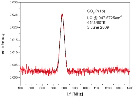
Still, even when assuming 5 MHz as linewidth of the local oscillator of THIS, this will lead only to a broadening of ∼310 kHz in the mea- surement of a FWHM = 40 MHz Venusian emission line (40 MHz is a lower limit, measured linewidths are usually around 45 MHz, see chapter 6.2.5, reducing the broadening effect of a noisy LO). This is well within the error bars of the temperature retrieval. As worst-case scenario with both lasers contributing equally to the 15 MHz broad- ening after two minutes of integration time, a FWHM of 10.6 MHz of the LO would result in an extra line broadening of 1.38 MHz re- sulting in an temperature error of ∼ 10 K.

Concluding this paragraph, I don’t assume the LO linewidth to broaden the measured non-LTE emission line significantly, but a fi- nal experiment to verify this assumption has to be done in the near future.

Figure 2.6: Direct heterodyne linewidth measurement of a cw QCL at 9.2 µm .

The QCL emission was fed as a signal into THIS. The emission was fitted with a

Gaussian. The calculated linewidth of 1.53 MHz reproduces the fluctuation band-

width of the spectrometer; therefore the laser linewidth is well below 1.53 MHz

[17].

(27)

2.1 Instruments: THIS 19

Laser stability

The spectral stability of the system was tested in the laboratory. To simulate observing conditions, a reference gas cell was observed for

∼ 1 second every 30 s for 75 minutes. The result is shown in Fig. 2.7.

The standard deviation of the spectral position of the QCL is 300 kHz. Long term deviations and concurrent line broadening can be ruled out due to the frequent measurements of the reference cell within the astronomical observation.

Figure 2.7: Stability measurement using a ethylene gas cell

2.1.3 The Detector

Currently a fast Mercury-Cadmium-Telluride (MCT) photo diode is implemented as mixer/detector in THIS. It is equipped with an op- tical resonant cavity in which the incident infrared radiation is re- flected several times. This enhances the absorption and thereby in- creases the quantum efficiency of the detector. To cover a wide spec- tral range, the chip contains four elements, each optimised for ad- jacent wavelength regions, enabling a coverage from 7.5 - ∼ 12 µ m . Quantum efficiencies of more than 80% are reached.

For the measurements at higher wavelengths, chapter 7, another

MCT detector without resonant cavity was used. There, I will also

go more into detail on MCT detectors in general.

(28)

Figure 2.8:

THIS set up at the observing table at the McMath-Pierce Solar Telescope, Kitt Peak. The spectrometer is the aluminium cube with the fading author above. On the right the corresponding electronics can be seen.

(29)

2.2 Instruments: IRHS / HIPWAC 21

2.2 Instruments: IRHS / HIPWAC

Infrared Heterodyne observations of planetary atmospheres already started in the 1970s with the detection of the non-LTE emission in the atmosphere of Mars. Since then, both planets, Venus and Mars were observed many times, mostly studied for winds and atmospheric composition. But much of the accumulated data was not analysed for temperatures. Within this work it was possible to re-analyse data taken in four observing runs from January 1990 until September 1991. Similar to both campaigns in March and April 2009 with THIS, Venus was observed shortly before and after inferior conjunction.

The first infrared heterodyne spectrometer (IRHS) was implemented in 1976 at the NASA Goddard Space Flight Center (GSFC) [19]. It was used at the Coudé foci of the McMath-Pierce Solar Telescope at Kitt Peak and the IRTF on Mauna Kea. When the Coudé room of the IRTF was decommissioned, a transportable version was built, the Heterodyne Instrument for Planetary Wind And Composition (HIP- WAC), being able to operate at the Cassegrain focus of the IRTF. The principle is of course the same as for THIS, in fact, both spectrom- eters make use of identical MCT detectors, but there are some big differences in the layout of both spectrometers.

The local oscillator

A CO

2

gas laser is the local oscillator of IRHS/HIPWAC. It is pos- sible to switch between two laser tubes which can be operated with different CO

2

isotopes and at various transitions to cover as much wavelength regions as possible. The desired transition can be se- lected by tilting an incorporated diffraction grating. The LO beam is also optically matched with the telescope beam before heterodyning.

The high output power of CO

2

lasers is an advantage compared to

early QCLs or lead salt diode lasers, it even makes attenuation nec-

essary, but the tuneablitiy is restricted to a small region around the

transition frequencies which can be realised by pressure and laser

cavity alignment variations. The laser frequency can be stabilised

using Lamb dip stabilisation (IRHS see below) or power peak stabil-

isation (HIPWAC) where the emission is locked to the peak of the

laser gain profile.

(30)

Lamb dip stabilisation Using Lamb dip stabilisation, the cen- tre frequency of the LO can be stabilised very precisely within

∼ 0.1 MHz [20]. This is realised by introducing a absorption cell into the laser cavity. Molecules in this cell will resonantly absorb radiation at the rest frequency of the laser transition (ν

lt

). In the case of IRHS, molecules then radiatively relax to the ground state by emitting a photon at 4.3 µm wavelength (which is the dominant de- excitation pathway compared to the 9.4 and 10.4 µm bands) which can be monitored. If the laser ν

lo

is detuned from ν

lt

, molecules can still absorb if their velocity along the cavity axis is Doppler shifting the laser photons from ν

_lo

to ν

_lt

in the molecule’s rest frame. This can be done in both axial directions. Shifting ν

_lo

towards ν

_lt

increases the 4.3 µ m emission as more molecules inhibit the right axial velocity.

At ν

_lo

= ν

_lt

only molecules with the axial velocity = 0 do absorb the radiation, leading to a dip in 4.3 µ m emission. Also, molecules being excited in the initial path leave fewer molecules to be excited in the return path of the cavity, which is further amplifying the dip.

Linewidth The initial laser gain width is dominated by the pressure broadening of 7.5 MHz/Torr for CO

2

yielding a ∼170 MHZ gain pro- file at ∼ 20 Torr gas pressure. The effective length of the laser cav- ity then selects the actual laser frequency which has a very narrow Lorentzian profile of less than 10 kHz FWHM for IRHS and basically the same value for HIPWAC.

Beam switching and Heterodyning

The switching between sky signal, sky reference can be done by us- ing the wobbling secondary mirror at the IRTF, which can be syn- chronised to the observing process of double beamswitch, or a by chopper wheel by which also a blackbody calibration source can be selected. The superpositioning of the signal radiation to the local oscillator is achieved by using a ZnSe beam splitter.

Back-end IF Analysis

The IF is analysed by two 64 channels RF filter banks. One low res-

olution filter bank with 25 MHz filter width providing a bandwidth

of 1.6 GHz. The high resolution (5 MHz, 320 MHz bandwidth) filter

(31)

2.2 Instruments: IRHS / HIPWAC 23

bank can be tuned within the low resolution bandwidth by mixing the IF with a radio frequency local oscillator. In this way narrow features like line peaks can be investigated using the high resolution filter bank, while broad features like the line wings are sufficiently resolved by the low resolution filter bank.

In recent years, HIPWAC also is starting to use an AOS back-end spectrometer and is currently evaluating QCLs as local oscillators due to the successful operation of both elements in THIS.

Figure 2.9: HIPWAC mounted at the Subaru telescope.

(32)

2.3 Expanding THIS to Longer Wavelengths

One main part of this thesis is the evaluation of mid-infrared detectors for THIS, with emphasis to longer wavelengths than 10 µ m . A detailed presentation of possible targets and laboratory measurements will be given in chapters 6 and 7. In this section, I will discuss the instrumental pros and cons, including a brief comparison to direct detection techniques.

Leaving the CO

2

region

Beyond 12 micron, there are many scientific targets which call for high spectral resolution, see chapter 6. THIS is currently starting to implement LOs with longer wavelengths, making it a unique in- strument in that wavelength region. There are molecules without permanent dipole moment like Acetylene which are not detectable at radio wavelengths or atomic lines like Magnesium (I) where in- vestigations of magnetic field induced Zeeman splitting makes high spectral resolution necessary. In contrast to HIPWAC which is re- stricted to narrow areas surrounding the CO

2

transitions, THIS can in principle cover any wavelength region, given the availability of QCLs.

2.3.1 Comparison: Heterodyning vs. Direct Detection

Infrared heterodyne spectroscopy fills a niche in contemporary as-

trophysical instrumentation. Usually, direct detection systems with

spectral resolutions of up to 10

⁵

are used for investigating astronom-

ical problems if high spectral resolution is needed. Direct detection

involves a dispersive element (usually a grating) and has obvious

advantages like not being limited by the quantum limit and by in-

strumental limits of the bandwidth. On the other hand, if extremely

high spectral resolution is needed (10

⁶

or higher) direct detection is

limited by the size of the necessary grating, which scales with the

product of wavelength and spectral resolution. At 10 µ m wave-

length and spectral resolution of 10

⁵

the necessary size of the grating

(which needs to be cryogenically cooled to reduce background noise)

is already 1 m and therefore on the limit of technical feasibility.

(33)

2.3 Expanding THIS to Longer Wavelengths 25

The quantum limit

Every heterodyne receiver adds noise to the observation. A conve- nient measure of this is the system temperature T

_sys

, an expression used in radio astronomy. It can be viewed as the transfer of all noise contributions of the receiver to an external source which then can be described by a brightness temperature a hypothetical, noise-free re- ceiver would see. The lower boundary of the system temperature is given by the so called ’quantum limit’:

T

_QL

=

^h·ν_k

B

It is the noise seen after the mixer of an ideal heterodyne receiver where all external noise contributions are zero.

In a real receiver, the system temperature is increased by the quan- tum efficiency η of the mixer non-perfect heterodyning, background IF photons, losses in the spectrometer optics etc. (all combined in the factor α ):

T

_Sys

= T

_QL

· (1 + α)

To experimentally determine the system temperature, usually the ’y- factor-method’ is used. The signals from two loads are compared to their known temperatures:

y =

_S^S^Hot

Cold

T

_sys

=

^J^Hot^−y·J_y−1^Cold

with: S

i

= observed output signals and J

i

= brightness Temperatures of the two loads. At 10 µm wavelength (T

QL

= 1440 K) system tem- peratures of less than 2500 K were measured with THIS, only about 70% above the quantum limit [1].

Sensitivity

A comparison of direct and heterodyne detection methods is a dif-

ficult task, because many different parameters have to be taken into

account and information given in the literature is usually not directly

comparable as different definitions are used. Here I try to compare

(34)

the values of the noise equivalent power (NEP, which depends on the frequency resolution) and show an estimation of the behaviour of the signal-to-noise ratio (SNR) with varying resolution and wave- length as discussed in detail in [21]. Generally, heterodyne detection suffers severely from the quantum limit at high frequencies, while direct detection is more affected by increasing background noise at longer wavelengths. If the contribution of the background exceeds the quantum limit, heterodyne systems perform better than direct detection because of the higher coupling efficiencies. This is spe- cially true if going to high resolutions where the throughput of di- rect detection instruments decreases. Frequency dilution effects even amplify the heterodyne advantage.

With the heterodyne system temperature one can calculate the NEP:

N EP = 2

³²

· k

_B

· T

_Sys

·

^q^δ^Res_q

, where δ

_Res

=

_L¹

max

R

L(ν) · dν is the resolution bandwidth, q is the ratio of fluctuation and resolution bandwidth q =

_δ^B^{F l}

Res

, B

_{F l}

=

⁽

RL(ν)·dν)²

RL²(ν)·dν

. L(ν) is the power transmission of the filter. q equals unity for a boxcar filter.

For example, the NEP for an ideal heterodyne receiver at 30 THZ is

N EP

_Ideal

= 7.9 · 10

⁻¹⁶

W/ √ Hz N EP

_{T HIS}

= 1.4 · 10

⁻¹⁵

W/ √

Hz

(with q = 1.5, λ = 10 µm T

_Ideal

= T

_QL

= 1440K, T

_{T HIS}

= 2500K and δ

_Res

= 300M Hz).

The NEP for TEXES (Texas Echelon Cross Echelle Spectrograph [22]) is given by:

N EP

_{T exes}

= 3.9 · 10

⁻¹⁶

W/ √ Hz

(for 1.5 m telescope radius, λ = 10 µ m , 300 MHz resolution)

This corresponds to a noise temperature of ∼ 700 K, or 50% of the heterodyne quantum limit.

With such spectral resolution, the NEP of TEXES is lower by a fac-

tor of 3.5 meaning THIS needs 12 times the observing time to get

(35)

2.3 Expanding THIS to Longer Wavelengths 27

the same SNR. However, at a higher spectral resolution of 10 MHz the NEP of THIS reduces to N EP

_{T HIS}

= 2.5 · 10

⁻¹⁶

W/ √

Hz , whereas TEXES is suffering from frequency dilution. At this resolution het- erodyne spectroscopy is clearly advantageous to direct detection.

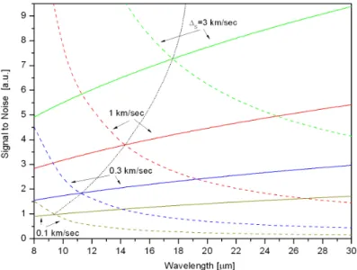
In order to achieve an illustrative comparison of the sensitivities of

THIS and TEXES, [21] generated a plot showing the change of the

signal to noise ratio with wavelength and frequency resolution, see

Fig. 2.10. The plot is based on the best case sensitivity values found

in the literature for TEXES [22] and THIS [23] which are interpolated

to longer wavelengths. Plotted is the achievable SNR over observed

wavelength for a given signal width in km/s (the frequency width of

the smallest feature to be detected). It can be seen that the sensitiv-

ity of the heterodyne system rises with increasing wavelength due

to the decrease of the quantum limit. Direct detection on the other

hand shows a decreasing sensitivity towards longer wavelengths as

the background contribution increases and the frequency dilution

becomes more important. This is the explanation for the existence

of a turnover point for every signal width where one technique be-

comes more advantageous than the other. The dotted line shows this

border for TEXES and THIS. TEXES is more sensitive at short wave-

lengths and at lower resolution, whereas THIS is preferred at long

wavelengths and at high spectral resolution.

(36)

Figure 2.10: Direct (dotted) vs heterodyne (solid) signal-to-noise ratios for dif-

ferent signal widths.

(37)

Chapter 3

Venus Atmosphere

Venus, Earth’s neighbour planet, is (apart from the moon) the brightest object in the night sky. It was targeted by Galileo Galilei’s first telescope, and today it is again target of modern science being observed from the ground as well as from space with current and future orbiters like ESA’s Venus Express and the Japanese orbiter Akatsuki.

The atmosphere of Venus consists of ∼96% CO

2

and ∼3% N

2

, similar to Mars. In the very contrast to Mars, the density is extremely high, reaching 92 bar at the surface (Mars: ∼6 mbar). Venus also shows similarities to Earth as the diameter is comparable, but most features are drastically different. Its spin direction is contrary to the rotation around the sun, and it rotates extremely slow. In fact, one sidereal day is longer than a sidereal year, only the ’wrong’ direction of rotation leads to a ’shorter’ (166 Earth days) solar day. This very long exposure to the sun together with a greenhouse-heated CO

2

atmosphere leads to a completely different atmospheric picture compared to that of Earth.

Nevertheless, the physics is the same on every planet. Refined atmo- spheric models, developed from data collected by countless satellites and weather stations on Earth, able to predict the weather for some days and the climatic changes for decades, should in principle be applicable to all other planetary atmospheres, given that the differ- ent initial conditions like composition and solar flux are taken into account properly. In reverse, lessons learnt on the Venusian atmo- sphere can improve the understanding of climatological procedures

29

(38)

on Earth. Apart from scientific curiosity, this is the main motiva- tion for observing planetary atmospheres. While refined global cir- culation models (GCMs) exist for Mars (extensively studied by nu- merous landers, orbiters and ground-based facilities) and Titan (the biggest moon of Saturn, possessing a dense atmosphere which is very ’earth-like’), models for the Venusian atmosphere were rather simple until the arrival of Venus Express, which relaunched the sci- entific interest in Venus and lead to many surprises and open ques- tions.

Temperatures are a key parameter in the understanding of atmo- spheric structure, dynamics and composition. Strong temperature gradients due to the long solar exposure drive global patterns like the subsolar to antisolar stream in the upper atmosphere. Chemical processes are dependent on the temperature and changes of some 10 K can lead to fundamental changes in reaction chains.

In the following chapter, I will introduce shortly the current knowl- edge about Venus’ atmosphere, summarise the main observation campaigns measuring mesospheric temperatures and will discuss the non-LTE emission of CO

2

, which enables infrared heterodyne temperature measurements.

3.1 Venus Atmosphere: Models

The atmosphere of Venus is dominated by two fundamentally different regions. One region is the dense cloud layer in the tro- posphere from ∼ 40 km to ∼ 60 km altitude, covering the whole planet and rotating up to 60 times faster than the planet itself. This massive ’superrotation’ is still not understood today. The other dominating dynamical feature is the sub-solar to anti-solar (SSAS) flow, located in the thermosphere above ∼ 140 km. It can be seen as a global anticyclone(SS)/cyclone(AS) system, driving a spherically symmetric wind from the subsolar point towards the antisolar point (see also Fig.3.1).

These two dynamical features of course have fundamental influence

on the temperature field. In the troposphere, within the superro-

tation, the atmosphere is turbulent, well mixed and temperatures

do not change between day and nightside. Due to the CO

2

atmo-

sphere and the dense cloud layers, temperatures at the surface are

greenhouse-driven and reach up to ∼ 750 K, and almost constantly

cool down to about 230 K at the cloud tops at 60 km altitude.

(39)

3.1 Venus Atmosphere: Models 31

Figure 3.1: Modelled thermospheric temperatures (colours) and subsequent sub- solar to anti-solar flow (arrows) in 180 km altitude [24].

In the SSAS dominated region, there are huge diurnal temperature differences up to ∼ 200 K

¹

. At the dayside, there is an inversion and temperatures again reach more than 300 K at altitudes above 180 km.

Vice versa, at night temperatures cool to ∼ 120 K. This diurnal differ- ence starts to become significant above ∼ 100 km.

Infrared heterodyne spectroscopy is targeting the transition zone be- tween superrotation and SSAS flow at around 115 km altitude. Of course, it is interesting to see how both regions interact and maybe how sharp the transition is, as this will be valuable information con- straining evolving global circulation models.

Models of the atmosphere of Venus have been very simple until the arrival of Venus Express because of the lack of sufficient data. Since the first probes like Venera 1 (which was actually the first spacecraft reaching another planet) and Mariner 2 in 1961/62, Pioneer Venus was the only space mission dedicated to investigate the atmosphere of Venus. It consisted of several landers and the Pioneer Venus Or- biter (PVO) which stayed in orbit from 1978 until 1992. Together

1This was leading to the differentiation of the dayside ’thermosphere’ and the nightside

’cryosphere’. For simplicity, and as all infrared heterodyne measurements are dayside only, I will describe altitudes higher than∼120 km as ’thermosphere’.

(40)

with a series of Venera landers and orbiters it provided first detailed insight which resulted in the empirical ’Venus International Refer- ence Atmosphere’ (VIRA) model. Today, there are various attempts to update the VIRA model and also to derive complete global circu- lation models.

Venus International Reference Atmosphere (VIRA)

VIRA, published in 1985 [25] is based on data accumulated during the Pioneer-Venus mission and numerous Venera probes. After the historic first interplanetary probe Venera 1 (1961) the climax of these observations was in the late 1970s with the arrival of Pioneer-Venus 1 and 2. With data from orbiters and Landers the first detailed picture of another planet emerged. It was updated in 1997 (VIRA-2 [26], with further additions 2006 and 2007 [27, 28]) after the end of PVO and after more data was acquired e.g. from the Magellan, Galileo, Venera and VEGA missions.

The observed data and an averaged temperature profile [29] can be seen in Fig. 3.2. In the altitude region important for this thesis, there is only very few data from all VIRA contributing instruments. With three descent probes, one at the day side, one at the night side (both in mid- latitudes) and one in the north polar region, conclusions to the general atmosphere can only be drawn if the atmosphere is glob- ally stable and homogeneous. This is already challenged by the high variability of the measured temperatures during the descent of the day side probe above 110 km.

Resulting from this lack of data, the spatial resolution is rather broad

with a latitudinal separation of up to 30 degrees. It therefore can only

be handled as a very averaged global model which ignores possible

local or temporal variations. Since the first view of the upper atmo-

sphere described it as rather static and uniform, VIRA was a suit-

able model in the beginning, but today more and more deviations

are observed (see section 3.2 below). However, despite its known

problems, VIRA is still the most used reference for atmospheric tem-

peratures.

(41)

3.1 Venus Atmosphere: Models 33

Figure 3.2:

Temperature Profiles taken with Pioneer Venus and Venera probes [25]. As indicated, Pioneer Venus 2 deployed three probes into the Venusian atmosphere, one on the day side one on the night side and one in the north polar region. The inset shows the averaged VIRA model [29], which clearly under-represents the dayside variations seen above 110 km.

(42)

Modern global circulation models (GCM)

Recently, there are many attempts to create a more realistic model for the atmosphere of Venus. However, they all are either still in an early phase of evolution or restricted to distinct atmospheric re- gions. For example the Venus Thermosphere GCM by Bougher et al.(VTGCM [30, 31]) was developed from Earth GCMs [32]. It mod- els nicely the SS-AS flow but is restricted to altitudes higher than 100 km. For the middle atmosphere (30-90 km altitude) there is a lot of data from Venus Express. To couple this observationally good cov- ered region to the thermosphere is the goal of the model developed at the Imperial College by Mueller-Wodarg and coworkers. They are trying to adapt a model of Titan’s atmosphere [33] to Venus. Ti- tan has a more ’earth-like’ atmosphere, which makes it easier to pre- dict using well-proven models of the Earth’s atmosphere. Assuming boundary conditions for the cloud tops and the high thermosphere, this model is targeted at the mesosphere of Venus with a quite empir- ical approach, trying to incorporate results of observations as soon as possible.

In contrast, Lebonnois et al. ([34]) is starting from an analytical point of view, at first trying to reproduce the very basic attributes of Venus atmosphere like the superrotation from basic physical con- siderations and only in a second step to adapt the model to specific observations.

3.2 Ground-based Observations

Despite the increasing interest in Venus and its atmosphere since the arrival of Venus Express, temperature measurements in the meso- sphere are still insufficient. The temperatures presented in this the- sis are the only ones at the day side of Venus probing the upper mesosphere with an adequate spatial resolution. In this chapter I will summarise other measurements in the vicinity and discuss their comparability to the infrared heterodyne results.

Ground based observations are mostly done using sub-mm obser- vations of CO. I will here present measurements by Clancy et al.

and Rengel et al., as they will be later compared to infrared het-

erodyne measurements. Other methods include observations of air-

glow emission of molecular oxygen at 1.3 µ m , but as they are pure

(43)

3.2 Ground-based Observations 35

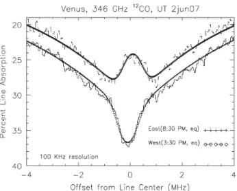
Figure 3.3: Observed

¹²

CO absorption line at 346 GHz (J=2 7→ 3), from Clancy et al. [35]. From fits to the line shape, temperature profiles can be modelled.

nightside observations they are mentioned here more to get a gen- eral idea about temperature measurements in the upper atmosphere of Venus.

3.2.1 Sub-mm

Sub-mm measurements of CO absorption lines (see Fig. 3.3) of various isotopes and at different rotational transitions provide temperature profiles from 75–110 km altitude. Fig. 3.4 shows the diurnal temperature difference which is clearly visible in the line centre. While the cold night side produces an enhanced dip, on day side observations even a little (LTE) emission is visible.

To derive the temperature profile from the measured line-shape, one

has to include the CO mixing profile and an a-priori temperature

profile as a starting point for fit algorithms. CO mixing profiles can

be retrieved from simultaneously fitting different spectra constrain-

ing different altitude ranges (e.g.

¹²

CO and

¹³

CO, [35]). As a-priori

temperature profile, usually the VIRA model is used [36]. When

(44)

fitting the temperature profile, constant atmospheric spheres are assumed [36].

A major drawback of ground based sub-mm observations of plane- tary atmospheres is the low spatial resolution due to the big field of view. Using the James Clerk Maxwell Telescope (JCMT, Mauna Kea, Hawaii, 15 m dish) and a CO transition line at 346 GHz, the resulting FWHM of the antenna beam is 14 arc-seconds (valid for most Clancy et al. observations). This is more than 8 times larger than THIS at the McMath-Pierce Solar Telescope (FOV: 1.7 arc-seconds) or even 16 times larger than THIS or HIPWAC at the IRTF (FOV: 0.85 arc- seconds) . As an example, at Venus’s maximum elongation (∼50%

illumination) the sub-mm beam fills the whole day side, whereas in- frared heterodyne can do many independent measurements all over the illuminated disk.

This has also to be taken into account when thinking about the sub- mm temperature profile modelling, assuming constant spheres. Re- solving large fraction of a planetary disc, this can be only an approx- imation.

Summarising, sub-mm observations of CO are a nice tool to obtain mesospheric temperature profiles at both, day and nightside of a planet, but they lack spatial resolution which prevents detailed infor- mation which can be provided by infrared heterodyne spectroscopy (at the dayside and at the emission altitude).

Clancy et al.

One of the most thorough ground based studies of upper atmo- spheric temperatures has been done by Clancy et al. using mm (1982,

’85, ’86, ’88, and ’90 using the Kitt Peak NRAO–12 m millimeter ob-

servatory) and sub-mm (1999, 2000, ’01, ’02, ’07 and ’09 using the

JCMT) observations of carbon monoxide (CO). Observations were

carried out from the mid eighties until today. Being able to observe

both,day and night sides of Venus and probing altitudes from 75 to

100 km, these are valuable data to compare to infrared heterodyne

measurements. Temperatures observed tend to be higher than ex-

pected from VIRA, detailed profiles are discussed in chapter 4.

(45)

3.2 Ground-based Observations 37

Figure 3.4: Centres of the line displayed in Fig. 3.3, for both day (West) and night side (East). Big diurnal temperature variations are evident (night side dip vs. day side emission) as well as different wind induced Doppler shifts.

Rengel et al.

Rengel et al. [36, 37] observed also CO but J=2 7→ 1 transitions at 220 and 230 GHz. Using the 10 m Heinrich Hertz Submillimeter Telescope (HHSMT, Mt. Graham, Arizona) their FOV was ∼ 33 arc- seconds with the apparent diameter of Venus of 24 arc-seconds dur- ing the observations. The observed temperatures in principle agree with VIRA data, but do show big variability (see Fig. 3.5). Taken within 24 hours, 3 out of 4 observations agree within the error bars.

One observation (red, Fig. 3.5) shows significant deviations. These

variations partly might originate from pointing errors as some night-

time features of the thermal profile appear also in this daytime mea-

surements. The warm layer at 105 km altitude is seen very promi-

nently in every nighttime profile. Also the inversion layer at 70 km

is seen in other nighttime profiles. However, using the above men-

tioned beam sizes, they had to point off the planet anyway to receive

only the signal from the selected hemisphere. Usual pointing errors

in the order of an arc-second should be negligible. This would be

another indication for a high intrinsic variability of the Venus atmo-

sphere.

(46)

Figure 3.5: Superposition of four dayside observations of

¹²

CO(J=2 7→ 1) at 230 GHz from [37]. Dashed line: VIRA profile. Temperature variations reach up to 50 K within 24 hours.

3.2.2 Air-glow Measurements

Air-glow emission is the result of recombination of oxygen atoms

which are formed by photo-dissociation of CO

2

molecules on the

day side of Venus. These atoms are carried by the SSAS flow to the

night side, descend to higher density regions, recombine producing

excited O

2

which then emits the air-glow photons. Temperatures

can be retrieved by fitting the rotational temperature to the relative

strengths of individual lines of the emitting band [38]. Observations

were taken at the Anglo-Australian Telescope using an infrared im-

ager and spectrograph at 1.3 µm wavelength and with a spectral res-

olution of 2400 ( λ/δλ ). Results show mean temperatures of around

190 ± 10 K in agreement to earlier measurements [39, 40]. These

temperatures are significantly higher (15-30 K) than those expected

from VIRA see Fig. 3.6. The altitude of the air-glow emission can be

constrained by chemical model predictions to 90-100 km, validated

(47)

3.2 Ground-based Observations 39

by Venus Express data described in the following section.

Figure 3.6: Nighttime temperatures from O

2

Observations of Upper Mesosphere Temperatures on Venus and Evaluation of Mid-Infrared Detectors for the Tuneable Heterodyne Infrared Spectrometer (THIS)