Testing the parametric form of the volatility in continuous time diffusion models - an empirical process approach
Holger Dette Ruhr-Universit¨at Bochum
Fakult¨at f¨ur Mathematik 44780 Bochum, Germany e-mail: holger.dette@rub.de
FAX: +49 234 3214 559
Mark Podolskij Ruhr-Universit¨at Bochum
Fakult¨at f¨ur Mathematik 44780 Bochum, Germany e-mail: podolski@cityweb.de
November 18, 2005
Abstract
In this paper we present two new tests for the parametric form of the variance function in diffusion processes dXt =b(t, Xt) +σ(t, Xt)dWt.Our approach is based on two stochastic processes of the integrated volatility. We prove weak convergence of these processes to centered processes whose conditional distributions given the process (Xt)t∈[0,1]are Gaussian.
In the special case of testing for a constant volatility the limiting process is the standard Brownian bridge in both cases. As a consequence an asymptotic distribution free test (for the problem of testing for homoscedasticity) and bootstrap tests (for the problem of testing for a general parametric form) can easily be implemented. It is demonstrated that the new tests are more powerful with respect to Pitman alternatives than the currently available procedures for this problem. The asymptotic advantages of the new approach are also observed for realistic sample sizes in a simulation study, where the finite sample properties of a Kolmogorov- Smirnov test are investigated.
Keywords and Phrases: Specification tests, integrated volatility, bootstrap, heteroscedasticity, stable convergence, Brownian Bridge
1 Introduction
Modeling the dynamics of interest rates, stock prices exchange rates is an important problem in mathematical finance and since the seminar papers of Black and Scholes (1973) and Merton (1973) many theoretical models have been developed for this purpose. Most of these models are continu- ous time stochastic processes, because information arrives at financial markets in continuous time [see Merton (1990)]. A commonly used class of processes in mathematical finance for representing
asset prices are Itˆo diffusions defined as a solution of the stochastic differential equation dXt =b(t, Xt)dt+σ(t, Xt)dWt
(1.1)
where (Wt)t is a standard Brownian motion and b and σ denote the drift and volatility, respec- tively. Various models have been proposed in the literature for the different types of options [see e.g. Black and Scholes (1973), Vasicek (1977), Cox, Ingersoll and Ross (1985), Karatzas (1988), Constantinides (1992) or Duffie and Harrison (1993) among many others]. For a reasonable pricing of derivative assets in the context of such models a correct specification of the volatility is required and good estimates of this quantity are needed. For example, the pricing of European call options crucially depends on the functional form of the volatility [see Black and Scholes (1973)] and the same is true for other types of options [see e.g. Duffie and Harrison (1993) or Karatzas (1988) among many others].
A (correct) specification of a parametric form for the volatility has the advantage that the problem of its estimation is reduced to the determination of a low dimensional parameter. On the other hand a misspecification of drift or variance in the diffusion model (1.1) may lead to an inadequate data analysis and to serious errors in the pricing of derivative assets. Therefore several authors propose to check the postulated model by means of a goodness-of-fit test [see Ait Sahalia (1996), Corradi and White (1999), Dette and von Lieres und Wilkau (2003)]. Ait Sahalia (1996) assumes a time span approaching infinity as the sample size increases and considers the problem of testing a joint parametric specification of drift and variance, while in the other references a fixed time span is considered, where the discrete sampling interval approaches zero, and a parametric hypothesis regarding the volatility function is tested. This modeling might be more appropriate for high frequency data.
In the present paper we also consider the case of discretely observed data on a fixed time span, say [0,1], from the model (1.1) with increasing sample size. As pointed out by Corradi and White (1999) this model is appropriate for analyzing the pricing of European, American or Asian options. These authors consider the sum of the squared differences between a nonparametric and a parametric estimate of the variance function at a fixed number of points in the interval [0,1].
Although this approach is attractive because of its simplicity, it has been argued by Dette and von Lieres und Wilkau (2003) that the results of the test may depend on the number and location of the points, where the parametric and nonparametric estimates are compared. Therefore these authors suggest a new test for the parametric form of the volatility in the diffusion model (1.1), which does not depend on the state x, i.e. σ(t, Xt) =σ(t). The test is based on an L2-distance between the volatility function in the model under the null hypothesis and alternative. This approach yields a consistent procedure against any (fixed) alternative, which can detect local alternatives converging to the null hypothesis at a rate n−1/4. In the present paper an alternative test for the parametric form of the volatility function is proposed, which is based on an empirical process of the integrated volatility. Our motivation for considering functionals of stochastic processes as test statistics stems from the fact that tests of this type are more sensitive with respect to Pitman alternatives. Moreover the new tests are also applicable for testing parametric hypotheses on the volatility, which which depend on the state x.
In Section 2 we introduce some basic terminology and describe two kinds of parametric hypothe- ses for the volatility function. We also define two types of stochastic processes of the integrated volatility, which will be used for the construction of test statistics for these hypotheses. Section
3 contains our main results. We show convergence in probability of the stochastic processes to a random variable, which vanishes if and only if the null hypothesis is satisfied. Moreover, we also establish weak convergence of appropriately scaled processes of the integrated volatility to a centered process under the null hypothesis of a parametric form of the volatility. Consequently, the Kolmogorov-Smirnov and Cram´er von Mises functional of these processes are natural test sta- tistics. In general the limiting process is a complicated “function” of the data generating diffusion, but conditioned on the diffusion (Xt)t∈[0,1] it is a Gaussian process. In the problem of testing for homoscedasticity these tests are asymptotically distribution free and the limit distribution is given by a Brownian bridge. In Section 4 we study the finite sample properties of the proposed method- ology and compare the new procedure with the currently available tests for the parametric form of the volatility function. For high frequency data the new tests yield a reliable approximation of the nominal level and substantial improvements with respect to power compared to the currently available procedures. Finally, all proofs and some auxiliary results are presented in an appendix.
2 Specification of a parametric form of the volatility
Let (Wt)t≥0 denote a standard Brownian motion defined on an appropriate probability space (Ω,F,(Ft)0≤t≤1, P) with corresponding filtration FtW = σ(Ws,0 ≤ s ≤ t) and assume that the drift and variance function in the stochastic differential equation (1.1)
b : [0,1]×R→R σ : [0,1]×R→R
are locally Lipschitz continuous, i.e. for every integerM > 0 there exists a constantKM such that
|b(t, x)−b(t, y)|+|σ(t, x)−σ(t, y)| ≤KM |x−y| (2.1)
for all t ∈[0,1], x, y ∈[−M, M], and there exists a constantK such that
|b(t, x)|2+|σ(t, x)|2 ≤K2(1 +|x|2) (2.2)
for all t ∈ [0,1], x ∈ R. It is well known that for an F0-measurable square integrable random variable ξ, which is independent of the Brownian motion (Wt)t∈[0,1], the assumptions (2.1) and (2.2) admit a unique strong solution (Xt)t∈[0,1] of the stochastic differential equation (1.1) with initial condition X0 =ξ which is adapted to the filtration (Ft)0≤t≤1 [see e.g. Karatzas and Shreve (1991) p. 289]. The solution of the differential equation can be represented as
Xt =ξ+ Z t
0
b(s, Xs)ds+ Z t
0
σ(s, Xs)dWs a.s., (2.3)
where Xt is Ft-measurable for all t ∈ [0,1] and the paths t → Xt are almost surely continuous.
In the literature various parametric functions have been proposed for different types of options [see e.g. Black and Scholes (1973), Vasicek (1977), Cox, Ingersoll and Ross (1985), Karatzas (1988), Constantinides (1992) or Duffie and Harrison (1993) among many others]. In principle the assumption on the volatility function in these models can be formulated in two ways that is
H¯0 :σ2(t, Xt) =
d
X
j=1
θ¯jσ¯j2(t, Xt) ∀ t∈[0,1] (a.s.) , (2.4)
or
H0 :σ(t, Xt) =
d
X
j=1
θjσj(t, Xt) ∀ t∈[0,1] (a.s.) , (2.5)
where ¯σ12, . . . ,σ¯d2,respectivelyσ1, . . . , σdare given and known volatility functions and ¯θ = (¯θ1, . . . ,θ¯d), θ = (θ1, . . . , θd)∈Θ⊂Rd are unknown finite dimensional parameters. Throughout this paper we assume additionally that the drift and variance function satisfy a further Lipschitz condition of order γ > 12,i.e.
|b(t, x)−b(s, x)|+|σ(t, x)−σ(s, x)| ≤L|t−s|γ (2.6)
|b(t, x)−b(s, x)|+|σj(t, x)−σj(s, x)| ≤L|t−s|γ , j = 1, . . . , d,
for all s, t ∈[0,1], L > 0. Note that the hypothesis (2.4) refers to the variance function σ2 while the formulation (2.5) directly refers to the factor of the term dWs in the stochastic differential equation (1.1). There exist in fact many models for prices of financial assets traded in continuous time, where both hypotheses are equivalent [see e.g. Vasicek (1977), Cox, Ingersoll and Ross (1985), Brennan and Schwartz (1979), Courtadon (1982), Chan, Karolyi, Longstaff and Sanders (1992)], but in general these hypotheses are not equivalent. A typical example for such a case is given by
H¯0 : σ2(t, Xt) = ¯ϑ1+ ¯ϑ2X12, (a.s.) (2.7)
H0 : σ(t, Xt) =ϑ1+ϑ2|Xt|, (a.s.) (2.8)
which is a slight generalization of the models considered in the cited references. We begin our discussion with the construction of a test statistic for the hypothesisH0in (2.5) and since the law of the processX depends only onσ2 [see Revuz and Yor (1999) p. 293] we assume that the functions σ, σ1, . . . , σd are strictly positive and linearly independent on every compact set [0,1]×[a, b],a < b.
We assume additionally that σ : [0,1]×R→ R is twice continuously differentiable such that for some constant F >0
sup
s,t∈[0,1]
E[( ∂
∂yσ(s, Xt))4]< F, sup
s,t∈[0,1]
E[( ∂2
∂y2σ(s, Xt))4]< F (2.9)
and
sup
s,t∈[0,1]
E[( ∂
∂y{σi(s, Xt)σj(s, Xt)})4]< F, sup
s,t∈[0,1]
E[( ∂2
∂y2{σi(s, Xt)σj(s, Xt)})4]< F (2.10)
for all 1 ≤i, j ≤d, where the differentiation in (2.9) and (2.10) is performed with respect to the second argument. Throughout this paper we assume that
E[|ξ|4]<∞, (2.11)
and that the functions σ1, . . . , σd in the linear hypothesis (2.5) satisfy the same assumptions (2.1), (2.2) and (2.9) as the volatility function σ. For the discussion of hypothesis (2.4) we need to replace σ by σ2 in assumption (2.9), σi by ¯σi2 in (2.10) and 4 by 8 in assumption (2.11).
For testing the hypothesis (2.5) we consider the following stochastic process Mt :=
Z t 0
nσ(s, Xs)−
d
X
j=1
θminj σj(s, Xs)o ds , (2.12)
where the vector θmin = (θmin1 , . . . , θdmin)T is defined by θmin := argminθ∈Rd
Z 1 0
nσ(s, Xs)−
d
X
j=1
θjσj(s, Xs)o2
ds . (2.13)
Note that the null hypothesis in (2.5) is satisfied if and only if Mt = 0 ∀ t∈[0,1] a.s.
(2.14)
and that we use an L2-distance to determine the best approximation of σ by linear combination of the functions σ1, . . . , σd. This choice is mainly motivated by the sake of transparency and other distances as the L1-distance could be used as well with an additional amount of technical difficulties.
From standard Hilbert space theory [see Achieser (1956)] we obtain θmin =D−1C ,
(2.15)
where the matrix D= (Dij)1≤i,j≤d and the vector C = (C1, . . . , Cd)T are defined by Dij := hσi, σji2,
(2.16)
Ci := hσ, σii2, (2.17)
and h·,·i2 denotes the standard inner product for functions f, g : [0,1]×R→R, that is hf, gi2 =
Z 1 0
f(t, Xt)g(t, Xt)dt (2.18)
(here and throughout this paper we assume that the integrals exist almost surely, whenever they appear in the text). Throughout this paper we also assume the existence of the expectation
E[det(D)−ρ]<∞ (2.19)
for some ρ >0. The quantities in (2.16) and (2.17) can easily be estimated by Dˆij := 1
n
n
X
k=1
σi(k n, Xk
n)σj(k n, Xk
n)−→P Dij, (2.20)
Cˆi := µ−11n−12
n
X
k=1
σi(k−1 n , Xk−1
n )|Xk
n −Xk−1
n |−→P Ci , (2.21)
where the symbol −→P means convergence in probability and µ1 is the first absolute moment of a standard normal distribution. With the notation
Dˆ = ( ˆDij)1≤i,j≤d, (2.22)
Cˆ = ( ˆC1, . . . ,Cˆd)T (2.23)
we obtain
θˆmin := ˆD−1Cˆ (2.24)
as estimate for the random variable θmin. We finally introduce the stochastic process Mˆt := ˆBt0−BˆtTDˆ−1C ,ˆ
(2.25)
as estimate of the process (Mt)t∈[0,1]defined in (2.12), where the quantities ˆBt0and ˆBt = ( ˆBt1, . . . ,Bˆtd)T are given by
Bˆt0 := µ−11n−12
bntc
X
k=1
|Xk
n −Xk−1 n |, (2.26)
Bˆti := 1 n
bntc
X
k=1
σi(k n, Xk
n), 1≤i≤d, (2.27)
respectively. Note that Mt = 0 (a.s.) for all t ∈ [0,1] if and only if the null hypothesis H0 is satisfied. Consequently, it is intuitively clear that the rejection of the null hypothesis for large values of
sup
t∈[0,1]|Mˆt| , Z 1
0 |Mˆt|dt or Z 1
0 |Mˆt|2dt yields a consistent test for the above problem.
Before we make these arguments more rigorous we briefly present the corresponding testing pro- cedure for the hypothesis (2.4). In this case the analogue of the stochastic process Mt is defined by
Nt :=
Z t 0
nσ2(s, Xs)−
d
X
j=1
θ¯jminσ¯j2(s, Xs)o ds , (2.28)
where the random variable ¯θmin = (¯θmin1 , . . . ,θ¯mind )T is given by θ¯min := argminθ¯∈Rd
Z 1 0
nσ2(s, Xs)−
d
X
j=1
θ¯jσ¯2j(s, Xs)o2
ds . (2.29)
The nonobservable stochastic process can easily be estimated from the available data by Nˆt := ¯Bt0−B¯tTD¯−1C ,¯
(2.30) where
D¯ij := 1 n
n
X
k=1
¯ σi2(k
n, Xk
n)¯σj2(k n, Xk
n), i, j = 1, . . . , d (2.31)
C¯i :=
n
X
k=2
¯
σi2(k−1 n , Xk−1
n )|Xk
n −Xk−1
n |2, i= 1, . . . , d (2.32)
and the quantities ¯Bt0 and ¯Bt = ( ¯Bt1, . . .B¯td)T are given by B¯t0 :=
bntc
X
k=1
|Xk
n −Xk−1 n |2, (2.33)
B¯ti := 1 n
bntc
X
k=1
¯ σi2(k
n, Xk
n), 1≤i≤d.
(2.34)
In the following section we investigate the stochastic properties of the processes (√
n( ˆMt−Mt))t∈[0,1]
and
(√
n( ˆNt−Nt))t∈[0,1].
In particular, we will prove weak convergence of these processes to centered processes, which are conditioned on the process (Xt)t∈[0,1] Gaussian processes. This is the basic result for the application of these processes in the problem of testing for the parametric form of the volatility in a continuous time diffusion model. The reason for considering both processes is twofold. On the one hand the weak convergence of the process √
n( ˆMt−Mt) can be established under weaker assumptions on the model (1.1). On the other hand the statistic √
n( ˆNt − Nt) can easily be extended to vector-valued diffusions [see Remark 3.7].
3 Main results
For the sake of brevity we mainly restrict ourselves to a detailed derivation of the stochastic properties of the process ˆMt. The corresponding results for the process ˆNt can be obtained by similar arguments and the main statements are given at the end of this section for the sake of completeness. We begin our discussion with two auxiliary results regarding the estimators ˆD and Bˆti defined in (2.22) and (2.27), which are also of own interest. Throughout this paper µi denotes the ith absolute moment of a standard normal distribution (i= 1,2). Our first results clarify the order of difference between the empirical quantities ˆCi, ˆBti, ˆDij and their theoretical counterparts Ci, Bti,Dij, respectively.
Lemma 3.1. If the assumptions stated in Section 2 are satisfied we have Bˆti−
Z t 0
σi(s, Xs)ds =op(n−12) 1≤i≤d Dˆ −D=op(n−12)
Throughout this paper the symbol
Xn Dst
−→X
means that the sequence of random variables converges stably in law. Recall that a sequence of d-dimensional random variables (Xn)n∈N converges stably in law with limit X, defined on an appropriate extension (Ω0,F0, P0) of a probability space (Ω,F, P), if and only if for any F- measurable and bounded random variable Y and any bounded and continuous function g the convergence
nlim→∞E[Y g(Xn)] = E[Y g(X)]
holds. This is obviously a slightly stronger mode of convergence than convergence in law [see Renyi (1963), Aldous and Eagleson (1978) for more details on stable convergence]. The following Lemma shows that the random variables ˆBt0 and ˆCi defined in (2.26) and (2.23) converge stably in law if they are appropriately normalized.
Lemma 3.2. If the assumptions stated in Section 2 are satisfied we have for anyt1, . . . , tk ∈[0,1]
√n
Bˆt01−< σ,1>t21 ...
Bˆt0k−< σ,1>t2k Cˆ1−C1
...
Cˆd−Cd
Dst
−→ µ−11 q
µ2−µ21 Z 1
0
Σ
1 2
t1,...tk(s, Xs) dWs0 ,
where W0 denotes a (d+k)-dimensional Brownian motion, which is independent of theσ-fieldF, and the matrix Σt1,...tk(s, Xs) is defined by
Σt1,...tk(s, Xs) =
v11(s, Xs) · · · v1k(s, Xs) w11(s, Xs) · · · w1d(s, Xs)
... . .. ... ... . .. ...
vk1(s, Xs) · · · vkk(s, Xs) wk1(s, Xs) · · · wkd(s, Xs) w11(s, Xs) · · · wk1(s, Xs) s11(s, Xs) · · · s1d(s, Xs)
... . .. ... ... . .. ...
w1d(s, Xs) · · · wkd(s, Xs) sd1(s, Xs) · · · sdd(s, Xs)
(3.1)
with
vij(s, Xs) = σ2(s, Xs)1[0,ti∧tj)(s) 1≤i≤k
wij(s, Xs) = σj(s, Xs)σ2(s, Xs)1[0,ti)(s) 1≤i≤k , 1≤j ≤d sij(s, Xs) = σi(s, Xs)σj(s, Xs)σ2(s, Xs) 1≤i, j ≤d
and
< σ,1>t2= Z t
0
σ(s, Xs)ds.
Note that the matrix Σt1,...tk(s, Xs) defined in (3.1) can be represented as Σ1/2t1,...,tk(s, Xs) = gt1,...,tk(s, Xs)gt1,...,tk(s, Xs)T
pgt1,...,tk(s, Xs)Tgt1,...,tk(s, Xs), (3.2)
where the vector gt1,...,tk(s, Xs) is defined by
gt1,...,tk(s, Xs) = (σ(s, Xs)I[0,t1)(s), . . . , σ(s, Xs)I[0,tk)(s), (3.3)
σ1(s, Xs)σ(s, Xs), . . . , σd(s, Xs)σ(s, Xs))T. Now we state one of our main results. For this purpose we define the process
An(t) =√
n( ˆMt−Mt) (t∈[0,1]) (3.4)
and obtain the following result.
Theorem 3.3. If the assumptions given in Section 2 are satisfied, then the process (An(t))t∈[0,1]
defined in (3.4) converges weakly onD[0,1]to a process(A(t))t∈[0,1], which is Gaussian conditioned on the σ-fieldF. Moreover, the finite dimensional conditional distributions of the limiting process (A(t1), . . . A(tk))T are uniquely determined by the conditional covariance matrix
µ−12(µ2−µ21) V Z 1
0
Σt1,...tk(s, Xs) ds VT , (3.5)
where the k×(d+k)-dimensional matrix V is defined by
V = (Ik|V˜) V˜ =−
BtT1D−1 ...
BtTkD−1
, (3.6)
and Ik ∈Rk×k denotes the identity matrix.
Note that the identity Mt ≡ 0 holds (a.s.) for all t ∈ [0,1] if and only if the null hypothesis in (2.5) is satisfied, and consequently the null hypothesis is rejected for large values of a functional of the process (√
nMˆt)t∈[0,1]. For example, in the case of the Kolmogorov-Smirnov statistic Kn =√
n sup
t∈[0,1]|Mˆt|, (3.7)
it follows from Theorem 3.3 that (under H0) Kn −→D sup
t∈[0,1]|A(t)|,
where the symbol −→D denotes the weak convergence and the process (A(t))t∈[0,1] is defined in Theorem 3.3. In general, even under the null hypothesis H0, the distribution of this process is rarely available and depends on the full process (Xt)t∈[0,1]. However, conditioned on the process (Xt)t∈[0,1] the process (A(t))t∈[0,1] is Gaussian. Moreover, in the important case of testing for a constant volatility, i.e. d = 1, σ1(t, Xt) = 1, the limit distribution of the process (An(t))t∈[0,1] is surprisingly simple.
Corollary 3.4. Assume that the assumptions stated in Section 2 are satisfied and that the hy- pothesis H0 :σ(t, Xt) =σ for some σ > 0 has to be tested (that is d = 1, σ1(t, Xt) = 1 in (2.5)).
Under the null hypothesis the process (An(t))t∈[0,1] converges weakly on D[0,1] to the process (µ−11
q
µ2−µ21σBt)t∈[0,1] , where Bt denotes a Brownian bridge.
We now briefly consider the corresponding results for testing the hypothesis (2.4) based on the stochastic process ˆNt defined in (2.30). For this recall the definition of Nt in (2.28) and define
A¯n(t) =√
n( ˆNt−Nt).
(3.8)
The following result is proved by similar arguments as presented for the proof of Theorem 3.3 in the Appendix.
Theorem 3.5. If the assumptions given in Section 2 are satisfied, then the process ( ¯An(t))t∈[0,1]
in (3.8) converges weakly on D[0,1] to a process ( ¯A(t))t∈[0,1], which is Gaussian conditioned on the σ-field F. Moreover, the finite dimensional conditional distributions of the limiting process ( ¯A(t1), . . .A(t¯ k))T are uniquely determined by the conditional covariance matrix
2 ¯V Z 1
0
Σ¯t1,...tk(s, Xs) ds V¯T , (3.9)
where the k×(d+k)-dimensional matrix V¯ is defined by V¯ = (Ik|U)˜ U˜ =−
B¯Tt1D¯−1 ...¯ BTtkD¯−1
, and the matrix Σ¯t1,...tk is given by
Σ¯t1,...tk(s, Xs) =
¯
v11(s, Xs) · · · v¯1k(s, Xs) w¯11(s, Xs) · · · w¯1d(s, Xs)
... . .. ... ... . .. ...
¯
vk1(s, Xs) · · · ¯vkk(s, Xs) w¯k1(s, Xs) · · · w¯kd(s, Xs)
¯
w11(s, Xs) · · · w¯k1(s, Xs) s¯11(s, Xs) · · · ¯s1d(s, Xs)
... . .. ... ... . .. ...
¯
w1d(s, Xs) · · · w¯kd(s, Xs) s¯d1(s, Xs) · · · ¯sdd(s, Xs)
(3.10)
with
¯
vij(s, Xs) = σ4(s, Xs)1[0,ti∧tj)(s) 1≤i≤k
¯
wij(s, Xs) = ¯σj2(s, Xs)σ4(s, Xs)1[0,ti)(s) 1≤i≤k , 1≤j ≤d
¯
sij(s, Xs) = ¯σi2(s, Xs)¯σj2(s, Xs)σ4(s, Xs) 1≤i, j ≤d
and
B¯t =Z t 0
¯
σ21(s, Xs)ds, . . . , Z t
0
¯
σd2(s, Xs)dsT
.
For a construction of a test for the hypothesis (2.4) we calculate a Kolmogorov-Smirnov statistic and reject the null hypothesis for large values. We conclude this section with an investigation of the stochastic properties of the tests with respect to local alternatives. For the sake of brevity we restrict ourselves to the problem of testing for homoscedasticity, that is
H0 :σ(t, Xt) =σ a.s.
(3.11)
for some σ >0 and local alternatives of the form
H1(n) :σ(t, Xt) =σ+γnh(t, Xt), (3.12)
wherehis a positive function andγn is a positive sequence converging to 0 at an appropriate rate.
The problem of testing more general hypotheses can be treated exactly in the same way. The consideration of the null hypothesis of homoscedasticity additionally allows a comparison of the two approaches based on Theorem 3.3 and 3.5, because in the special case d= 1 the hypotheses (2.4) and (2.5) are in fact equivalent. Note that the process corresponding to the hypothesis H0 :σ(t, Xt) =σ is given by
Mˆt =µ−11n−12Xbntc
k=2
|Xk
n −Xk−1
n | − bntc n
n
X
k=2
|Xk
n −Xk−1 n |
. (3.13)
Similarly, if the process defined by (2.30) is used we have (in the case d= 1, σ1(s, Xs) = 1) Nˆt =
bntc
X
k=2
(Xk
n −Xk−1
n )2 −bntc n
n
X
k=2
(Xk
n −Xk−1
n )2. (3.14)
We finally also introduce the statistic proposed by Dette and von Lieres und Wilkau (2003) for the hypothesis (3.11), that is
Gˆ=√ nnn
3
n
X
k=2
(Xk
n −Xk−1
n )4−Xn
k=2
(Xk
n −Xk−1
n )22o (3.15)
The following results specify the asymptotic behaviour of the processes ˆMt,Nˆt and the statistic ˆG under local alternatives of the form (3.12).
Theorem 3.6. Consider local alternatives of the form (3.12).
(a) If the assumptions of Theorem 3.3 are satisfied, γn =n−1/2,then the processes (√
nMˆt)t∈[0,1]
defined in (3.13) converges weakly on D[0,1] to the process (µ−11p
µ2−µ21σBt +Rt)t∈[0,1], where Bt denotes a Brownian bridge, the process Rt is given by
Rt = Z t
0
h(s, Xs)ds−t Z 1
0
h(s, Xs)ds
, (3.16)
and the processes (Bt)t∈[0,1] and (Rt)t∈[0,1] are stochastically independent.
(b) If the assumptions of Theorem 3.5 are satisfied, γn = n−1/2, then the process (√
nNˆt)t∈[0,1]
defined by (3.14) converges weakly on D[0,1] to the process(√
2σ2Bt+ 2σRt)t∈[0,1], whereBt
denotes a Brownian bridge, the processRt is given in (3.16) and the processes (Bt)t∈[0,1] and (Rt)t∈[0,1] are stochastically independent.
(c) If the assumptions of Theorem 3.5 are satisfied, γn =n−1/4, then it follows for the random variable Gˆ defined in (3.15)
√nGˆ −→D Z+ 4σ2Z 1 0
h2(s, Xs)ds−Z 1 0
h(s, Xs)ds2 , where the random variables Z ∼ N(0,83σ8) and (R1
0 h2(s, Xs)ds−(R1
0 h(s, Xs)ds)2) are sto- chastically independent
Note that it follows from Theorem 3.6 that goodness-of-fit tests based on the processes (3.13) and (3.14) are more powerful with respect to Pitman alternatives of the form (3.12) than the test which rejects the null hypothesis (3.11) for large values of the statistic ˆG.Moreover, Theorem 3.6 also shows that there will be no substantial differences between the tests based on the stochastic processe ˆMt and ˆNt with respect to power for local alternatives of the form (3.12) (besides that the asymptotic theory for the latter requires slightly stronger assumptions). We finally note again that a similar statement can be shown for the general hypotheses (2.4) and (2.5).
Remark 3.7. It is worthwhile to mention that the process (Nt)t∈[0,1] can easily be generalized to p-dimensional diffusions. For this assume that the drift function b in (1.1) is a p-dimensional vector, the volatiltiy is ap×q matrix, and that the underlying Brownian motion isq-dimensional.
For functions f, g : [0,1]×Rp →Rp×p we define the (random) inner product hf, gi2 =
Z 1 0
trace (f(s, Xs)g(s, Xs)T)ds and denote by
θ¯min := argminθ¯∈RdhσσT −
d
X
j=1
θ¯jσ¯jσ¯Tj, σσT −
d
X
j=1
θ¯jσ¯jσ¯Tji2
Note that ¯θmin can be written as
θ¯min = ¯D−1C ,¯
where the elements of the matrix ¯D = ( ¯Dij)1≤i,j≤d and the vector ¯C = ( ¯C1, . . . ,C¯d)T are defined as
D¯ij := hσ¯iσ¯iT,σ¯jσ¯jTi2, (3.17)
C¯i := hσσT,σ¯iσ¯iTi2, (3.18)
Finally we define the p×p process Nt :=
Z t 0
n
σ(s, Xs)σ(s, Xs)T −
d
X
j=1
θ¯jminσ¯j(s, Xs)¯σj(s, Xs)To ds , (3.19)
then it is easy to see that the null hypothesis σσT = Pd
j=1θ¯jσ¯jσ¯jT is valid if and only if Mt ≡ 0
∀ t∈[0,1] (a.s.). This process is now estimated in an obvious way. For example, the first term in (3.19) can be approximated by the data by
[nt]
X
i=1
(Xi
n −Xi−1
n )(Xi
n −Xi−1
n )T −→P Z t
0
σ(s, Xs)σ(s, Xs)Tds,
and the other terms are treated similarly. Consequently under appropriate assumptions on the driftb the volatility σ and the functions ¯σ1, . . . ¯σd an analogue of Theorem 3.5 is available for the vector-valued diffusions.
4 Finite sample properties
In this section we investigate the finite sample properties of Kolmogorov-Smirnov tests based on the processes ( ˆMt)t∈[0,1] and ( ˆNt)t∈[0,1]. We also compare these tests with the test, which was recently proposed by Dette, Podolskij and Vetter (2005) for the hypotheses of the form (2.4). We begin with a study of the quality of approximation by a Brownian bridge in the case of testing for homoscedasticity. In the second part of this section we briefly investigate the performance of a parametric bootstrap procedure for the problem of testing more general hypotheses and present an example analyzing exchange rate data. Here and throughout this section all reported results are based on 1000 simulation runs.
4.1 Testing for homoscedasticity
Recall from Corollary 3.4 that under the null hypothesis M(n) :=√
n sup
t∈[0,1]|Mˆt
βˆ |−→D sup
t∈[0,1]|Bt| , (4.1)
where (Bt)t∈[0,1] denotes a Brownian bridge and ˆβ is given by βˆ=µ−12
q
µ2−µ21n−1/2
n
X
i=2
|Xi
n −Xi−1 n |. Similarly, it follows from Theorem 3.5 that
N(n) :=√ n sup
t∈[0,1)|Nˆt
ˆ
γ |−→D sup
t∈[0,1]|Bt|, (4.2)
where the process ( ˆNt)t∈[0,1] is defined in (3.14) and ˆγ is given by ˆ
γ =√ 2
n
X
i=1
(Xi
n −Xi−1
n )2.
The null hypothesis (3.11) of a constant volatility in the stochastic differential equation is now rejected if M(n) orN(n) exceed the corresponding quantile of the distribution of the maximum of a Brownian bridge on the interval [0,1]. In Table 4.1 we show the approximation of the nominal level of these tests for sample sizes n = 100,200,500. The data was generated according to the diffusion model (1.1) with σ= 1 and various drift functions b(t, x).
M(n) N(n)
n 100 200 500 100 200 500
b/
α 5% 10% 5% 10% 5% 10% 5% 10% 5% 10% 5% 10%
0 .044 .098 .045 .099 0.046 0.093 .047 .082 .041 .077 .041 .098 2 .045 .077 .050 .099 0.044 0.106 .032 .078 .034 .078 .048 .092 x .045 .095 .044 .081 0.042 0.091 .033 .089 .033 .081 .041 .082 2−x .045 .086 .039 .092 0.053 0.092 .041 .075 .039 .069 .051 .090 tx .042 .081 .050 .100 0.042 0.092 .037 .068 .042 .089 .051 .089
Table 4.1. Approximation of the nominal level of the tests, which reject the null hypothesis of homoscedasticity for large values of the statistics M(n) and N(n). The critical values are obtained by the asymptotic law (4.1) and (4.2), respectively.
We observe a reasonable approximation of the nominal level in most cases. The statistic M(n) usually yields a more precise approximation of the nominal level than the statistic N(n), which turns out to be slightly conservative for small sample sizes. We now investigate the power of both tests in the problem of testing for homoscedasticity. For the sake of comparison we consider the same scenario as in Dette, von Lieres und Wilkau (2003) who proposed the test based on the statistic ˆG in (3.15) for the problem of checking homoscedasticity. Following these authors we chose the volatitlity functions
σ(t, x) = 1 +x; 1 + sin(5x); 1 +xet; 1 +xsin(5t); 1 +xt.
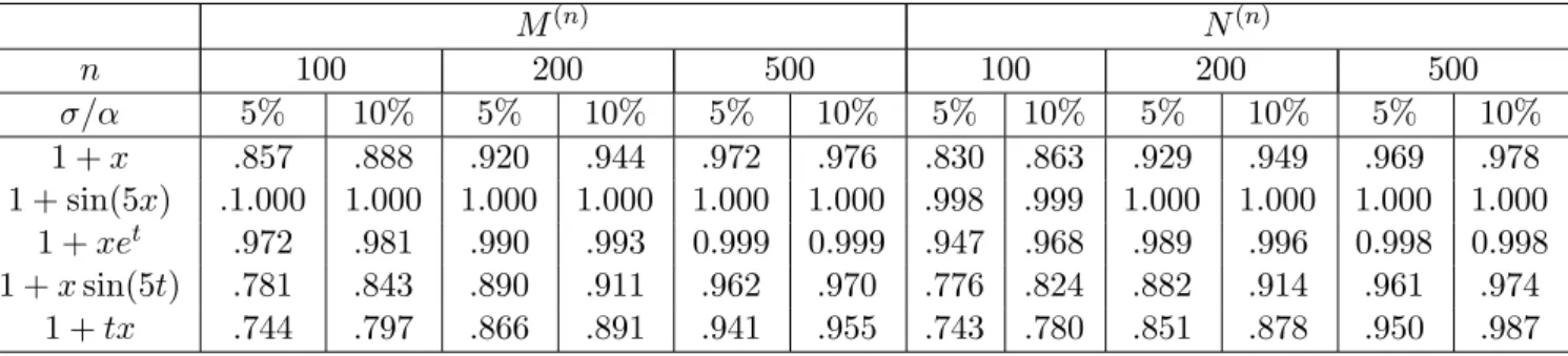
In Table 4.2 we present the corresponding rejection probabilities for the sample sizes n = 100,200 and 500. The results are directly comparable with the results in Table 3 of Dette and von Lieres und Wilkau (2003) for the corresponding test based on the statistic (3.15). From Thoereom 3.6 we expect some improvement in local power with respect to Pitman alternatives by the new procedure and these theoretical advantages are impressively reflected in our simulation study. We observe a substantial increase in power for the new tests. In most cases the improvement is at least approximately 15% and there are many cases, for which the power of the new test with 200 observations already exceeds the power of the test of Dette, von Lieres und Wilkau (2003) for 500 observations.
M(n) N(n)
n 100 200 500 100 200 500
σ/α 5% 10% 5% 10% 5% 10% 5% 10% 5% 10% 5% 10%
1 +x .857 .888 .920 .944 .972 .976 .830 .863 .929 .949 .969 .978 1 + sin(5x) .1.000 1.000 1.000 1.000 1.000 1.000 .998 .999 1.000 1.000 1.000 1.000
1 +xet .972 .981 .990 .993 0.999 0.999 .947 .968 .989 .996 0.998 0.998 1 +xsin(5t) .781 .843 .890 .911 .962 .970 .776 .824 .882 .914 .961 .974
1 +tx .744 .797 .866 .891 .941 .955 .743 .780 .851 .878 .950 .987
Table 4.2. Rejection probabilities of the tests, which reject the null hypothesis of homoscedasticity for large values of thes tatistics M(n) and N(n). The critical values are obtained by the asymptotic law (4.1) and (4.2), respectively.
4.2 Testing for the parametric form of the volatility
As pointed out previously, for a general null hypothesis the asymptotic distribution of the processes depends on the underlying diffusion (Xt)t∈[0,1] and cannot be used for the calculation of critical values (except in the problem of testing for homoscedasticity). However, conditional on (Xt)t∈[0,1]
the limiting processes in Theorem 3.3 and 3.5 are Gaussian and this suggests that the parametric bootstrap can be used to obtain critical values. In this paragraph we will investigate the finite sample performance of this approach. We explain this procedure for the process ( ˆMt)t∈[0,1], the corresponding bootstrap test for the process ( ˆNt)t∈[0,1] is obtained similarly. In a first step the least squares estimator ˆθmin = (ˆθ1min, . . . ,θˆdmin)T defined in (2.24) is determined. Then the process
√nMˆt is standardized by an estimate of the conditional variance s2t =µ−12(µ2−µ21)(1,−BtTD−1)
Z 1 0
Σt(s, Xs)ds (1,−BtTD−1)T
For the corresponding estimate, say ˆs2t, the random variables Bt und D are replaced by their empirical counterparts defined in Section 3, and the random elements in the matrix Σt(s, Xs) defined in (3.1) are replaced by the statistics
[nt]
X
k=1
(Xk
n −Xk−1
n )2 −→P Z t
0
σ2(s, Xs)ds
[nt]
X
k=1
σi2(k−1 n , Xk−1
n )(Xk
n −Xk−1
n )2 −→P Z t
0
σi2(s, Xs)σ2(s, Xs)ds
n
X
k=1
σj2(k−1 n , Xk−1
n )σ2i(k−1 n , Xk−1
n )(Xk
n −Xk−1
n )2 −→P Z 1
0
σj2(s, Xs)σi2(s, Xs)σ2(s, Xs)ds This yields the (standardized) Kolmogorov-Smirnov statistic
Zn = sup
t∈[0,1]
√nMˆt
ˆ st
(4.3)
In a second step data Xi/n∗(j) (i = 1, . . . , n; j = 1, . . . B) from the stochastic differential equation (1.1) with b(t, x) ≡ 0 and σ(t, x) = Pd
j=1θˆjminσj(t, x) are generated [note that this choice corre- sponds to the null hypothesis (2.5)]. These data are used to calculate the bootstrap analogues
Zn∗(1), . . . , Zn∗(B)
of the statistic Zn defined in (4.3). Finally the value of the statistic Zn is compared with the corresponding quantiles of the bootstrap distribution.
We have investigated the performance of this resampling procedure for the problem of testing various linear hypotheses, where the volatility function depends on the variable x. The sample sizes are againn = 100,200,500 andB = 500 bootstrap replications are used for the calculation of the critical values. In particular we compare the two procedures based on ( ˆMt)t∈[0,1] and ( ˆNt)t∈[0,1]
for testing the hypothesis
H¯0 : σ2(t, x) = ¯θx2 (4.4)
H0 : σ(t, x) =θx
In Table 4.3 we display the simulated level of the parametric bootstrap tests for various drift functions. We observe a better approximation of the nominal level by the test based on the process (Nt)t∈[0,1], in particular for small sample sizes. The Kolmogorov-Smirnov test based on the process ( ˆMt)t∈[0,1] yields a reliable approximation of the nominal level for sample sizes larger than 200, while the statistic based on the process ˆNt can already be recommended for n = 100.
The results for sample size n = 200, 500 demonstrate that for high frequency data as considered in this paper both tests yield a reliable approximation of the nominal level. In Table 4.4 we show the simulated rejection probabilities for the case b(t, x) = 2−x and the alternatives
σ2(t, x) = 1 +x2,1,5|x|3/2,5|x|,(1 +x)2
Mˆt Nˆt
n 100 200 500 100 200 500
b/α 5% 10% 5% 10% 5% 10% 5% 10% 5% 10% 5% 10%
0 .125 .195 .081 .135 .074 .133 .052 .110 .050 .099 .061 .114 2 .076 .126 .066 .107 .048 .096 .084 .132 .079 .124 .069 .117 x .094 .148 .071 .128 .048 .100 .069 .129 .057 .117 .054 .100 2−x .082 .133 .065 .112 .063 .117 .048 .088 .043 .101 .043 .097 xt .103 .166 .068 .130 .062 .116 .049 .103 .046 .099 .063 .105
Table 4.3. Simulated level of the bootstrap test for the hypothesis (4.4) based on the standardized Kolmogorov-Smirnov functional of the processes ( ˆMt)t∈[0,1] and ( ˆNt)t∈[0,1].
Mˆt Nˆt
n 100 200 500 100 200 500
σ2/α 5% 10% 5% 10% 5% 10% 5% 10% 5% 10% 5% 10%
1 +x2 .516 .587 .652 .720 .831 .885 .352 .467 .502 .627 .752 .828 1 .809 .862 .933 .955 .996 .998 .739 .838 .917 .960 .995 .997 5|x|3/2 .371 .516 .511 .638 .743 .838 .252 .310 .388 .534 .485 .598 5|x| .917 .882 .954 .970 .994 .997 .439 .551 .731 .858 .898 .949 (1 +x)2 .749 .815 .874 .920 .960 .976 .387 .500 .537 .751 .883 .934
Table 4.4. Simulated rejection probabilities of the bootstrap test for the hypothesis (4.4) based on the standardized Kolmogorov-Smirnov functional of the processes ( ˆMt)t∈[0,1] and ( ˆNt)t∈[0,1].
Note that the Kolmogorov-Smirnov test based on the process ( ˆMt)t∈[0,1] is substantially more powerful than the test based on the process ( ˆNt)t∈[0,1] which uses the squared differences. This superiority is partially bought by a worse approximation of the nominal level for smaller sample sizes [see the results for n = 100 and n = 200 in Table 4.3]. However, in the case b(t, x) = 2−x and n = 200, 500 both tests keep approximately their level, but the test based on ( ˆMt)t∈[0,1] is still substantially more powerful. Thus for high frequency data we recommend the application of the Kolmogorov-Smirinov test based on the process ( ˆMt)t∈[0,1].
It is also of interest to compare the power of the new tests with a bootstrap test, which was recently proposed by Dette, Podolskij and Vetter (2005) and is based on an estimate of the L2-distance
M2 = min
θ1,...,θd
Z 1 0
nσ2(t, Xt)−
d
X
j=1
θjσj2(t, Xt)o2
dt.
Because this test yield a rather accurate approximation of the nominal level [see Table 1 in this reference] we mainly consider the Kolmogorov-Smirnov test based on the process ( ˆNt)t∈[0,1] in our comparison. The results in the right part of Table 4.4 are directly comparable with the results displayed in Tabel 4 of Dette, Podolskij and Vetter (2005). We observe that in most cases the new Kolmogorov-Smirnov test yields a substantial improvement with respect to power. For the sample size n = 100 the procedure is more powerful for detecting the alternatives σ2(t, x) = 1; 1 +x2 and less powerful for the alternative σ2(t, x) = 5|x|3/2. For the remaining two alternatives the new test yields slightly better results. One the other hand the asymptotic advantages of the Kolmogorov-Smirnov test become more visible for larger sample sizes (n = 200, n = 500), where it outperforms the test based on the L2-distance in all cases. For example, the power of the test of Dette, Podolskij and Vetter (2005) with n = 500 observations is already achieved by the Kolmogorov-Smirnov test with n= 200 observations. Except for the alternative σ2(t, x) = 5|x|3/2 the power of the new test is substantially larger.
We finally note again that the power of the Kolmogorov-Smirnov test based on the process ( ˆMt)t∈[0,1] is even larger than the power obtained for ( ˆNt)t∈[0,1]. Thus for high frequeny data the new tests are a substantial improvement of the currently available procedure for testing the parametric form of the diffusion coefficient in a stochastic differential equation.
4.3 Data Example
In this paragraph we apply the test based on the process (Nt)t∈[0,1] to tick-by-tick data. As a specific example we consider the log returns of the excange rate between the EUR and the US dollar in 2004. The data were available for 10 weeks between February and April 2004 and approximately 710 log returns were recorded per week. A typical picture for the 4th and 8th week is depicted in Figure 4.1.
We applied the proposed procedures to test the hypotheses ¯H0:σ2(t, x) = ¯θ1, ¯H0 :σ2(t, x) = ¯θ1|x|, H¯0 : σ2(t, x) = ¯θ1x2 and ¯H0 : σ2(t, x) = ¯θ1 + ¯θ2x2. The corresponding p-values are depicted in Table 4.5. The null hypothesis ¯H0 :σ2(t, x) = ¯θ1 is cleary rejected in all cases. For the hypotheses H¯0 :σ2(t, x) = ¯θ1|x| and ¯H0 : σ2(t, x) = ¯θ1x2 the results do not indiate a clear structure. In the remaining case ¯H0 : σ2(t, x) = ¯θ1 + ¯θ2x2 we observe relatively large p-values, which gives some evidence for the null hypothesis in all weeks under consideration. Further details of this evaluation are available from the authors.
-0.002 -0.001 0.001 0.002
-0.002 -0.001 0.001 0.002
Figure 4.1. Log returns of the EUR/USD exchange rate for two different weeks.
week 1th 2th 3th 4th 5th 6th 7th 8th 9th 10th
n 714 714 713 714 714 714 708 714 718 710
σ2(t, x) =θ1 0.000 0.026 0.000 0.002 0.002 0.000 0.004 0.000 0.001 0.010 σ2(t, x) =θ1|x| 0.142 0.294 0.000 0.060 0.352 0.062 0.546 0.000 0.056 0.000 σ2(t, x) =θ1x2 0.748 0.714 0.000 0.976 0.774 0.368 0.634 0.000 0.710 0.000 σ2(t, x) =θ1 +θ2x2 0.880 0.996 0.886 0.994 0.978 0.986 0.968 0.974 0.966 0.988 Table 4.5. p-values of the test based on the process (Nt)t∈[0,1] for various hypotheses on the volatility function. The table shows the results for ten weeks. The second row shows the number of the available data at each week.

![Table 4.3. Simulated level of the bootstrap test for the hypothesis (4.4) based on the standardized Kolmogorov-Smirnov functional of the processes ( ˆ M t ) t ∈ [0,1] and ( ˆN t ) t ∈ [0,1] .](https://thumb-eu.123doks.com/thumbv2/1library_info/3637661.1502539/16.892.120.779.713.896/simulated-bootstrap-hypothesis-standardized-kolmogorov-smirnov-functional-processes.webp)
![Table 4.4. Simulated rejection probabilities of the bootstrap test for the hypothesis (4.4) based on the standardized Kolmogorov-Smirnov functional of the processes ( ˆ M t ) t ∈ [0,1] and ( ˆN t ) t ∈ [0,1] .](https://thumb-eu.123doks.com/thumbv2/1library_info/3637661.1502539/17.892.114.789.101.277/simulated-rejection-probabilities-bootstrap-hypothesis-standardized-kolmogorov-functional.webp)

