A Strongly Polynomial Algorithm for Linear Exchange Markets

arXiv:1809.06266v2 [cs.DS] 3 Nov 2018

A Strongly Polynomial Algorithm for Linear Exchange Markets

Jugal Garg

^∗

jugal@illinois.edu

László A. Végh

^†

l.vegh@lse.ac.uk November 6, 2018

Abstract

We present a strongly polynomial algorithm for computing an equilibrium in Arrow-Debreu exchange markets with linear utilities. The main measure of progress is identifying a set of edges that must correspond to best bang-per-buck ratios in every equilibrium, called the revealed edge set. We use a variant of the combinatorial algorithm by Duan and Mehlhorn [12] to identify a new revealed edge in a strongly polynomial number of iterations. Every time a new edge is found, we use a subroutine to identify an approximately best possible solution corresponding to the current revealed edge set. Finding the best solution can be reduced to solving a linear program.

Even though we are unable to solve this LP in strongly polynomial time, we show that it can be approximated by a simpler LP with two variables per inequality that is solvable in strongly polynomial time.

1 Introduction

The exchange market model has been introduced by Walras in 1874 [41]. In this model, a set of agents arrive at a market with an initial endowment of divisible goods and have a utility function over allocations of goods. Agents can use their revenue from selling their initial endowment to purchase their preferred bundle of goods. In a market equilibrium, the prices are such that each agent can spend their entire revenue on a bundle of goods that maximizes her utility at the given prices, and all goods are fully sold.

The celebrated result of Arrow and Debreu [2] shows the existence of an equilibrium for a broad class of utility functions. Computational aspects have been already addressed since the 19th century, see e.g. [3], and polynomial time algorithms have been investigated in the theoretical computer science community over the last twenty years; see the survey [4] for early work, and the references in [17] for more recent developments.

In this paper we study the case where all utility functions are linear. Linear market models have been extensively studied since 1950s; see [8] for an overview of earlier work. These models are also appealing from a combinatorial optimization perspective due to their connection to classical network flow models and their rich combinatorial structure. A well-studied special case of the exchange market is the Fisher market setting, where every buyer arrives with a fixed budget instead of an endowment of goods. Using network flow techniques, Devanur et al. [9] gave a polynomial-time combinatorial algorithm that was followed by a series of further such algorithms [20,

36], including strongly polynomial

ones [30,

39]. In contrast, for the general exchange market the first combinatorial algorithm was

developed much later by Duan and Mehlhorn [12], and no strongly polynomial algorithm has been known thus far.

Strongly polynomial algorithms and rational convex programs Assume that a problem is given by an input of N rational numbers given in binary description. An algorithm for such a problem is strongly polynomial (see [22, Section 1.3]), if it only uses elementary arithmetic operations (addition, comparison, multiplication, and division), and the total number of such operations is bounded by

∗University of Illinois at Urbana-Champaign. Supported by an NSF CRII Award 1755619.

†London School of Economics and Political Science. Supported by the ERC Starting Grant ScaleOpt.

poly(N ). Further, the algorithm is required to run in polynomial space : that is, the size of the numbers occurring throughout the algorithm remain polynomial in the size of the input. Here, the size of a rational number p/q with integers p and q is defined as ⌈log

₂

(|p| + 1)⌉ + ⌈log

₂

(|q| + 1)⌉.

It is a major open question to find a strongly polynomial algorithm for linear programming. Such algorithms are known for special classes of linear optimization problems. We do not present a com- prehensive overview here but only highlight some examples: systems of linear equations with at most two nonzero entries per inequality [1,

5, 26]; minimum cost circulations e.g. [21, 29, 33]; LPs with

bounded entries in the constraint matrix [34,

35]; generalized flow maximization [28,40], and variants

of Markov Decision Processes [42,

44].

For nonlinear convex optimization, only sporadic results are known. The relevance of certain market equilibrium problems in this context is that they can be described by rational convex programs, where a rational optimal solution exists with encoding size bounded in the input size (see [37]). This property gives hope for finding strongly polynomial algorithms.

The linear Fisher market equilibrium can be captured by two different convex programs, one by Eisenberg and Gale [15], and one by Shmyrev [32]. These are special cases of natural convex extensions of classical network flow models [38,

39]. In particular, the second model is a network flow problem

with a separable convex cost function; [39] provides a strongly polynomial algorithm for the linear Fisher market using this general perspective.

The exchange market model cannot be described by such simple convex programs. A rational convex program was given in [8], but the objective is not separable and hence the result in [39] cannot be applied. Previous convex programs [6,

23, 27] included nonlinear constraints and did not appear

amenable for a combinatorial approach (see [8] for an overview).

Model Let A be the set of n agents. Without loss of generality, we can assume that there is one unit in total of each divisible good, and that there is a one-to-one correspondence between agents and goods: agent i brings the entire unit of the i-th good, g

_i

to the market. If agent i buys x

_ij

units of good g

_j

, her utility is

P

j

u

_ij

x

_ij

, where u

_ij

is the utility of agent i for a unit amount of good g

_j

. Given prices p = (p

_i

)

_i∈A

, the bundle that maximizes the utility of agent i is any choice of maximum bang-per-buck goods, that is, goods that maximize the ratio u

_ij

/p

_j

. The prices p and allocations (x

_ij

)

_i,j∈A

form a market equilibrium, if (i)

P

i∈A

x

_ij

= 1 for all j, that is, every good is fully sold; (ii) p

_i

=

P

j∈A

p

_j

x

_ij

for all i, that is, every agent spends her entire revenue; and (iii) x

ij

> 0 implies that u

ij

/p

j

= max

_k

u

_ik

/p

_k

, that is, all purchases maximize bang-per-buck.

Algorithms for the linear exchange market A finite time algorithm based on Lemke’s scheme [25]

was obtained by Eaves [13]. A necessary and sufficient condition for the existence of equilibrium was described by Gale [16]. The first polynomial-time algorithms for the problem were given by Jain [23]

using the ellipsoid method and by Ye [43] using an interior point method. The combinatorial algorithm of Duan and Mehlhorn [12] builds on the algorithm [9] for linear Fisher markets. An improved variant was given in [11] with the current best weakly polynomial running time O(n

⁷

log

³

(nU )), assuming all u

_ij

values are integers between 0 and U . A main measure of progress in these algorithms is the increase in prices. However, the upper bound on the prices depends on the u

_ij

values; therefore, such an analysis can only provide a weakly polynomial bound. The existence of a strongly polynomial algorithm is described in [12] as a major open question. There is a number of simple algorithms for computing an approximate equilibrium [10,

18,19,24], but these do not give rise to polynomial-time

exact algorithms.

Our result We provide a strongly polynomial algorithm for linear exchange markets with running

time O(n

⁹

m log

²

n), where m is the number of pairs (i, g

_j

) with u

_ij

> 0; clearly, m ≤ n

²

. Let us give

an overview of the main ideas and techniques. Let F

^∗

denote the set of edges (pairs of agents and

goods) that correspond to a best bang-per-buck transaction in every equilibrium. In the algorithm, we

maintain a set F ⊆ F

^∗

called revealed edges, and the main progress is adding a new edge in strongly

polynomial time. At a high level, this approach resembles that of [39], which extends Orlin’s approach

for minimum-cost circulations [29].

In a money allocation (p, f ), (p

_i

)

_i∈A

is a set of prices and (f

_ij

)

_i,j∈A

represent the amount of money paid for good g

_j

by agent i; f

_ij

may only be positive for maximum bang-per-buck pairs. In the algorithm we work with a money allocation where goods may not be fully sold and agents may have leftover money; we let ks(p, f )k

₁

denote the total surplus money left, and ks(p, f )k

∞

the maximum surplus of any good. It can be shown that if f

ij

> ks(p, f )k

₁

in a money allocation, then (i, g

j

) ∈ F

^∗

. This is analogous to the method of identifying abundant arcs for minimum cost flows by Orlin [29].

We use a variant of the Duan-Mehlhorn (DM) algorithm to identify abundant arcs. We show that the potential φ(p, f ) = ks(p, f )k

_∞

/(

Q

j

p

j

)

^1/n

decreases geometrically in the algorithm; from this fact, it is not difficult to see that an arc with f

_ij

> ks(p, f )k

₁

appears in a strongly polynomial number of iterations, yielding the first revealed arc. We need to modify the DM algorithm [12] so that, among other reasons, the potential decreases geometrically when we run the algorithm starting with any arbitrary price vector p; see Remark

5.1

in Section

5

for all the differences.

To identify subsequent revealed arcs, we need a more flexible framework and a second subroutine.

We work with the more general concept of F -allocations, where the money amount f

ij

could be negative if (i, g

_j

) ∈ F. This is a viable relaxation since an F -equilibrium (namely, a market equilibrium with possibly negative allocations in F ) can be efficiently turned into a proper market equilibrium, provided that F ⊆ F

^∗

. Given a set F of revealed arcs, our Price Boost subroutine finds an approximately optimal F -allocation using only edges in F . Namely, the subroutine finds an F-equilibrium if there exists one; otherwise, it finds an F -allocation that is zero outside F, and subject to this, it approximately minimizes φ(p, f ). This will provide the initial prices for the next iteration of the DM subroutine.

Since DM decreases φ(p, f ) geometrically, after a strongly polynomial number iterations it will need to send a substantial amount of flow on an edge outside F, providing the next revealed edge.

Let us now discuss the Price Boost subroutine. The analogous subproblem for Fisher markets in [39] reduces to a simple variant of the Floyd-Warshall algorithm. For exchange markets, we show that optimizing φ(p, f ) can be captured by a linear program. A strongly polynomial LP algorithm would therefore immediately provide the desired subroutine. Alas, this LP is not contained in any special class of LP where strongly polynomial algorithms are currently known.

We will exploit the following special structure of the LP. We can eliminate the f

_ij

variables and only work with price variables. The objective is to maximize the sum of all variables over a feasible set of the form P ∩ P

^′

. The first polyhedron P is defined by inequalities with one positive and one nonnegative variable per inequality. The constraint matrix defining the second polyhedron P

^′

is what we call a Z

₊

-matrix: all off-diagonal elements are nonpositive but all column sums are nonnegative.

This corresponds to a submatrix of the transposed of a weighted Laplacian matrix. In case we only had constraints of the form P , classical results [1,

5,26] would provide a strongly polynomial running

time. To deal with the constraints defining P

^′

, we approximate our LP by a second LP that can be solved in strongly polynomial time.

More precisely, we replace the second polyhedron P

^′

by Q such that P

^′

⊆ Q ⊆ n

²

P

^′

, and that Q is also a system with one positive and one nonnegative variable per inequality. Thus, the algorithms [1,

5,26] are applicable to maximize the sum of the variables over

P ∩ Q in strongly polynomial time.

For an optimal solution p, the vector ¯ p/n ¯

²

is feasible to the original LP and the objective value is within a factor n

²

of the optimum. For the purposes of identifying a new revealed arc in the algorithm, such an approximation of the optimal φ(p, f ) value already suffices.

The construction of the approximating polyhedron Q is obtained via a general method applicable for systems given by Z

₊

-matrices. We show that for such systems, Gaussian elimination can be used to generate valid constraints with at most two nonzero variables per row. Moreover, we show that the intersection of all relevant such constraints provides a good approximation of the original polyhedron.

The rest of the paper is structured as follows. Section

2

introduces basic definitions and notation.

Section

3

describes the overall algorithm by introducing the notion of F -allocations, the main potential, and the two necessary subroutines. Section

4

proves the lemmas necessary for identifying revealed edges. Section

5

presents the first of these two subroutines, a variant of the Duan-Mehlhorn algorithm.

Section

6

shows how the second subroutine, Price Boost, can be reduced to solving an LP. Section

7

exhibits the polyhedral approximation result for Z

₊

-matrices. Section

8

concludes with some open

questions.

2 Preliminaries

For a positive integer t, we let [t] := {1, 2, . . . , t}, and for k < t, we let [k, t] := {k, k + 1, . . . , t}. For a vector a ∈

Rⁿ

, we let

kak

₁

:=

n

X

i=1

|a

i

|, kak

₂

:=

v u u t

n

X

i=1

a

²_i

, and kak

∞

:= max

i∈[n]

|a

i

|

denote the ℓ

₁

, ℓ

₂

, and ℓ

∞

-norms, respectively. Further, we let supp(a) ⊆ [n] denote the support of the vector a ∈

Rⁿ

, that is, supp(a) := {i ∈ [n] | a

_i

6= 0}. For a subset S ⊆ [n], we let a(S) :=

P

i∈S

a

_i

. The linear exchange market We let A := [n] denote the set of agents, G := {g

₁

, g

₂

, . . . , g

_n

} denote the set of goods, and u

_ij

≥ 0 denote the utility of agent i for a unit amount of good g

_j

. Let E ⊆ A × G denote the set of pairs (i, g

_j

) such that u

_ij

> 0; let m := |E|. We will assume that for each i ∈ A there exists a g

j

∈ G such that u

ij

> 0, and for each g

j

∈ G there exists an i ∈ A such that u

ij

> 0. Hence, m ≥ n.

The goods are divisible and there is one unit of each in total. Agent i arrives to the market with her initial endowment comprising exactly the unit of good g

i

. As mentioned in the introduction, the general case with an arbitrary set of goods and arbitrary initial endowments can be easily reduced to this setting; see [8,

23].

Let p = (p

j

)

gj∈G

denote the prices where p

j

is the price of good g

j

. Given prices p, we let α

_i

:= max

gk∈G

u

_ik

p

_k

, ∀i ∈ A.

For each agent i ∈ A, the goods satisfying equality here are called maximum bang-per-buck (MBB) goods; for such a good g

_j

, (i, g

_j

) is called an MBB edge. We let MBB(p) ⊆ E denote the set of MBB edges at prices p.

Definition 2.1. Let f = (f

_ij

)

_i∈A,gj∈G

denote the money flow where f

_ij

is the money spent by agent i on good g

j

. We say that (p, f ) is a money allocation if

(i) p > 0, and f ≥ 0;

(ii) supp(f ) ⊆ MBB(p);

(iii)

P

gj∈G

f

_ij

≤ p

_i

for every agent i ∈ A;

(iv)

P

i∈A

f

_ij

≤ p

_j

for every good g

_j

∈ G.

For the money allocation (p, f ), the surplus of agent i is defined as c

_i

(p, f ) := p

_i

−

X

gj∈G

f

_ij

,

and the surplus of good g

_j

∈ G is defined as

s

j

(p, f ) := p

j

−

X

i∈A

f

ij

.

Parts (iii) and (iv) in the definition of the money allocation require that the surplus of all agents and goods are nonnegative. We let c(p, f ) := (c

_i

(p, f ))

_i∈A

and s(p, f ) := (s

_j

(p, f ))

_gj∈G

denote the surplus vectors of the agents and the goods, respectively. Clearly, ks(p, f )k

₁

= kc(p, f )k

₁

, and ks(p, f )k

_∞

≤ ks(p, f )k

₁

≤ nks(p, f )k

∞

.

Definition 2.2. A money allocation (p, f ) is called a market equilibrium if ks(p, f )k

₁

= 0.

Existence of an equilibrium A market equilibrium may not exist for certain inputs. For example, consider a market with 3 agents and 3 goods, where agent i brings one unit of good g

_i

for i = 1, 2, 3.

Let E = {(1, g

1

), (1, g

₂

), (2, g

₃

), (3, g

₃

)}. Clearly, in this market, at any prices, Agent 3 will consume the entire g

₃

. If p

₂

> 0, then Agent 2 will demand a non-zero amount of g

₃

, and therefore no market equilibrium exists.

A necessary and sufficient condition for the existence of an equilibrium can be given as follows. Let us define the directed graph (A, E), where ¯ (i, j) ∈ E ¯ if and only if u

_ij

> 0 (that is, if (i, g

_j

) ∈ E).

Lemma 2.1 ([16,

8]).

There exists a market equilibrium if and only if for every strongly connected component S ⊆ A of the digraph (A, E), if ¯ |S| = 1, then there is a loop incident to the node in S.

This condition can be easily checked in strongly polynomial time. Further, it is easy to see that if the above condition holds, then finding an equilibrium in an arbitrary input can be reduced to finding an equilibrium in an input where the digraph (A, E) ¯ is strongly connected. Thus, we will assume the following throughout the paper:

The graph (A, E) ¯ is strongly connected. (⋆)

3 The overall algorithm

In this section, we describe the overall algorithm. We formulate the statements that are needed to prove our main theorem:

Theorem 3.1. There exists a strongly polynomial algorithm that computes a market equilibrium in linear exchange markets in time O(n

⁹

m log

²

n).

We start by introducing the concepts of revealed edges, F-allocations, and balanced F -flows.

3.1 Revealed edges

Throughout the paper, we let F

^∗

⊆ E denote the set of edges (i, g

_j

) ∈ E that are MBB edges for every market equilibrium (p, f ). In the algorithm, we will maintain a subset of edges F ⊆ F

^∗

that will be called the revealed edge set. This is initialized as F = ∅.

Definition 3.2. For an edge set F ⊆ E, (p, f ) is an F -money allocation, or F -allocation in short, if (i) p > 0, and f

_ij

≥ 0 for (i, g

_j

) ∈ / F ;

(ii) supp(f ) ∪ F ⊆ MBB(p);

(iii)

P

gj∈G

f

ij

≤ p

i

for every agent i ∈ A;

(iv)

P

i∈A

f

_ij

≤ p

_j

, for every good g

_j

∈ G.

An F-allocation is called an F -equilibrium if ks(p, f )k

₁

= 0.

Note that f

ij

could be negative for (i, g

j

) ∈ F . A ∅-allocation simply corresponds to a money allocation.

The main progress step in the algorithm will be adding new edges to F . This will be enabled by the following lemma; the proof is deferred to Section

4.

Lemma 3.1. Let F ⊆ F

^∗

, and let (p, f ) be an F -allocation. If f

_kℓ

> ks(p, f )k

₁

for an edge (k, g

_ℓ

) ∈ E, then (k, g

_ℓ

) ∈ F

^∗

.

Our algorithm will obtain an F-equilibrium. Whereas an F -equilibrium is not necessarily an equilibrium, the following holds true:

Lemma 3.2. Let F ⊆ F

^∗

, and assume we are given an F -equilibrium (p, f ). Then a market equilibrium (p, f

^′

) can be obtained in O(nm) time.

We let

Final-Flow

(p) denote the algorithm as in the Lemma. This is a maximum flow computa-

tion in an auxiliary network, as described in the proof in Section

4.

Algorithm 1: Arrow-Debreu Equilibrium

Input : Set A of agents, set G of goods, and utilities (u

_ij

)

_i∈A,gj∈G

Output: Market equilibrium (p, f )

1

F ← ∅;

2

repeat

3

(ˆ p, f ˆ ) ←

Boost

(F)

// Theorem 3.4

4

(p, f ) ←

DM

(F, p) ˆ

// Theorem 3.5

5

F ← F ∪ {(i, g

j

) | f

_ij

> ks(p, f )k

1

}

// Lemma 3.1 6

until ks(p, f )k

₁

= 0

7

f ←

Final-Flow

(p)

// Lemma 3.2

8

return (p, f )

3.2 Balanced flows

Balanced flows play a key role in the Duan-Mehlhorn algorithm [12], as well as in previous algorithms for Fisher market models [9,

20,36]. We now introduce the natural extension for

F -allocations.

Definition 3.3. Given an edge set F ⊆ E and prices p, we say that (p, f ) is a balanced F -flow, if (p, f ) is an F-allocation that minimizes ks(p, f )k

₁

, and subject to that, it minimizes kc(p, f )k

₂

. Lemma 3.3. Given F ⊆ E and prices p such that F ⊆ MBB(p), a balanced F-flow can be computed in O(n

²

m) time.

We let

Balanced

(F, p) denote the subroutine guaranteed by the Lemma. The proof in Ap- pendix

A.1

follows the same lines as in [9,

12], by computing at most

n maximum flows in an auxiliary graph.

3.3 The algorithm

The overall algorithm is presented in Algorithm

1. The main progress is gradually expanding a revealed

edge set F ⊆ F

^∗

, initialized as F = ∅. Every cycle of the algorithm performs the subroutines

Boost

(F ) and

DM

(F, p), and at least one new edge is added to ˆ F at every such cycle. Once an F-equilibrium is obtained for the current F , we use the subroutine

Final-Flow

(p) as in Lemma

3.2

to compute a market equilibrium.

We now introduce the key potential measures used in analysis. For an F -allocation (p, f ), we define φ(p, f ) := ks(p, f )k

∞

(

Qn

j=1

p

_j

)

^1/n

.

Note that this is invariant under scaling, i.e. φ(p, f ) = φ(αp, αf ) for any α > 0. Further, (p, f ) is an F -equilibrium if and only if φ(p, f ) = 0. For a given F ⊆ F

^∗

, we define

Ψ(F ) := min{φ(p, f ) : (p, f ) is an F -allocation, supp(f) ⊆ F }. (1) Theorem 3.4. There exists a strongly polynomial time algorithm that for any input F ⊆ E, returns in time O(n

⁴

log

²

n) an F -allocation (ˆ p, f ˆ ) with supp( ˆ f ) ⊆ F such that Ψ(F ) ≤ φ(ˆ p, f) ˆ ≤ (n − 1)

²

Ψ(F).

The algorithm in the theorem will be denoted as

Boost

(F), and is described in Section

6. In

particular, if Ψ(F) = 0, then

Boost

(F) returns an F -equilibrium.

The second main subroutine

DM

(F, p), is a variant of the Duan-Mehlhorn algorithm [12], de- ˆ

scribed in Section

5. As the input, it uses the prices

p ˆ obtained in the F -allocation (ˆ p, f) ˆ returned

by

Boost

(F ), and outputs an F -allocation (p, f ) such that either ks(p, f )k

₁

= 0, that is, an F-

equilibrium, or it is guaranteed that f

_ij

> ks(p, f )k

₁

for some (i, g

_j

) ∈ E \ F connecting two different

connected components of F . Such an edge (i, g

_j

) can be added to F by Lemma

3.1. The following

simple lemma asserts the existence of such an edge.

Lemma 3.4. Let (p, f ) be an F -allocation such that φ(p, f ) < Ψ(F )/(n(m+1)). Then, f

_ij

> ks(p, f )k

₁

for at least one edge (i, g

_j

) ∈ E \ F such that i and g

_j

are in two different undirected connected components of F.

Proof. For a contradiction, assume f

_ij

≤ ks(p, f )k

₁

for every (i, g

_j

) ∈ E \ F where i and g

_j

are in different connected components of F . Let us define f

^′

as follows. We start by setting f

^′

= f ; then, for every (i, g

_j

) ∈ E \ F where i and g

_j

are in the same component, we reroute f

_ij

units of flow from i to g

_j

using a path in F . Such a path may contain both forward and reverse edges; we increase the flow on forward edges and decrease it on reverse edges. Further, we set f

_ij^′

:= 0 for (i, g

_j

) ∈ E \ F if i and g

_j

are in different connected components of F . The assumption yields

ks(p, f

^′

)k

∞

≤ ks(p, f

^′

)k

₁

≤ (m + 1)ks(p, f )k

₁

≤ n(m + 1)ks(p, f )k

∞

, and therefore

φ(p, f

^′

) ≤ n(m + 1)φ(p, f ) < Ψ(F ), a contradiction to the definition of Ψ(F ), since supp(f

^′

) ⊆ F.

Theorem 3.5. There exists a strongly polynomial O(n

⁸

m log

²

n) time algorithm, that, for a given F ⊆ E and prices p, computes an ˆ F -allocation (p, f ) such that

φ(p, f ) ≤ φ(ˆ p, f) ˜ n

⁴

(m + 1) , where f ˜ is the balanced flow computed by

Balanced

(F, p). ˆ

The algorithm

DM

(F, p) given in Section ˆ

5

will satisfy the assertion of this theorem. Using these claims, we are ready to prove Theorem

3.1.

Proof of Theorem

3.1.

By Lemma

3.4, the number of connected components of

F decreases after every cycle of Algorithm

1; thus, the total number of cycles is

≤ 2n − 1. Consider any cycle. Let (ˆ p, f ˆ ) denote that F -allocation returned by

Boost

(F ) with φ(ˆ p, f ˆ ) ≤ (n − 1)

²

Ψ(F), and let (ˆ p, f ˜ ) denote the balanced F -flow at prices p. Then, ˆ

ks(ˆ p, f ˜ )k

∞

≤ ks(ˆ p, f ˜ )k

₁

≤ ks(ˆ p, f ˆ )k

₁

≤ nks(ˆ p, f ˆ )k

∞

,

since (ˆ p, f ˜ ) minimizes ks(ˆ p, f)k ˜

₁

among all F -allocations. Therefore φ(ˆ p, f ˜ ) < n

³

Ψ(F ). Theorem

3.5

guarantees that

DM

(F, p) finds an ˆ F -allocation (p, f ) with φ(p, f ) < Ψ(F )/(n(m + 1)). Lemma

3.4

guarantees that F is extended by at least one new edge in this cycle. The overall running time estimation is dominated by the running time estimation of the calls to

DM

.

4 F -allocations and F -equilibria

This section is devoted to the proof of the Lemmas

3.1

and

3.2, which enable us to add new edges to

the revealed set F , as well as to convert an F -equilibrium to an equilibrium.

Proof of Lemma

3.1.

The claim is obvious if (k, g

_ℓ

) ∈ F ; for the rest of the proof we therefore assume (k, g

_ℓ

) ∈ / F . Let (p

^′

, f

^′

) be a market equilibrium. Every edge in F is an MBB-edge for (p, f ) by the definition of an F -allocation, and also for (p

^′

, f

^′

) because of F ⊆ F

^∗

. Since equilibrium prices are scale invariant in linear exchange markets, we can assume that p

^′_ℓ

= p

_ℓ

. Let T ⊆ G be the set of goods whose prices at p

^′

are at least the prices at p, i.e., T := {g

j

∈ G | p

^′_j

≥ p

_j

}. Clearly, g

_ℓ

∈ T . Let Γ

_p^′

(T ) be the set of agents who have MBB edges to goods in T at p

^′

, i.e.,

Γ

_p^′

(T ) := {i ∈ A | ∃g

j

∈ T, (i, g

_j

) ∈ MBB(p

^′

)} .

Observe that agents of Γ

_p^′

(T ) do not have MBB edges to goods in G \ T when prices are p.

For a contradiction, suppose (k, g

_ℓ

) ∈ / MBB(p

^′

). In that case, it follows that k 6∈ Γ

_p^′

(T ). Indeed, if there existed a good g

_j

∈ T such that (k, g

_j

) ∈ MBB(p

^′

), then we would get u

_kℓ

/p

_ℓ

= u

_kℓ

/p

^′_ℓ

<

u

_ij

/p

^′_j

≤ u

_ij

/p

_j

, a contradiction to (k, g

_ℓ

) ∈ MBB(p).

Consider the goods in T at prices p. Since no good is oversold, we have

X

i∈A,gj∈T

f

_ij

≤ p(T) .

Also note that f

_ij

≥ 0 whenever i ∈ A \ Γ

_p^′

(T ) and g

_j

∈ T. This is because f

_ij

could be negative only on edges in F ; however, for every (i, g

_j

) ∈ F such that g

_j

∈ T , we must have i ∈ Γ

_p^′

(T ), since all edges in F have to be MBB in every equilibrium. Therefore, the previous inequality implies

X

i∈Γ_p′(T),gj∈T

f

_ij

+ f

_kl

≤ p(T ) .

The agents in Γ

_p^′

(T ) do not have MBB edges at price p to goods in G \ T , thus, the first term in the left hand side is the total money they spend. Since their total surplus is at most ks(p, f )k

₁

, we obtain

p(Γ

_p^′

(T )) ≤ p(T ) − f

_kℓ

+ ks(p, f )k

₁

.

Using f

_kℓ

> ks(p, f )k

₁

and breaking p(Γ

_p^′

(T )) into two parts, we can rewrite the above as

X

j∈Γ_p′(T),gj6∈T

p

_j

<

X

j /∈Γ_p′(T),gj∈T

p

_j

. (2)

Let us now examine the market equilibrium (p

^′

, f

^′

), where f

^′

≥ 0 and f

_ij^′

> 0 is allowed only for the MBB edges at p

^′

. Since every agent spends their budget exactly at equilibrium, we have

p

^′

(Γ

_p^′

(T )) =

X

i∈Γ_p′(T),gj∈G

f

_ij^′

.

Further, since there are no MBB edges at prices p

^′

from agents outside Γ

_p^′

(T ) to goods in T , we obtain p

^′

(Γ

_p^′

(T )) =

X

i∈Γ_p′(T),gj∈G

f

_ij^′

≥

X

i∈Γ_p′(T),gj∈T

f

_ij^′

= p

^′

(T ) .

Again we can rewrite the above as

X

j∈Γ_p′(T),gj6∈T

p

^′_j

≥

X

j /∈Γ_p′(T),gj∈T

p

^′_j

. (3)

Now, since p

^′_j

≥ p

_j

for g

_j

∈ T and p

^′_j

< p

_j

for g

_j

6∈ T , (2) and (3) give a contradiction.

We formulate a simple corollary that will be needed in the proof of Lemma

3.2.

Corollary 4.1. If F ⊆ F

^∗

, then for every F -equilibrium f , supp(f ) ⊆ F

^∗

.

Proof of Lemma

3.2.

An F-equilibrium (p, f ) may not be a market equilibrium since f can have neg- ative values on some edges in F . If that is the case, we find a flow f ˜ such that (p, f ˜ ) is a market equilibrium as follows.

Let us construct the network N (p) on vertex set A ∪ G ∪ {s, t}, where s is a source node and t is a sink node, and the following set of edges: (s, i) with capacity p

i

for each i ∈ A, (g

j

, t) with capacity p

_j

for each g

_j

∈ G, and (i, g

_j

) with infinite capacity for each (i, g

_j

) ∈ MBB(p). Let us use Orlin’s algorithm [31] to obtain a maximum s − t flow f ˜ in N (p) in time O(nm).

If f ˜ saturates all edges out of s (equivalently, all edges into t), then clearly (p, f ˜ ) is a market equilibrium. We will show that this is indeed the case.

Let (p

^′

, f

^′

) be an equilibrium. Since equilibrium prices are invariant to scaling by a positive constant, we can assume that

P

gj∈G

p

^′_j

=

P

gj∈G

p

_j

. If p

^′

= p, then clearly (p, f ˜ ) is an equilibrium. For the

other case, p

^′

6= p, let E ¯ := F ∪ supp(f ), and let E

^′

:= MBB(p

^′

). Corollary

4.1

and the definition of F

^∗

imply E ¯ ⊆ F

^∗

⊆ E

^′

.

Next, let α := max

_gj∈G

{p

^′_j

/p

_j

}, and S := {j ∈ G | p

^′_j

/p

_j

= α}. Let Γ(S) be the set of agents who have at least one MBB edge to goods in S when prices are p

^′

, i.e.,

Γ(S) = {i ∈ A | ∃g

_j

∈ S, (i, g

_j

) ∈ E

^′

}.

We must have

X

i∈Γ(S)

p

^′_i

≥

X

gj∈S

p

^′_j

. (4)

Now consider the connected components of the bipartite graph (A ∪ G, E). Since ¯ E ¯ ⊆ E

^′

, there are connected components C

₁

, . . . , C

_ℓ

of (A ∪ G, E) ¯ such that

S_ℓ

k=1

(G ∩ C

_k

) = S. Furthermore, we also have

S_ℓ

k=1

(A ∩ C

_k

) = Γ(S), because prices of goods in S are increased by the largest factor when we go from p to p

^′

, and E ¯ ⊆ E

^′

. At the F -equilibrium (p, f ), we have

X

i∈Γ(S)

p

_i

=

X

gj∈S

p

_j

. (5)

The equations (4) and (5) imply that

P

i∈Γ(S)

p

^′_i

=

P

gj∈S

p

^′_j

and S = {g

j

∈ G | j ∈ Γ(S)}, i.e., the set of goods brought by agents in Γ(S) is exactly equal to S. This further implies that f

^′

for agents in Γ(S) and for goods in S is supported only on the MBB(p) edges between them, and hence f ˜ must saturate all agents in Γ(S) (and equivalently, all goods in S) because the set of MBB edges between Γ(S) and S remains same at p and p

^′

. Next, we remove the agents in Γ(S) and goods in S, and repeat the same analysis on the remaining set of agents and goods. This proves that (p, f ˜ ) is a market equilibrium.

5 The Duan-Mehlhorn (DM) subroutine

In this section, we present a variant of the Duan-Mehlhorn (DM) algorithm [12] as a subroutine DM(F, p) ˆ in Algorithm

2. The input is a revealed edge set

F and prices p ˆ such that F ⊆ MBB(ˆ p), and the output is either an F -equilibrium, or an F -allocation (p, f ) where f

_ij

> ks(p, f )k

₁

for some (i, g

_j

) ∈ E \ F connecting two different components of F. The modifications compared to the original DM algorithm are listed in Remark

5.1. We now provide a description where the subroutine terminates once

an arc with f

_ij

> ks(p, f )k

₁

is identified. The variant as required in Theorem

3.5

can be obtained by simply by removing the termination condition, and letting the algorithm run for O(n

⁶

log

²

n) iterations of the outer loop.

We call one execution of the outer loop a phase, and one execution of the inner loop an iteration.

Algorithm

2

first computes a balanced flow f using the subroutine

Balanced

(F, p) as in Lemma

3.3.

Then, the agents are sorted in decreasing order of surplus. Without loss of generality, we assume that c

₁

(p, f ) ≥ · · · ≥ c

_n

(p, f ). Then, we find the smallest ℓ for which the ratio c

_ℓ

(p, f )/c

_ℓ+1

(p, f ) is more than 1 + 1/n. If there is no such ℓ then we let ℓ := n. Let S be the set of first ℓ agents, and let Γ(S) be the set of goods for which there is a non-zero flow from agents in S. Since f is balanced, the agents outside S have zero flow to goods in Γ(S), i.e., f

_ij

= 0, ∀i 6∈ S, g

_j

∈ Γ(S) and the surplus of every good in Γ(S) is zero. We set γ to 1 before we go into the inner loop.

Next, the algorithm runs the inner loop where it increases the prices of goods in Γ(S) and the flow between agents in S and goods in Γ(S) by a multiplicative factor x ≥ 1 until one of the three events occurs. Observe that except for the MBB edges (i, g

_j

) where i / ∈ S, g

_j

∈ Γ(S), all MBB edges remain MBB with this price change, and the surplus of every good in Γ(S) remains zero. When prices of goods in Γ(S) increase, an edge (i, g

_j

) from i ∈ S and g

_j

6∈ Γ(S) can become MBB. We need to stop when such an event occurs in order to maintain an F -allocation. This is captured by Event 1. In Event 2, we stop when the surplus of an agent i ∈ S becomes equal to either the surplus of an agent i

^′

6∈ S or zero.

Let us note that c

_i

(p, f ) ≥ 0 is maintained throughout; we use the expression max{max

_{i /∈S}

c

_i

(p, f ), 0}

to also cover the possible case S = [n]. In Event 3, we stop when γx becomes 1 + 1/(56e

²

n

³

).

If Event 1 occurs, then we have a new MBB edge (a, g

_b

) from a ∈ S to g

_b

6∈ Γ(S). Using this new

edge, it is now possible to decrease the surplus of agent a and increase the surpluses of agents i 6∈ S

Algorithm 2: DM(F, p) ˆ

Input : Utilities (u

_ij

)

_i∈A,gj∈G

, an edge set F ⊆ E, and prices p ˆ with F ⊆ MBB(ˆ p).

Output: An F-equilibrium (p, f ) or an F -allocation (p, f ) such that f

ij

> ks(p, f )k

₁

for an (i, g

_j

) ∈ E \ F , where i and g

_j

are in different connected components of F .

1

p ← p; ˆ f ←

Balanced

(F, p)

// Lemma 3.3

2

repeat

3

Sort the agents in decreasing order of surplus, i.e., c

₁

(p, f ) ≥ c

₂

(p, f ) ≥ . . . ≥ c

_n

(p, f )

4

Find the smallest ℓ for which c

_ℓ

(p, f )/c

_ℓ+1

(p, f ) > 1 + 1/n, and let ℓ = n when there is no such ℓ.

5

S ← [ℓ]; Γ(S) = {g

j

∈ G | ∃i ∈ S : f

_ij

6= 0}

6

γ ← 1

7

repeat

8

x ← 1; Define p

_j

← xp

_j

, ∀g

j

∈ Γ(S), f

_ij

← xf

_ij

, ∀i ∈ S, ∀g

j

∈ Γ(S)

// ci(p, f) and sj(p, f) change accordingly 9

Increase x continuously up from 1 until one of the following events occurs

10

Event 1: A new edge, say (a, g

_b

), becomes MBB

// a∈S, gb6∈Γ(S) 11

Event 2: min

_i∈S

c

_i

(p, f ) = max{max

i6∈S

c

_i

(p, f ), 0}

// Balancing

12

Event 3: γx = 1 + 1/(56e

²

n

³

)

// Price-rise

13

if Event 1 occurs then

14

c ˜

_i

(p, f ) ← c

_i

(p, f ), ∀i ∈ S \ {a}

15

c ˜

a

(p, f ) ← c

a

(p, f ) − p

_b

16

c ˜

_i

(p, f ) ← c

_i

(p, f ) + f

_ib

, ∀i / ∈ S

17

if ∃i ∈ A \ S s.t. (i, g

_b

) ∈ F or min

_i∈S

c ˜

_i

(p, f ) ≤ max{max

_{i /∈S}

˜ c

_i

(p, f ), 0} then

18

break

// break from the inner loop

19

f

_ib

← 0, ∀i ∈ A; f

_ab

= p

_b

; Γ(S) ← Γ(S) ∪ {g

b

}; γ ← γx

20

until Event 2 or 3 occurs

21

f ←

Balanced

(F, p)

22

until either f

_ij

> ks(p, f )k

₁

for an edge (i, g

_j

) ∈ E \ F with i and g

_j

in different components of F, or ks(p, f )k

₁

= 0

23

return (p, f )

by increasing f

_ab

and decreasing f

_ib

. We next check if this can lead to making the surplus of an agent i ∈ S and i

^′

∈ / S equal. Observe that it is always possible if there exists an edge (i

^′

, g

_b

) ∈ F . If yes, then we break from the inner loop, otherwise we update flow so that agent a buys the entire good g

_b

, add g

_b

to Γ(S), update γ to γx, and go for another iteration.

Lemma 5.1. The number of iterations in a phase is at most n.

Proof. Consider the iterations of a phase. At the beginning of every iteration, the size of Γ(S) grows by 1, and hence there cannot be more than n iterations in a phase.

When we break from the inner loop, we recompute a balanced flow and then check if either ks(p, f )k

₁

is zero or there is an edge (i, g

_j

) ∈ / F with f

_ij

> ks(p, f )k

₁

connecting two different components of F . If yes, then we return the current (p, f ), otherwise we go for another phase. Next, we show that (p, f ) remains an F -allocation throughout the algorithm, which implies that the algorithm returns an F -allocation.

Lemma 5.2. The output (p, f ) of Algorithm

2

is an F -allocation.

Proof. We only need to show that F ⊆ MBB(p) throughout the algorithm. Observe that an MBB edge

(i, g

_j

) becomes non-MBB only if i / ∈ S and g

_j

∈ Γ(S), where S and Γ(S) are obtained with respect to

a balanced flow f . If an edge (i, g

_j

) ∈ F is such that i / ∈ S and g

_j

∈ Γ(S) then it contradicts that f is

a balanced flow because the edges in F are allowed to carry negative flow.

The running time analysis of Algorithm

2

is based on the evolution of the norm kc(p, f )k

₂

and prices p. If a phase terminates due to Event 3, then we call it price-rise, otherwise balancing. The next two lemmas are crucial that eventually imply that the potential function φ(p, f ) decreases substantially within a strongly polynomial number of phases.

Lemma 5.3. In Algorithm

2, the price of every good monotonically increases and the total surplus,

i.e., ks(p, f )k

₁

, monotonically decreases.

Proof. Clearly, the price of every good monotonically increases in Algorithm

2. During a price increase

step, s

j

(p, f ) = 0 is maintained for every g

j

∈ Γ(S), and s

j

(p, f ) does not change for g

j

∈ G \ Γ(S).

If the allocation changes during Event 1, then s

_b

(p, f ) decreases to 0, and the other surpluses remain unchanged. When a balanced flow is recomputed at the end of a phase, then ks(p, f )k

₁

can only decrease.

The proof of the next lemma is an adaptation of the proof in [11], and it is given in Appendix

A.2.

The definition of N (p, F ) is given in Appendix

A.1

Lemma 5.4. Let f be a balanced flow in N (p, F ) at the beginning of a phase, and let (p

^′

, f

^′

) be the prices and flow at the end of the phase. Then

(i)

Qn

j=1

p

^′_j

≥ 1 +

_Cn¹₃ Qn

j=1

p

_j

in a price-rise phase, and (ii) kc(p

^′

, f

^′

)k

₂

≤ kc(p, f )k

₂

/ 1 +

_Cn¹3

in a balancing phase, where C = 56e

²

.

Lemma 5.5. The number of arithmetic operations in a phase of Algorithm

2

is O(n

²

m).

Proof. From Lemma

5.1, the number of iterations in a phase is at most

n. In each iteration, we find the minimum x where one of the events occur, which takes at most O(n

²

) arithmetic operations. If Event 1 occurs, then we define another surplus vector ˜ c(p, f ), and based on this we decide to exit from the inner loop. This requires additional O(n

²

) arithmetic operations. In total, each iteration takes O(n

²

) arithmetic operations. The steps before the inner loop like sorting etc. takes O(n log n) arithmetic operations. We compute a balanced flow after exiting from the inner loop, in time O(n

²

m) according to Lemma

3.3. Overall, each phase takes

O(n

²

m) arithmetic operations.

In the next lemma, we show that the potential function φ(p, f ) decreases by a large factor within a strongly polynomial number of phases. This together with Lemmas

3.4

and

3.1

imply that every major cycle terminates in strongly polynomial time.

Lemma 5.6. The potential function φ(p, f ) decreases by a factor of at least 1/n

^γ

in 4(2+γ)

²

C

²

n

⁶

ln

²

n phases of Algorithm

2

for any γ > 0, where C = 56e

²

.

Proof. Every phase of Algorithm

2

is either price-rise or balancing. Using ks(p, f )k

₁

/n ≤ ks(p, f )k

∞

≤ ks(p, f )k

₁

, we have the following inequality:

ks(p, f )k

₁

n(

Q

j

p

_j

)

^1/n

≤ φ(p, f ) = ks(p, f )k

∞

(

Q

j

p

_j

)

^1/n

≤ ks(p, f )k

₁

(

Q

j

p

_j

)

^1/n

. (6)

Consider a sequence of 4(2 + γ)

²

C

²

n

⁶

ln

²

n phases. If there are consecutive 2(2 + γ)Cn

³

ln n balancing phases in the sequence, then using the inequality e

^x/2

≤ 1 + x for |x| < 1 with Lemmas

5.3

and

5.4,

we get that kc(p, f )k

₂

decreases by a factor of at least

¹

/

n^2+γ

. This further implies that the ℓ

₁

norm, i.e., ks(p, f )k

₁

, decreases by a factor of at least

¹

/

n^1.5+γ

.

If there are no consecutive 2(2 + γ)Cn

³

ln n balancing phases in the sequence, then this implies that there are at least 2(2 + γ)Cn

³

ln n price-rise phases. In that case, the geometric mean of prices, i.e., (

Q

j

p

_j

)

^1/n

, increases by a factor of at least n

^2+γ

. This together with (6) prove the claim.

Proof of Theorem

3.5.

According to the above lemma, if we do not terminate Algorithm

2

in the first iteration when an arc (i, g

_j

) ∈ E \ F with f

_ij

> ks(p, f )k

₁

is found, then the potential φ(p, f ) decreases by a factor n

⁴

(m + 1) within O(n

⁶

log

²

n) phases.

For a strongly polynomial algorithm, we also need to keep all intermediate numbers polynomial bit length. For this, we can use the Duan-Mehlhorn [12] technique by restricting the prices and update factor x to powers of (1 + 1/L) where L has polynomial bit length. This guarantees that all arithmetic is performed on rational numbers of polynomial bit length. As shown in [12] this does not change the number of iterations of the DM subroutine.

Remark 5.1. Compared to the original DM algorithm in [12], Algorithm

2

differs in the following.

1. We handle Event 1 (in line

10) differently than the other two events and this gives rise to two

nested loops, unlike [12] where every event is handled similarly and there is only one loop.

2. The edges in F are allowed to carry negative flow, unlike [12] where flow is always non-negative.

3. We initialize prices to p, unlike [12] where every price is initialized to 1. And, we stop when a new edge is revealed.

6 A linear program for Ψ( F )

In this section, we first formulate an LP to compute Ψ(F ). Then, we introduce the class of Z

₊

- matrices, and formulate a general statement (Theorem

6.3) that shows how certain LPs with a

Z

₊

constraint matrix can be approximated by a two variable per inequality system. We use this to prove Theorem

3.4. The proof of Theorem6.3

will be given in Section

7.

Given F ⊆ E, we consider the bipartite graph (A ∪ G, F ). Let C

1

, C

2

, . . . , C

t

denote the connected components that have a nonempty intersection with G. (In particular, we include all isolated vertices in G, but not those in A.) Let γ

_i

:= |C

i

∩ G|. Let us fix an arbitrary good in each of these components;

for simplicity of notation, let us assume that the fixed good in C

_i

is g

_i

.

If all edges in F are forced to be MBB edges, then fixing the price p

_i

of g

_i

uniquely determines the prices of all goods in C

_i

∩ G. Indeed, for any buyer k ∈ C

_i

∩ A, and any goods g

_ℓ

, g

_ℓ^′

∈ C

_i

∩ G with kℓ, kℓ

^′

∈ F, we have that p

_ℓ

/p

_ℓ^′

= u

_kℓ

/u

_kℓ^′

. Consequently, for any i ∈ [t], and for any g

_ℓ

∈ C

_i

∩ G, we can compute the multiplier θ

_iℓ

> 0 such that p

_ℓ

= θ

_iℓ

p

_i

whenever all edges in F are MBB. For an agent ℓ ∈ A, let ρ(ℓ) ∈ [t] denote the index of the component containing the good g

_ℓ

of this agent: that is, g

_ℓ

∈ C

_ρ(ℓ)

∩ G, and p

_ℓ

= θ

_ρ(ℓ)ℓ

p

_ρ(ℓ)

. Let Θ

_i

:=

P

gℓ∈Ci∩G

θ

_iℓ

; the total price of the goods in C

_i

is Θ

_i

p

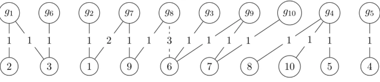
_i

. Example Throughout this and the next section, we illustrate the argument with

the example in Figure

1. There are 10 agents and 15 edges in

F . The edges in F are depicted by solid edges with the u

_ij

values indicated; all these are 1 except for u

₁₇

= 2. The picture does not include the edges in E \ F except for one example:

the dashed line for (6, g

₈

) with u

₆₈

= 3. There are 5 connected components, containing goods {g

₁

, g

₆

}, {g

₂

, g

₇

, g

₈

}, {g

₃

, g

₉

, g

₁₀

}, {g

₄

}, and {g

₅

}, with p

₆

= p

₁

, p

₇

= p

₈

= 2p

₂

, and p

₃

= p

₉

= p

₁₀

. Thus, Θ

₁

= 2, Θ

₂

= 5, Θ

₃

= 3, Θ

₄

= 1, Θ

₅

= 1, and γ

₁

= 2, γ

₂

= 3, γ

₃

= 3, γ

₄

= 1, γ

₅

= 1.

6.1 Constructing the LP

The variables (p

i

)

_i∈[t]

uniquely determine the price of every good. We can formulate the problem of

computing Ψ(F ) in terms of these variables. To differentiate between this t-dimensional price vector

and the n-dimensional price vector of all goods, we say that for a price vector p ¯ ∈

R^t

, the vector p ∈

Rⁿ

is the extension of p, if ¯ p

_ℓ

= θ

_ρ(ℓ)ℓ

p ¯

_ρ(ℓ)

for all ℓ ∈ [n] (in particular, p

_ℓ

= ¯ p

_ℓ

for ℓ ∈ [t]). We also say

that the F -allocation (p, f ) is an extension of p, if ¯ p is the extension of p. ¯

g

₁

g

₆

g

₂

g

₇

g

₈

g

₃

g

₉

g

₁₀

g

₄

g

₅

2 3 1 9 6 7 8 10 5 4

1 1 1 1 2 1 1 3 1 1 1 1 1 1 1 1

Figure 1: Example problem setting.

We now formulate linear constraints that ensure that a vector p ¯ ∈

R^t

can be extended to an F- allocation (p, f ) with ks(p, f )k

_∞

≤ 1, and supp(f ) ⊆ F . The first set of constraints will enforce that all edges in F are MBB, and the second set will guarantee the existence of a desired money flow f with the surplus bounds.

First, the edges in F are MBB if and only if u

_kj

/p

j

≤ u

_kj^′

/p

_j^′

for any k ∈ A, and any g

j

, g

_j^′

∈ G such that (k, g

_j

) ∈ E, (k, g

_j^′

) ∈ F . The θ

_iℓ

coefficients already capture that equality holds if (k, g

_j

), (k, g

_j^′

) ∈ F . For the rest of the pairs, we can express this constraint in terms of the p ¯ variables as

u

_kj

θ

_ρ(j^′_)j^′

p ¯

_ρ(j^′₎

− u

_kj^′

θ

_ρ(j)j

p ¯

_ρ(j)

≤ 0 ∀k, j, j

^′

∈ A, (k, g

_j

) ∈ E \ F, (k, g

_j^′

) ∈ F. (7) We add a second set of constraints for ks(p, f )k

∞

≤ 1. Since f is supported on F and is allowed to be negative, this can be guaranteed if and only if for any component C

_i

, i ∈ [t], the total price of the goods in C

_i

∩ G exceeds the total budget of the agents in C

_i

∩ A by at most γ

_i

= |C

_i

∩ G|. Recall that given the prices p ¯ of the fixed goods, the total price of goods in C

_i

∩ G is Θ

_i

p ¯

_i

. We obtain the constraints

Θ

_i

p ¯

_i

−

X

k∈Ci∩A

θ

_ρ(k)k

p ¯

_ρ(k)

≤ γ

_i

∀i ∈ [t]. (8)

Let us now define the following LP:

max

t

X

i=1

¯ p

i

s. t. constraint sets (7) and (8),

¯ p ≥ 0.

(P

_F

)

Note that p ¯ = 0 is a feasible solution. Using LP duality, the above program is unbounded if and only if the next LP has a feasible solution p ¯ 6= 0.

constraint set (7), Θ

_i

p ¯

_i

−

X

k∈Ci∩A

θ

_ρ(k)k

p ¯

_ρ(k)

≤ 0 ∀i ∈ [t]

¯ p ≥ 0.

(P

_F⁰

)

Example Let us show the formulation for the example in Figure

1. The variables

are p ¯

₁

, p ¯

₂

, p ¯

₃

, p ¯

₄

, and p ¯

₅

. From the constraint set (7), we only show the example of k = 6, j = 8, and j

^′

= 3:

3¯ p

3

− 2¯ p

2

≤ 0.

For the components, we have

2¯ p

₁

− p ¯

₂

− p ¯

₃

≤ 2 5¯ p

₂

− p ¯

₁

− p ¯

₃

≤ 3 3¯ p

3

− p ¯

1

− 2¯ p

2

≤ 3

¯

p

₄

− 2¯ p

₂

− p ¯

₃

− p ¯

₅

≤ 1

¯

p

₅

− p ¯

₄

≤ 1.