ARTICLE
Exploring the Limits of PDR-based Indoor Localisation Systems under Realistic Conditions
Robert Jackermeier and Bernd Ludwig
Chair for Information Science, University of Regensburg, Regensburg, Germany
ARTICLE HISTORY Compiled September 20, 2018
ABSTRACT
Pedestrian Dead Reckoning (PDR) plays an important role in many (hybrid) in- door positioning systems since it enables frequent, granular position updates. How- ever, the accumulation of errors creates a need for external error correction. In this work, we explore the limits of PDR under realistic conditions using our graph-based system as an example. For this purpose, we collect sensor data while the user per- forms an actual navigation task using a navigation application on a smartphone. To assess the localisation performance, we introduce a task-oriented metric based on the idea of landmark navigation: instead of specifying the error metrically, we mea- sure the ability to determine the correct segment of an indoor route, which in turn enables the navigation system to give correct instructions. We conduct offline simu- lations with the collected data in order to identify situations where position tracking fails and explore different options how to mitigate the issues, e.g. through detection of special features along the user’s path or through additional sensors. Our results show that the magnetic compass is often unreliable under realistic conditions and that resetting the position at strategically chosen decision points significantly im- proves positioning accuracy.
KEYWORDS
Pedestrian Navigation, Indoor User Localisation, Inertial Navigation, Map-Matching
1. Introduction
Indoor positioning for pedestrian navigation is still an open problem as no positioning system that delivers absolute – such as GPS – coordinates is available. Many solu- tions providing precise (sub meter) localisation require additional technical devices (Guo et al. 2015; Pham and Suh 2016; Romanovas et al. 2013). However, they are not at disposal in everyday life situations at which pedestrian navigation systems target.
Technically simpler solutions use sensors that come with every smartphone, such as accelerometers, gyroscopes, and step counters (Basso, Frigo, and Giorgi 2015; Verma et al. 2016). Such approaches provide relative positioning data, and often suffer from cold start problems (Harle 2013). In the remainder of this section, we discuss system- atic issues that limit the capability of smartphone sensors to reliably estimate indoor positions even after a series of sensor updates. Furthermore, we identify the fact that
CONTACT Robert Jackermeier. Email: robert.jackermeier@ur.de
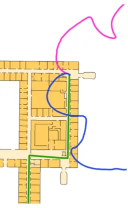
(a) Step trajectories (magenta and blue) influ- enced by magnetic field bias. Actual route in green.
(b) Step length errors often lead to missed cor- ners. Red pluses denote position updates in the wrong area.
Figure 1. Different types of bias that limit indoor positioning.
users – as opposed to technical devices that navigate autonomously in physical spaces – have to cooperate with a navigation system and thereby perform activities that can- not be observed directly as a source for noisy indoor positioning.
1.1. Limits of PDR-based Indoor Localisation
As will be detailed in Sec. 2, it is common to apply inertial sensors to localise users in smartphone-based navigation systems for everyday usage. Unfortunately, magnetic and electrostatic fields cause noisy data and thereby limit the quality of measurements.
The graphic in Fig. 1(a) illustrates the limit caused by magnetic bias. The graphic shows two extreme logs: although in both cases the test person walked on the green line, the smartphone’s orientation sensor computes wrong data from which the actual orientation of the test person cannot be reconstructed. Furthermore, the geometry of the green line is hardly recognisable.
The graphic in Fig. 1(b) illustrates the limit of step length. The test person walks along the corridor – each step is represented by a red dot. At the corner, the person turns to the right. However, as the smartphone estimated the step length incorrectly, the indoor positioning system assumes the test person to still walk straight on although the turn has already been completed (red pluses).
Solutions based on WiFi receivers can compute absolute coordinates of an area in which a user is located. Therefore, they are useful for observing positions, but fail in tracking a user’s movement precisely (Waqar, Chen, and Vardy 2016). In fact, with a standard smartphone WiFi signal updates are slow and often noisy due to unknown
conditions of the physical environment. As a consequence, small movements of a walk- ing person are hard to detect reliably. Detecting large movements only leads to a huge lag in tracking movements as illustrated in Fig. 3(b) (see the yellow line). Further typ- ical types of movements a walking person performs regularly such as turning around a corner cannot be observed directly as the physical principle of estimating positions using radio signals does not allow for it.
Combining sensors for movement and position could – in conclusion – improve the quality of indoor positioning. In fact, as the green line in Fig. 3(b) indicates, this is true, but only to a certain degree. The limit of delay still prevents higher accuracy.
In buildings with many corners, this limit may pose an additional problem to any positioning algorithm: In the context of pedestrian navigation we are investigating in this paper, unreliable position data leads to ambiguous interpretations. Navigation systems assist users to walk along a route calculated earlier and runs into trouble if position data is uncertain resulting in high probabilities that the system assumes users to take paths they actually have not taken.
From such misinterpretations, severe confusions may arise that are well-known even in outdoor areas. Using a navigation system as a pedestrian in a historic city cen- tre is often frustrating as the system receives wrong or even no GPS updates and in consequence locates users at wrong positions and computes erroneous navigation instructions that users are unable to understand.
Given this situation, we are convinced that – even if in the last years many re- searchers worked on this topic – it is still worth new research efforts. Actually, they seem even to be mandatory for building indoor navigation systems that can provide reliable assistance to their users.
1.2. Tracking Activities of Pedestrians
Experience gained in the last years shows that – due to the limits described above – in- creasing the accuracy of state-of-the-art indoor positioning algorithms for smartphone users (which we focus on in this paper) with more data only will hardly result in suf- ficiently small error rates. Although – as Waqar, Chen, and Vardy (2016) point out – the mentioned state-of-the-art approaches can advantageously be used to implement indoor positioning rapidly at any location that provides the necessary infrastructure, more context information is necessary to overcome the limits described above.
For navigation systems, such context information can be derived from the calculated path to a target and the activities that persons have to perform in order to reach the target. In fact, it is just these activities that have to be observed – either directly or indirectly by calculating a sequence of position estimates.
We address exactly this issue and describe an approach that models spatial knowl- edge for routes with an indoor navigation graph (see Fig. 2 as an example). The graph contains all routing decisions and path segments between any two arbitrary locations in an indoor/outdoor environment. Our algorithm for tracking the activities of pedes- trians snaps position updates from smartphone sensors to particular edges of the graph while they are navigated along a route calculated in advance. Position updates are computed using PDR based on a Step and Heading System (SHS) approach. Typical activities of pedestrians are:
• walking straight ahead
• turning left/right
• walking upstairs/downstairs
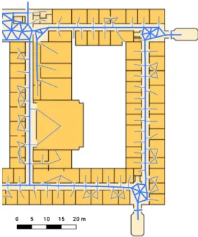
0 5 10 15 20 m
Figure 2. Indoor navigation graph in one of the test areas. Main edges used for localisation are shown as thick lines. Notice the mesh-like topology in larger open areas.
• going up/down in an elevator
• taking an escalator uphill/downhill
In this work, we explore to what degree the activities ofwalking straight ahead,turning left, and turning right can be observed with a standard SHS approach. We identify situations of different accuracy rates and argue that each activity needs a particular classifier in order to increase the overall accuracy of indoor positioning.
1.3. Tracking Pedestrians on a Navigation Route
In order to observe activities with a standard SHS approach we map each activity on the area that has to be traversed in order to complete it. In other words, to each activity during a navigation task, there exists
(1) a corresponding navigation instruction and (2) an area in which the activity takes place.
Therefore, we segment a complete route according to the navigation instructions cal- culated by the route planner of our system into a single area for each instruction and observe the corresponding activity by mapping position updates onto the area. In or- der to be able to evaluate the success of the approach, we introduce thearea match scoreas a new metric for indoor positioning: we calculate the probability of a posi- tion update to fall into the area corresponding to the area for the current navigation instruction. In this way, we establish a task-based concept of context for indoor posi- tioning that has the potential to overcome the limits described above.
For the evaluation, we have collected a large corpus of indoor data under realistic conditions: test persons had to walk on routes of roughly 800 m containing all types of activities several times and show quite different architectural characteristics. There- fore, the routes are typical for real world applications and avoid memory biases that could influence the walking (and information) behaviour of the test persons.
From results of the analysis, we conclude that effective positioning algorithms for pedestrian navigation must be able to apply different techniques for sensing the user’s environment in order to correctly track the user activities during a navigation process.
1.4. Structure of the Paper
In this paper, we first report the relevant state of the art, then we explain how we re- late landmark-based navigation and indoor positioning and develop our mathematical model for the posed problem. Next, we present three empirical evaluations for navi- gation tasks that required test persons to walk on indoor routes of varying complex- ity across several buildings on the campus of our university. Finally, we discuss the obtained results in the light of our task-based performance metric. We analyse lim- itations of the approach and derive relevant issues of future work from the insights obtained from the evaluation.
2. State of the Art in Indoor Positioning
As already mentioned, many localisation techniques based on different types of sensors have been proposed for pedestrian indoor navigation systems and indoor positioning in a broader sense. Despite all these research efforts, there is still no technology es- tablished as a widely accepted state of the art similarly to GPS for outdoor areas. In particular, published research results – the most recent ones (e.g. from the last IPIN conference) will be discussed below – are based on data collected in short-distance and short-time experiments and therefore do not reflect typical characteristics of realistic indoor applications such as trying to reach a target in large buildings such as airports or train stations, visiting a museum, or searching an office in a multi-level building.
Therefore, in order to build up a corpus containing more complex data we conducted a series of experiments that will be described in detail in a later section.
As our work is focused on positioning algorithms that assist users in everyday nav- igation tasks and may not need sensors beyond those available in a standard smart- phone, the following review of the state of the art on PDR leaves aside more exotic approaches that require special sensors or hardware.
WiFi-based indoor localisation can be widely deployed in modern buildings where a sufficient WiFi infrastructure is usually available, but suffers from multiple problems, as Davidson and Pich´e (2016) point out: Creation and maintenance of radio maps is time consuming and therefore expensive. A low scan rate on current smartphones leads to disjointed position estimates. Furthermore, device heterogeneity, influence of the smartphone’s orientation, and the attenuation of signals by humans are identified as disadvantages. Due to these issues, WiFi-based systems generally achieve an accuracy of at most a few meters and are suited to determine the approximate position, but not for continuous tracking.
Our own findings confirm these claims: Figure 3(a) shows some of the results from an earlier study, where the location reported by Fraunhofer’s WiFi-based awiloc system1is wandering around in an indoor area even if the test person is not moving. Consequently, the RMSE of the position reaches up to 5 meters. Even more problems arise when the test person is moving (an example can be seen in Fig. 3(b)), where the location updates usually are lagging behind and do not match the path that was actually taken.
1https://www.iis.fraunhofer.de/en/ff/lv/lok/tech/feldstaerke/rssi/tl.html
0 2.5 5 7.5 10 m
(a) Result of a previous WiFi study in an indoor area using Fraunhofer’s awiloc. While standing still at the po- sitions indicated in red, the reported locations (coloured dots) are scattered around the area with a root mean square error between 2.1 and 5.0 m.
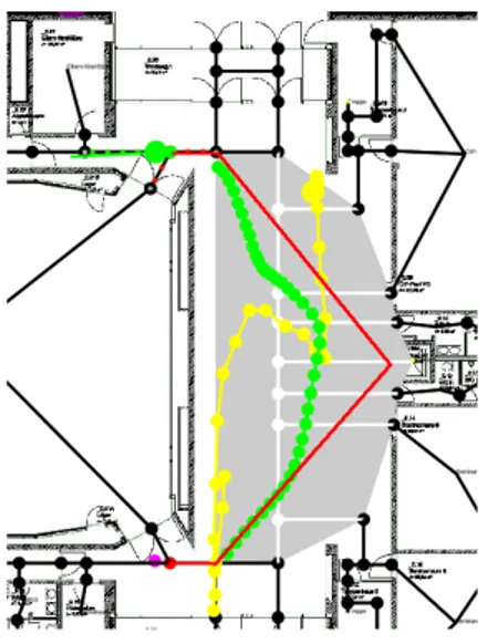
(b) Result of a previous WiFi study in an indoor area using Fraunhofer’s aw- iloc. The position reported by awiloc (yellow) follows the ground truth (red, from bottom to top) very loosely, if at all. Only by fusing step detection data with a Kalman filter (green) the actual trajectory can be approximated.
Figure 3. Performance of WiFi signals in indoor positioning tasks.
On the other hand, Bluetooth Low Energy (BLE) beacons as another wireless lo- calisation technique are designed to be more accurate, but are far less widespread and therefore more expensive to deploy. In particular, as they are mounted at fixed posi- tions and send signals over a small distance only, persons could be tracked continuously only if beacons were mounted along all paths persons can walk on.
A recent development for getting an rough estimate of the user’s position bases on sending a sound signal via the smartphone’s loudspeaker and recording it immedi- ately with the microphone. Rooms have particular acoustic characteristics that can be recognised to identify in which room out of a set of trained rooms the smartphone is currently located (see Rossi et al. 2013).
Both BLE and acoustic approaches are examples for zone-based localisation ap- proaches: their aim is to identify positions in a rough approximation of an existing physical space instead of tracking user activities as we intend to do. To the best of our knowledge, there is no evidence that with these approaches user activities taking place in a very limited space may be observed reliably. For example, while it is possible to detect that a user is positioned in a foyer, it is hard to observe that he is turning right in this foyer in order to reach the door of an elevator. Consequently, zone accuracy as presented e.g. in Pulkkinen and Verwijnen (2015) has to be distinguished from our area match score: while for zone accuracy it is sufficient to locate the user in a certain zone, for the area match score, the same observation is necessary, but not sufficient as e.g. a right turn in the foyer, and in particular in front of the elevator door has to be detected if this activity is currently expected by the navigation system to continue on a computed route. Additionally, we want to note that the turn to the right may be detected by other approaches than computing a sequence of several small position changes and then reconstructing the turn from some kind of interpolation of the posi-
tion updates. For example, the accelerometer of the smartphone could help to detect a rotation that is expected for a turn.
In summary, several approaches exist that provide a rough estimate of the user’s cur- rent position, but not of the user’s movement. A notable exception for moving up/down is the SemanticSLAM algorithm described in Abdelnasser et al. (2016). However, users also perform other activities. For their recognition in a hybrid approach, correspon- dences between activities, positions, and areas can be exploited to collect redundant data reliably. Later in this paper, we will provide empirical evidence that redundant data is actually necessary as data of a single sensor often leads to ambiguous interpre- tations (see the discussion in Sec. 1.1).
Still the most important approach for PDR is a variant of so-called Step and Head- ing Systems, that detect the user’s steps and try to estimate their length and direction (Harle 2013). Step detection on smartphones is historically achieved through the ac- celerometer using various techniques (see Susi, Renaudin, and Lachapelle 2013; Muro- de-la Herran, Garcia-Zapirain, and Mendez-Zorrilla 2014; Sprager and Juric 2015).
Lately, dedicated step detector sensors are available in more and more devices. The heading can be inferred from the magnetic compass and gyroscope of smartphones, while step lengths can be either assumed as fixed or dynamic, e.g. based on the fre- quency (Harle 2013).
A further limit of PDR is the need for an initial position from which the relative positioning can start as SHS by their nature cannot compute absolute positions. Fur- thermore, the positioning error increases over time due to noisy sensor data. Given both of these problems either error correction through external sensors or an algorithm that matches the sensor data to a final position estimate are necessary to employ dead reckoning for more complex tasks such a navigating a user or other location-based ser- vices.
As in our work external sensors should be avoided, matching algorithms that pro- vide context information are the only option to address the PDR limits. Context information is often provided in terms of maps, which in turn are often represented as discrete graphs (see e.g. Thrun, Burgard, and Fox 2005) and have been used suc- cessfully to locate robots in complex environments. For pedestrian indoor localisation, graph models of the environment were first introduced by Liao et al. (2003) in com- bination with the particle filtering method in order to make position estimation more robust and efficient. Since then, other researchers have adapted and improved this ap- proach (e.g. by adding multiple sensor modalities): the system recently presented by Hilsenbeck et al. (2014) is operating on a graph generated from a 3D model of the environment. Herrera et al. (2014) use existing material from OpenStreetMap and en- rich it with information about the indoor areas of a building. A similar approach is taken by Link et al. (2013), who use sequence alignment algorithms to match detected steps with the expected route. Ebner et al. (2015) generate a densely connected graph from the floor plan of a building. All these approaches have in common that creating a map is either time consuming or expensive (due to the need for special hardware) or relies on existing data. Furthermore, normally the resulting graphs do not contain any information besides the geometry of the building, making them unsuitable to use as data source for the path planner of a navigation system.
In our approach instead, we use graphs that represent all activities a user can perform in a given physical environment and contain information where these activities can be executed. The main advantage is – as already outlined in the discussion of BLE above – that we now can observe activities indirectly by reconstructing them from position updates – thereby reducing the impact of noise –, or directly by other sensing
strategies, or using hybrid approaches that fuse data from several sources.
Particle filtering has become the de facto standard for hybrid localisation systems that combine PDR and additional sensors, with many improvements proposed since its introduction. Most prominent among them is the Backtracking Particle Filter (Klepal, Beauregard et al. 2008; Beauregard, Klepal et al. 2008), which is particularly suited to generate smooth and coherent trajectories when calculations can be performed offline, but provides little or even no advantage in real-time scenarios. It does however serve as an example for map-matching that is not based on a graph structure, but on the actual floor plans. Compared to the graph-based systems described above, the environment can be represented more faithfully, with the downside of higher computational cost.
As far as the evaluation of indoor positioning is concerned, the state of the art can be surveyed best by looking at recent competitions that aim to compare the performance of indoor positioning systems. Held regularly, they provide an opportunity to gain insights into established evaluation methods. Potort`ı et al. (2015) report the results of the EvAAL-ETRI competition held in conjunction with the IPIN 2015 conference. To assess the error of the participating systems, they add a penalty for wrongly detected floors or buildings to the actual positioning error. The final ranking is determined by the 75% quantile of the resulting errors. In their evaluation of the 2015 EvAAL-ETRI WiFi fingerprinting competition, Torres-Sospedra et al. (2017a) rank the competitors by the mean positioning error, which is also used by Lymberopoulos et al. (2015) for the participants of the 2014 Microsoft Indoor Localization Challenge. Interestingly however, they remark that the mean error or other commonly used metrics do not represent the performance of a system in its entirety. We follow this assessment and argue for a task-oriented view on the performance of a positioning approach that we introduce below.
Sensor data for the IPIN 2016 offline competition was collected by an actor walking along a predefined path as closely as possible, stopping at certain points to mark the ground truth (Torres-Sospedra et al. 2017b). For the offline competition at IPIN 2017, a few variations of carrying the device, e.g. by simulating a phone call, were added (Torres-Sospedra et al. 2018). In recent Microsoft Indoor Localization Challenges, only static locations were evaluated (Lymberopoulos and Liu 2017).
To our knowledge, none of the existing studies actually create a realistic scenario for the intended application context, i.e. in our specific case a navigation task in an area that is (at least partially) unfamiliar to the test person. The methodology presented by De La Osa et al. (2016) aims at real-life use cases, but still relies on a tester who can identify checkpoints on a predefined path.
3. Landmark-based Navigation
In the following section, we give an overview of the navigation system we use in the experiments that we discuss later in the paper. In particular, we describe how the graph model relates to areas and corresponding activities of indoor routes. Based on this description, we then introduce the particle filter implementation that forms the core of our indoor positioning approach.
3.1. Data Model
Fig. 2 visualises our data model that we callindoor navigation graph. It is used for com- puting routes, generating navigation instructions, and indoor positioning (see M¨uller
et al. 2017 for details). In order to be able to serve these three purposes, it formalises knowledge about activities pedestrians perform in the physical environment. All pos- sible activities (see Sect. 1.2) are represented as edges in the graph, while the nodes represent locations where these activities can take place. In particular, source nodes of edges represent the location where an activity can start, and sink nodes are used for the location pedestrians are expected to reach after they have completed the activity successfully. The edge is typed by a unique activity out of the list above and indicates which kind of movement is to be expected next. In this way, we could potentially train classifiers for each edge type.
Furthermore, the graph contains nodes for objects pedestrians can observe in the environment (so-called landmarks). They are used to segment a route into areas. One navigation instruction is computed for each area. While navigating a user, the system has to keep track whether the user has completed the current activity as requested in the current navigation instruction. Following this approach, for locating the user it is sufficient to know that the user is close to a landmark (e.g. a door at the end of a corridor or a certain cloth shop in a shopping mall) as human users are capable to approach the landmark autonomously, i.e. a pedestrian can walk to a distant object without continuous technical assistance while a robot cannot. Therefore, the mean positioning error – while being definitely of interest for building autonomous systems that can navigate in indoor environments (e.g. robots for ambient assisted living) – for the implementation of many location-based services it is an inappropriate performance metric. Consequently, the precision of indoor positioning for pedestrian navigation systems should be measured in terms of the degree to which the current task-related activity is completed instead of in meters in a coordinate system that the user cannot even perceive (see e.g. Ohm, M¨uller, and Ludwig 2015).
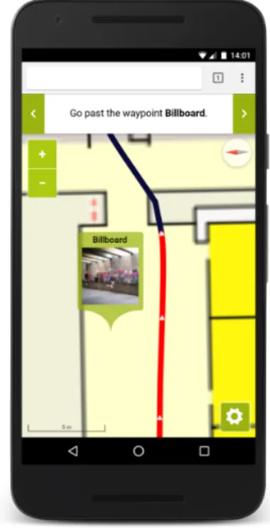
At this point, we can state one major contribution of the present paper. We pro- pose an approach to combine a graph-like representation of an environment with the minimally necessary metric information to correctly align the data computed by a SHS in the graph in order to assign the user’s position to more easily perceivable objects in the environment which we callareasorlandmarks depending on whether we refer to a part of a path the user should walk on or a relevant object the user can perceive in the environment. An example can be seen in Figure 4, which shows part of a corridor as an area consisting of a several adjacent edges. In Figure 5 a typical landmark is displayed: the billboard shown on the map is also referred to in the navi- gation instruction. This approach for an indoor navigation system shares similarities with other work (in particular Link et al. 2013). As a new contribution, we introduce the concepts ofareas and thearea match score that link indoor positioning based on SHS with landmark-based navigation (see Sect. 3.2). By doing this, we relax per- formance requirements for positioning algorithms as we no longer need to optimise the metric errors at any time of the navigation process. Instead, it is sufficient to iden- tify the correct area a user is currently walking on: given the current area, the system can generate a navigation instruction that incorporates a landmark easily perceivable from the estimated position of the user.
In a similar fashion, Pulkkinen and Verwijnen (2015) remark that for certain appli- cations it is more important to reliably identify the room where a person or object is located than to know the exact position. They therefore introduce zone/cell accuracy, operationalised e.g. as the classification error. Our approach, in contrast, does not rely on predefined, static zones derived from the building geometry, but generates its areas dynamically depending on the planned route and the available landmarks. In other words, our areas are not necessarily tied to the building layout but rather temporarily
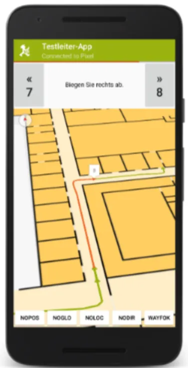
Figure 4. User interface of the data collection app for the initial study. The current area is highlighted in light red.
Figure 5. Example of a landmark- based navigation instruction.
partition the space in a way that relates to the current navigation task.
As stated above, for landmark-based navigation it is crucial to give navigation instructions at the right time in order not to confuse users and to guarantee good usability as well as reaching the destination. A navigation instruction is given at the right time if it does not refer to any landmark that is not yet visible from the user’s current position or that the user has already passed. As a consequence, for indoor positioning the main difference to zone accuracy lies in the fact that the positioning algorithm has to determine whether the user iscloseto the landmark and can switch to the next instruction. Mostly, this task is much easier than continuously determining the exact position.
For the effort to create indoor navigation graphs, we note that it is impossible to extract all the information about decision points and likely taken paths algorithmically, especially when working with imprecise or outdated plans. The data we need goes beyond what is contained in automatically generated topological building models (e.g.
Hilsenbeck et al. 2014). While there is no doubt that the automatic generation of models for indoor environments will see much progress in the future – in particular due to the application of modern machine learning techniques –, this issue is not in the focus of our work. Instead, by entering the information intellectually and – if needed – on-site, we can achieve a higher similarity between model geometry and actual trajectory. In summary, the system relies on a single data model for routing, instruction generation, and localisation that allows us to minimise the effort needed for map creation and maintenance.
3.2. Graph-based Localisation
In order to give the correct instructions at any time, the user’s relative position to- wards landmarks referred to in navigation instructions needs to be known. Our indoor positioning algorithm computes this position by mapping sensor data to areas in the indoor navigation graph. For this mapping, we implemented a recursive stochastic fil- ter that after each measurement assigns a probability to each area proportional to the likelihood of the user to currently walk on a certain area.
The filter is implemented as a particle filter (see Thrun, Burgard, and Fox 2005).
This family of algorithms represents a probability distribution by means of a represen- tative sample, a set of so called particles. Around the expected position the number of particles is high while elsewhere it is low according to the small probability mass.
Using a sampling and resampling strategy the set of particles is updated after each measurement in order incorporate the new information (see Thrun, Burgard, and Fox 2005 for details): far away from the expected position the particles diminish while new ones are generated for positions with high probability mass. Our implementation can also incorporate input from multiple sensors such as detected steps or WiFi signals in order to implement the advocated hybrid approach for indoor positioning. Further- more, information contained in the indoor navigation graph stabilises and corrects the position estimates as many constraints for the user’s current location can be derived from the graph structure (in particular invalid positions receive probability zero while in standard SHS approaches the same locations are possible positions).
The implementation does not rely on a particular sensor technology or SHS algo- rithm, but only assumes to receive vectors that quantify the step length and direction of a pedestrian’s movement. In fact, we do not perform any low-level sensor fusion or step detection based on raw sensor values. In order to investigate the influence of the precision of the SHS on our approach, we compared two different algorithms:
• motionDNA by Navisens
The motionDNA SDK by Navisens is a well-known commercial state-of-the-art motion tracking solution. According to the company’s website2, it relies on iner- tial sensors only and does not need any external infrastructure to operate. The sensor readings are updated with a rate of 24 Hz on our test device and include a variety of information such as the user’s activity and the device orientation and position. For this study, only the position information (relative to the initial position, measured in meters in X and Y direction) is used.
• Android’s built-in sensors
On recent devices, the Android framework gives access to many sensors that can be used for motion tracking. The step detection sensor tells us whenever a step occurs. Since it does not provide a step length, we initially use a fixed length and later use the particle filter to adapt to the user. Under the assumption that the user orients the smartphone roughly in his walking direction, the average orientation during the step as provided by the rotation vector sensor is used as step direction. Though this may seem like a strong assumption, we show empirical evidence later on that in the targeted scenario pedestrians tend to carry their device in exactly that way most of the time.
In Fig. 6 the data computed by each of both algorithms for a single walk on the test route of the initial study is plotted into the map of the building. Many position
2https://navisens.com
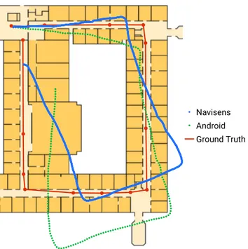
Navisens Android Ground Truth
Figure 6. The trajectories of both motionDNA (blue) and raw step data (green) of a typical walk along the test route of the initial study. Ground truth (starting top left, then clockwise) and the boundaries of the areas defined for the evaluation experiment are drawn in red.
estimates are far off the route. This observation illustrates that information about the environment is indispensable for the position estimates to be used in an indoor navigation system.
In order to map SHS estimates to the indoor navigation graph, we apply the de- scribed particle filter. Initially, the probability is distributed uniformly over all edges.
If information about the start position is available, e. g. during a navigation task, we use a normal distribution centred around the start node instead to sample the initial particle set.
Whenever a step is detected, a Gaussian naive Bayesian classifier updates the prob- ability distribution for the edges starting in the current node. The update takes the motion model for the user (i.e. the distance and direction of the detected step) and the orientation of the considered edges into account. The probability of the user to walk on an edge increases if this edge is parallel to the direction detected by the SHS.
The increment for an edge not parallel to the detected direction decreases proportion- ally to the angle between the direction and the orientation of the edge.
Unlike other approaches, the algorithm does not immediately select the edge with the highest probability as the current position estimate. Instead, it updates the set of particles each of which represents a different hypothesis for the user’s current position.
A similar approach has been successfully applied to localisation in robotics (see Thrun, Burgard, and Fox 2005) and allows to
• account for noise in the SHS data, which may stem from the rotation vector sensor (or rather the underlying magnetic compass) or the way the device is held in the hand,
• account for differences in step length while a person is walking, and
• account for different step lengths of different users.
More formally, each particle’s state is defined by the vector {nt, dt, et}, where nt de-
notes the starting node at timet,dtthe distance walked since leaving the node, andet
a discrete probability distribution for the edges adjacent to the node. On every step, the state is updated according to
{nt, dt, et} ∼p(nt, dt, et|nt−1, dt−1, et−1, zθ,t, zl,t, G), (1) wherezθ,t andzl,t are the measured step direction and length, andGis a indoor navi- gation graph. Applying the procedure detailed in Hilsenbeck et al. (2014), the update rule can be decomposed to its independent parts. The noisy step length measurement with the empirically determined varianceσl2 is modelled by
lt∼p(lt|zl,t)∼ N(zl,t, σ2l), (2) leading to the updated cumulative step distance of
dt∼dt−1+lt. (3)
Similarly, the step direction is updated by
θt∼p(θt|zθ,t)∼ N(zθ,t, σθ2) (4) and subsequently used to determine the new edge distribution:
eit∼p(eit|eit−1, θt, G)∼ N(∆θti, σe2)∗eit−1 (5) Here,eitdenotes the probability of the user to currently walk on thei-th edge adjacent to the current node and ∆θti the angle difference between the step and the i-th edge.
Finally, the decision whether the user has completed an edge and moved to the next is formalised as:
nt∼ (
no ifdt≤length(e)∧e= argmaxi(et)
yes ifdt>length(e)∧e= argmaxi(et), (6) i. e. wheneverdtexceeds the length of the currently most probable edgee. In this case the starting node has to be updated: nt is set to the sink node of the previous edge and dt is reset to zero. Since the walked distance usually does not align exactly with the edge length, the difference is added to the position estimate and the step bias is reinitialised toN(zl,t, σl2) as the prior distribution for the new current edgeet.
After the update step, the particle importance weights are distributed according to the non-normalised probability of the most probable of all adjacent edges:
ωt=ωt−1∗p(zl,t, zθ,t|nt)∼ωt−1∗max
i (et) (7)
Finally, stochastic universal sampling is performed, which guarantees low variance and a representation of the samples in the new particle distribution that is proportional to their importance weights (see Thrun, Burgard, and Fox 2005 for further details).
In order to estimate the user’s position, the expected value of the particle distribu- tion is calculated. From there, the closest point that is located on either an edge or a node of the graph is computed as the final position estimate. This snap to the indoor
navigation graph ensures that the position estimate is a location that is accessible to the user and – differently to the pure SHS algorithms – prevents the positioning algo- rithm to assume impossible movements, e.g. through walls.
4. Task-Oriented Evaluation
As stated above, a central objective of our work is to observe the activities of users in the context of navigation tasks. As these activities correspond to certain traces of movements that can be observed by state-of-the-art sensors, we can exploit this dualism for activity recognition. In practice however, as we also noted above, the state of the art of tracking movements is still imperfect. One reason for this – and therefore a chance for improving the accuracy – may be the fact that currently for indoor positioning all existing approaches use one single algorithm even if the physical models underlying the different kinds of movements actually suggest that for each kind of movement a particularly suited algorithm could be appropriate. While this observation is obvious for walking upstairs compared to walking straight ahead in a plain space, in indoor positioning a distinction has never been made e.g. between classifying raw data intowalking straight aheadandturning right. However, as research in biology and medical engineering suggests (see Novak et al. 2014; Nandikolla et al.
2017; Hase and Stein 1999; Sreenivasa et al. 2008), it could well be worth to train a different classifier for each type of movement.
As a first step in this direction, we wanted to analyse realistic data whether posi- tioning errors of a state of the art-SHS-approach can be better explained if one knows the expected type of movement. It could, for example, to true that on average SHS- approaches perform well if users walk straight ahead, but could fail quite often to detect users to turn aside.
Therefore, in order to explain the limits of PDR-based indoor positioning systems, we have conducted three studies so far. In this section, we will describe each of them in detail and reveal typical situation in which the accuracy of indoor positioning is low.
The first study introduces the concept of task-oriented evaluation and the area match score, while in the second experiment we collected and analysed data under realistic conditions for everyday navigation scenarios. In the third study, we collected and evaluated new data, taking the lessons learned from the previous studies into account.
4.1. Study 1: Applying the Area Match Score
The purpose of the initial study is to demonstrate the benefits of a task-oriented performance metric that shows how well the correct area on a route can be determined by the localisation system, which – as noted above – is a requirement for correct navigation instructions and for successful navigation in general. From the pedestrian’s perspective, the concept of area-wise navigation instructions and the area match as an estimate of the pedestrian’s performance result in minimising the cognitive workload necessary for aided wayfinding.
The second purpose of this study is to identify contexts and situations during a navigation task that point to problematic areas and to propose ways to mitigate the revealed issues.
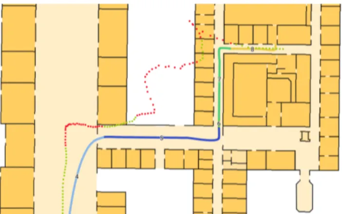
Figure 7. Detailed view of the results for a single walk on the second half of route 1 of study 3. Green dots denote successful position estimates; red dots represent estimates that are located in the wrong area or too far away from the route.
4.1.1. Setup
Based on the mathematical model introduced in Sect. 3.2, after each sensor data update t our indoor positioning algorithm predicts the user’s current position pt. If and only if the distance betweenptand the spline interpolating all nodes of the current area is sufficiently small,ptmatches this area (see Fig. 7). The user is now assumed to execute the activity corresponding to the calculated area. For this choice to be perfect, i.e. to be always correct, users have to walk exactly on the spline, and the sensor data has to precisely observe this movement.
To collect data for an evaluation of the implemented indoor positioning algorithm, we conducted an empirical study in the ground floor in an university building. There, we defined a test route spanning 182 meters. The route leads through 4 corridors in a rectangular shape. Three of the corners are modelled as small foyers (see Fig. 2). The only obstacles on the route are several glass doors that had to be passed in order to reach the destination of the route.
The route was segmented into areas as described in Sect. 1.3. Their boundaries were set at positions where semantically relevant objects – i.e. salient landmarks – are located. For determining salient landmarks along the route, we followed the approach described in Kattenbeck (2016): 19 persons rated 32 objects in the test area regarding different aspects of their salience. We selected the objects with the highest predicted overall salience as landmarks for the navigation instructions in our experiment. These landmarks included e.g. a glass cabinet, a wall painting, a bench and a sign for the department of psychology. Additionally, architectural features such as the aforemen- tioned glass doors or the beginning and end of foyers were used to segment the route into areas. For each area, we formulated a navigation instruction that should explain to the test persons how to proceed the route. Finally, the route consisted of fourteen areas of varying size (see Fig. 6). The main factor that influences the size of the areas is the visibility of the landmark at their end: some can be referenced unambiguously from further away, while for others one has to be closer, thus causing smaller areas.
4.1.2. Procedure
Acquisition of Positioning Data
Starting from a defined position, 7 different persons who were familiar with the area
and the landmarks performed a total of 15 walks along the test route. Data collection took place over the course of several days, with an LG Nexus 5X running Android 7.1.2 as the test device. Before each test run, the compass was calibrated and its proper functionality was verified. During the experiment, the phone was held in the hand in front of the body, pointing in the direction the person was heading toward.
For data collection, a custom Android application was developed. It is able to cap- ture data from various sensors of the device:
• Steps detected by the built-in Android step detection sensor.
• Orientation data from Android’s rotation vector sensor, which in turn fuses mag- netometer, accelerometer and gyroscope readings.
• Data from Navisens’ motionDNA SDK. First and foremost, this includes the relative position, but also heading direction, orientation of the device, as well as detected user activity.
• The signal strength of nearby WiFi access points (not used in this study).
• A video recording of the device’s back-facing camera, capturing the test person’s feet and the area immediately in front of them.
The app’s user interface consists of a map of the test area and a single button that allows the user to start the test run. At the beginning of each test run, the indoor positioning system is initialised on the starting node of the test route. Next, the first area to traverse is highlighted on the map and the corresponding navigation instruction is displayed. Each time a test person reaches the landmark related to the instruction, he or she has to press the button in order to set the ground truth for the transition between two adjacent areas. Finally, the interface is updated with information for the next area on the route. This procedure is repeated for each area of the chosen route.
Validation of the Collected Data
With this experimental setup, we collected sensor data for the test route and a ground truth labelled by experts in a single run of the experiment. As all test persons were instructed before the experiments how to label the ground truth, the data sample is valid for mathematical analyses.
In order to verify whether the collected samples were representative for average persons walking straight ahead, several gait characteristics were calculated:
• The mean gait speed during a walk can easily be determined by the quotient of route length and the time needed to complete the route, measured by the difference of timestamps between last and first step. The result is a mean speed of 1.30 m/s (SD = 0.14 m/s), which is well within the margin reported by Bohannon and Williams Andrews (2011).
• In order to calculate the step length, the steps are counted manually for each walk by means of the recorded video, revealing that Android’s step detector misses about 5.8% of steps on average.
• The mean step length amounts to 0.73 m (SD = 0.077 m), which is classified as fast gait according to the study from Oberg, Karsznia, and Oberg (1993). This can be explained by the fact that the test persons knew the area and the route very well.
In summary, the collected data is representative for the activities of humans during the pedestrian navigation processes we want to analyse.
4.1.3. Analysis of the Collected Data
The analysis of the raw data shows – quite expectedly – that the error quickly accu- mulates, leading to a high mean location error of 11.5 m (Android sensors) respectively 12.0 m (motionDNA). Figure 6 shows the trajectories of a typical walk. Navisens’
motionDNA often struggles with substantial drift towards the left early on, but other- wise manages to track the overall shape quite well. The version relying on the Android step counter usually shows drifts in different directions throughout the walk due to the lack of correction. Additionally, the reported distances differ between the track- ing methods: motionDNA’s paths are usually shorter (M = 174.1 m, SD= 15.37 m), Android’s longer (M = 189.4 m,SD= 16.49 m) than the ground truth of 182.0 meters.
Before the motionDNA data could be used as input to the particle filter, some preprocessing was inevitable: Since the update frequency of about 20Hz was rather high (about an order of magnitude higher than the step frequency), the data was split in batches of ten measurements that were treated as a single step. In two of the 15 recorded walks, the relative location reported by motionDNA unexpectedly was set back to the starting point of the route. Therefore, the area in which the reset occurred was eliminated from the data set.
4.1.4. Results
Since it was not feasible to run both Navisens’ and our indoor localisation implemen- tation at the same time on one device, we processed the collected data in an offline simulation of our indoor positioning algorithm.
In order to extend the data set, sensor data from each actual walk was used multiple times with different initial random seeds for the particle filter, resulting in 10 iterations for motionDNA and the Android sensors, respectively.
The extended data set was used for the evaluation of the implemented algorithm.
In the remainder of this section, we present our evaluation results and discuss their impact on the appropriateness of the proposed area match score for localising users during indoor navigation.
Accuracy Metrics for the Sensor Data
Figure 8 shows a comparison of the two motion tracking solutions regarding their positioning accuracy, i. e. the distance from estimated position to ground truth, after their raw data has been processed by the particle filter.
The mean and median error of motionDNA amount to 7.02 and 4.28 meters respec- tively, while the Android sensors lead to an accuracy of 4.39 (mean) and 2.60 (median) meters. This performance gap is likely caused by two factors:
• The drift at the beginning that motionDNA often suffers from is propagated throughout the whole walk, causing a mismatch between step directions and the graph edges.
• Open spaces at the ends of the corridors allow for some overshooting, which benefits the approach using Android sensors and its slightly longer steps. The too short distance reported by motionDNA however can often not be compensated by the particle filter.
Analysis of the Area Match Score
On average, 60.6% (motionDNA) resp. 74.7% (Android sensors) of position updates are assigned to the correct area. Figure 9 visualises the area match score for each area
0.00 0.25 0.50 0.75 1.00
0 10 20 30 40 50 60
position error [m]
CDF
Tracking method
Navisens Android sensors
Figure 8. Empirical cumulative distribution function showing the accuracy with the two different motion tracking methods.
on the route. Obviously, the choice of the SHS influences the overall performance of our positioning algorithm. It cannot repair arbitrary errors of the SHS as positions too far away from any edge and directions very different from the orientation of the edges nearby the user’s current position decrease the probability of the particles for these edges significantly (see Eq. 5).
1.00 0.21
0.75 0.39 0.51
0.75
0.72
0.80 0.30 0.29 0.58 0.21
0.59 0.68
1.00 0.68
0.89 0.77 0.82
0.79
0.74
0.95 0.44 0.56 0.78 0.13
0.70 0.80
Navisens Android sensors
0.00 0.25 0.50 0.75
area match1.00
Figure 9. Area match scores for the two motion tracking methods.
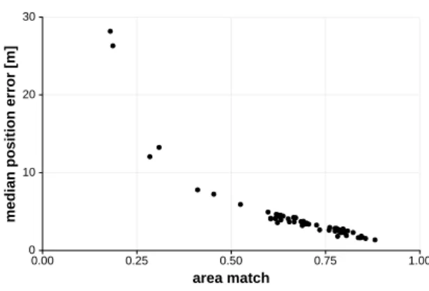
As Fig. 10 illustrates, the area match score and the positioning error are inversely correlated (r(58) = -0.87, p < 0.05). From these observations we conclude that in order to support indoor navigation effectively any indoor positioning needs to be able to reliably estimate a user’s relative movements. While in this study we only analysed walking, this observation in a more general setting equally applies to other kinds of movement (e.g. climbing stairs, taking an elevator, etc.).
Influence of the Navigation Graph on the Area Match Score
While from the preceding analysis we learn the lesson that the area match score’s precision depends on the quality of the step detection, in the following we identify
0 10 20 30
0.00 0.25 0.50 0.75 1.00
area match
median position error [m]
Figure 10. The area match score correlates inversely with the median positioning error. Each point represents the mean of 10 simulated runs for one actual walk.
other sources for area match errors.
The first source is the indoor navigation graph. Its usage introduces artifacts for the actual movement of a person as it always has to be snapped on one of the edges – sometimes a very crude discretisation of the actually available degrees of freedom how to move.
While in corridors no problems may arise, Fig. 9 illustrates that in junctions and foyers, the area match score tends to decrease. The limits ofdelay,magnetic bias, and step length amount to the problem of turn detection. The sensors obviously are not fast enough to reliably reconstruct the pedestrian’s motion – this is a clear hint for the need to develop classifiers for turns as part of future work in indoor positioning.
Such a classifier should take the context (i.e. the activity users are expected to perform according to the current navigation instruction) into account.
By analysing the data and the indoor navigation graph, we revealed a second issue that influences the area match score: junctions of two corridors are often modelled using three edges only (see Fig. 11). In such situations, there is only a single correct edge that can be hypothesised as the current position. However, the particle resampling may fail when the SHS due to the limits mentioned above misses the user’s turn or at least recognises it too late. In this case only few or even no particles are generated for the current edge while the majority of the particles hypothesises the user to continue to walk straight ahead. This phenomenon is particularly obvious for the junction on the bottom left in Fig. 9.
Contrarily, the three other larger foyers are represented by a densely connected net that enables the system to track almost arbitrary paths within these areas (see Fig.
2). In these areas, the area match score remains high.
This circumstance teaches us that indoor navigation graphs should not only model accessibility relations between locations in the modelled environment, but also approx- imate the geometry of the locations.
We tested this hypothesis by connecting the nodes adjacent to junctions with addi- tional slanted edges as depicted in Fig. 11, the benefits of which are twofold: Firstly, it models more natural paths where the test person cuts the corner slightly; secondly, it allows for the compensation of step length differences since now multiple paths lead into the corridor that is branching off.
Using the new graph structure, we repeated the computation of the area match score. The result was not only an improvement in the area after the junction, but in all subsequent ones as well. In the small, but critical area immediately after the junction,
Figure 11. Closeup of the part of the graph that was changed. The edges drawn in red were added to stabilise the position estimation at this junction.
1.00 0.21
0.74 0.37 0.50
0.76
0.74
0.82 0.30 0.29 0.56 0.29
0.66 0.72
1.00 0.68
0.89 0.78 0.83
0.79
0.75
0.95 0.45 0.55 0.77 0.36
0.78 0.84
Navisens Android sensors
0.00 0.25 0.50 0.75
area match1.00
Figure 12. Area match scores for the two motion tracking methods (with additional edges in the lower left corner).
the area match score was improved by 38% (from 0.21 to 0.29) for motionDNA, and almost tripled (from 0.13 to 0.36) for the Android sensors. The improvement is even statistically significant for the remainder of the route after the change: a Wilcoxon rank sum test indicates that the area match score is greater for the graph model with additional edges (Mdn = 0.78) than for the original version (Mdn = 0.73),W = 33942, n1 =n2 = 300, p < 0.05.
For reference, the median position error when calculated for the whole route also decreased from 2.60 to 2.52 meters for the Android sensors, and from 4.28 to 4.11 meters for the version running with motionDNA.
We conclude that by applying a systematic methodology to design an indoor nav- igation graph, we can almost completely eliminate the negative influence of the dis- cretisation of the physical environment into edges and thereby implement an approx- imate solution for aturn detection classifier working on sensor data. We will have to investigate whether combining both approaches will lead to a reliable turn detection that seems to be a challenge specific to indoor positioning.
A further note: the comparison of the two motion tracking solutions showed that the supposedly more sophisticated one does not outperform the built-in step counter when embedded in a more complex, non-metric approach to indoor positioning. Both suffer from a cold start problem and produce wrong estimates when indoor positioning starts.
To Navisens’ credit, we only used a small portion of motionDNA’s capabilities and designed the experiment in a way that the Android sensors would have a reasonable
chance at competing, e. g. by restricting the device location and only using a single floor for the test route.
In the remainder of this analysis, we only discuss results obtained by applying best practices learned so far: we use the internal Android SHS on the indoor navigation graph with additional edges for junctions (as shown in Fig. 11).
Influence of Area Transitions on the Area Match Score
Dividing a route into areas as explained above introduces another artifact at the boundaries of adjacent areas. It may prove problematic that boundaries are strict while SHS is noisy. Therefore, measurements taken around boundaries may be randomly assigned to one of the areas and increase the area match error.
In particular, the smaller an area is, the higher the precision of the SHS has to be for the measurement to be matched to the correct area. Therefore, in order to eliminate the influence of this artifact on the area match score, it seems justified to smooth the boundaries, allowing positions up to 2.5 m (i. e. the median position error) away from the exact boundary still to count as a match.
By loosening the definition of an area match in this way, the score increases from 0.77 to 0.88 on average, almost cutting the remaining error in half. Considering only the middle part of each area, defined as those positions that are further than 2.5 m away from each of the area’s boundaries, the area match score amounts to 0.87 (strict) respectively 0.91 (approximate). On the other hand, when looking at the boundaries themselves (i.e. the interval of ±2.5 m around the boundary), the scores amount to 0.73 for the parts immediately after a segment change and 0.84 for the part at the end of each segment.
In summary, we conclude that the SHS position estimate tends to lag behind more often than it precedes the actual position.
4.2. Study 2: Creating Realistic Conditions
As detailed above, the initial study uses a controlled procedure for data collection, where an expert walks along a known path as precisely as possible, annotating the ground truth at predefined positions. This approach – also described by e.g. Torres- Sospedra et al. (2017b) – has quite a few benefits, e.g. a high degree of repeatability.
Furthermore, it might be chosen simply for practical reasons since a few persons can quickly collect a large amount of data.
However, we argue that data captured in this way does not convey the full range of human activities during a real navigation task. Therefore, it is not possible to guarantee that the accuracy achieved with such ‘artificial’ data sets can be reproduced in real- world applications. As a consequence, it would be ideal to perform naturalistic studies.
However, they are impractical for the purpose of evaluating indoor positioning systems since we lack a high precision approach that could automatically observe ground truth data automatically in naturalistic situations. Lately, there have been advances towards a more realistic setup, e.g. by simulating different ways of holding the device (Torres- Sospedra et al. 2018), but they still rely on an expert who knows the environment or the route in advance.
Therefore, based on our own experience and hints for best practice reported in the literature, we devised a new experimental setup in order to collect data in conditions as realistic as possible.
(a) App for the test person, displaying the route (current segment highlighted by colour), position indicator, and navigation instruc- tions.
(b) App for the experimenter, with additional UI elements for ground truth annotation.
Figure 13. Screenshots of the data collection setup
4.2.1. Setup
In the new setup, the test person was given an actual navigation task that started at the current position and led to a predefined room somewhere on the university campus. A prototype of our navigation app for Android showed the route and provided navigation instructions, while in the background all relevant sensor data was logged. Navisens’
motionDNA was not used this time since it did not show any significant improvement over the integrated sensors in the initial study.
The experimenter walked close by and used a separate application that allowed him to annotate the ground truth position and to control the test person’s navigation app remotely via Bluetooth (see Fig. 13). The test person’s app was configured to not switch instructions automatically when a new area was reached according to the positioning system, but only when the corresponding signal was received from the experimenter. Test persons were encouraged to think-aloud, and both devices were recording the conversation in order to gain insights into the mental state of the test person.
The main advantage of this setup is that the test person can concentrate on the navigation process and behave as naturally as possible while still in a somewhat con- trolled experiment situation. In particular, he or she does not need to know or even stop at the points where the ground truth is annotated: only the experimenter needs to know the environment beforehand.
(a) Route 1 (b) Route 2 (c) Route 3 Figure 14. The three different test routes used in the second study.
The experiments were conducted by students taking part in a course on HCI. Each group had to implement a different strategy to assist users e.g. when they had gotten lost, or while they had trouble finding the correct path. For the purpose of present paper, only the sensor data collected in the experiments under realistic conditions were used. The student groups acquired test persons who did not participate in the course on HCI.
The three long test routes (Fig. 14) ranging from 251 to 282 meters led across several buildings on the campus and were designed to cause situations where the test person would need assistance. Each of them contained at least one floor transition and, in addition, featured different obstacles and difficulties such as (revolving) doors, indoor/outdoor transitions, and highly frequented areas. So, we consider the routes as representative for everyday navigation situations as they contain all activities that humans eventually perform during navigation tasks.
Each group was provided with a different Google Pixel phone used by the test person. All in all, there were 114 runs logged by 38 test persons across 6 groups, resulting in roughly 91.2 km or 733 minutes of log data.
4.2.2. Results and Lessons Learned
The experiments provided valuable data about the user behaviour during a realistic navigation task: As expected, test persons occasionally slow down, stop to look around or need to re-orient themselves. During this time, the sensors sometimes still detect steps that of course influence the position estimate. These observations emphasise our point that controlled data collection by a professional leads to data that does not convey the full range of pedestrian movement. Systems trained on such data are likely to fail if applied to real-world scenarios and in this way exposed to previously unseen data.
One negative consequence of the new experiment design was the increased workload for the experimenters: They had to interact with the test person, annotate the ground truth, and determine which one of several assistance strategies to trigger whenever the test person exposed a certain behaviour, e.g. hesitated for a while or was unable
Figure 15. Raw step data from the first test route (dark green). Colour-coded by test device.
to understand the instruction. Therefore, the ground truth was not always annotated correctly, as apparent from areas for which less steps were logged than actually needed to completely traverse the area.
For this reason, we decided not to calculate the area match score or other perfor- mance metrics from this data. Instead, we focused our evaluation on the analysis of the sensor accuracy as a basis for future indoor-tracking experiments.
Since the compass was not calibrated before each test run started (we omitted the calibration in order to simulate realistic conditions), the estimation of the step direction proved to be more difficult: as can be seen in Figure 15 on the example of the first route, the measured directions spread around the true direction, with a mean error between 30 and 39 degrees and a standard deviation of 34 to 58 degrees when considering the routes as a whole. Also apparent is a systematic bias dependent on the test device, visualised by the different colours used to display the paths.
Looking at the individual trajectories, we often observe that turns are not registered correctly by the orientation sensor, in particular apparent by the ubiquitous 90-degree angles inside buildings. Immediately after these turns, the direction sometimes seem- ingly tries to self-correct, resulting in inconsistent drift in one or the other direction.
This poses a big problem for the localisation system and can only to some degree be corrected by our graph model.
We note that in the second study we are again confronted with the problem ofturn detection: limits of the smartphone’s sensors and the SHS lead to a repeated failure to detect the activities of test persons reliably. In our view, the observed sensor behaviour may explain to a large extent why accuracy rates in typical IPIN experiments do rarely increase: it seems that a single classification algorithm does not reliably solve the indoor positioning problem. Instead, depending on the current task context and the activity that a user is expected to perform appropriate classifiers have to be selected.
In order to handle the often erroneous initial direction, we revised our implemen-