Recent Sea Ice Decline Did Not Significantly Increase the Total Liquid Freshwater Content of the Arctic Ocean
QIANGWANG
Alfred-Wegener-Institut Helmholtz-Zentrum fur Polar- und Meeresforschung, Bremerhaven, Germany, and Laboratory for Regional€ Oceanography and Numerical Modeling, Qingdao National Laboratory for Marine Science and Technology, Qingdao, China
CLAUDIAWEKERLE, SERGEYDANILOV,ANDDMITRYSIDORENKO Alfred-Wegener-Institut Helmholtz-Zentrum fur Polar- und Meeresforschung, Bremerhaven, Germany€
NIKOLAYKOLDUNOV
MARUM—Center for Marine Environmental Sciences, Bremen, Germany
DMITRYSEIN
Alfred-Wegener-Institut Helmholtz-Zentrum fur Polar- und Meeresforschung, Bremerhaven, Germany, and Shirshov Institute of€ Oceanology, Russian Academy of Sciences, Moscow, Russia
BENJAMINRABE ANDTHOMASJUNG
Alfred-Wegener-Institut Helmholtz-Zentrum fur Polar- und Meeresforschung, Bremerhaven, Germany€
(Manuscript received 18 April 2018, in final form 6 October 2018) ABSTRACT
The freshwater stored in the Arctic Ocean is an important component of the global climate system. Cur- rently the Arctic liquid freshwater content (FWC) has reached a record high since the beginning of the last century. In this study we use numerical simulations to investigate the impact of sea ice decline on the Arctic liquid FWC and its spatial distribution. The global unstructured-mesh ocean general circulation model Finite Element Sea Ice–Ocean Model (FESOM) with 4.5-km horizontal resolution in the Arctic region is applied.
The simulations show that sea ice decline increases the FWC by freshening the ocean through sea ice melt- water and modifies upper ocean circulation at the same time. The two effects together significantly increase the freshwater stored in the Amerasian basin and reduce its amount in the Eurasian basin. The salinification of the upper Eurasian basin is mainly caused by the reduction in the proportion of Pacific Water and the increase in that of Atlantic Water (AW). Consequently, the sea ice decline did not significantly contribute to the observed rapid increase in the Arctic total liquid FWC. However, the changes in the Arctic freshwater spatial distribution indicate that the influence of sea ice decline on the ocean environment is remarkable. Sea ice decline increases the amount of Barents Sea branch AW in the upper Arctic Ocean, thus reducing its supply to the deeper Arctic layers. This study suggests that all the dynamical processes sensitive to sea ice decline should be taken into account when understanding and predicting Arctic changes.
1. Introduction
The Arctic Ocean is a large freshwater reservoir of the global climate system supplied by river runoff, net pre- cipitation, and low-salinity Pacific Water inflow (Serreze et al. 2006;Dickson et al. 2007;Rudels 2012;Haine et al.
2015;Carmack et al. 2016;Woodgate 2018). The excess Arctic freshwater is released to the North Atlantic through the Fram and Davis straits (Fig. 1, upper panel).
Denotes content that is immediately available upon publica- tion as open access.
Supplemental information related to this paper is available at the Journals Online website: https://doi.org/10.1175/JCLI- D-18-0237.s1.
Corresponding author: Qiang Wang, qiang.wang@awi.de
1 JANUARY2019 W A N G E T A L . 15
DOI: 10.1175/JCLI-D-18-0237.1
Ó2018 American Meteorological Society. For information regarding reuse of this content and general copyright information, consult theAMS Copyright Policy(www.ametsoc.org/PUBSReuseLicenses).
In the northern North Atlantic its pathway is close to the regions where deep water is formed, which could have significant impacts on the large-scale ocean circulation (Aagaard et al. 1985;Arzel et al. 2008). The Arctic Ocean is also fed by warm and saline Atlantic Water (AW) through the Barents Sea and Fram Strait. The AW inflow not only supplies the AW layer and deeper ocean layers of the Arctic Ocean, but also contributes to the formation of water masses in the upper Arctic Ocean, including halo- cline waters (Rudels et al. 1996,2004;Schauer et al. 1997;
Woodgate et al. 2001;Dmitrenko et al. 2011).
The spatial distribution of the liquid freshwater stored in the Arctic Ocean is nonuniform. More freshwater is trapped in the Amerasian basin, especially in the Beaufort Gyre re- gion. The predominant Beaufort Sea high atmospheric pressure system, and thus the anticyclonic wind, drives the Ekman convergence of ocean surface freshwater toward the Beaufort Gyre (Proshutinsky et al. 2002). Observations show that the amount of liquid freshwater stored in the Arctic Ocean has been increasing starting from the mid-1990s (McPhee et al. 1998,2009;Proshutinsky et al. 2009;Rabe et al. 2011,2014;Giles et al. 2012;Armitage et al. 2016) and reached a record high at the end of the 2000s (Polyakov et al.
2013;Proshutinsky et al. 2015;Haine et al. 2015). At the same time other unprecedented changes have been observed in the Arctic Ocean. In particular, the Arctic sea ice showed a persistent declining trend in extent, thickness, and volume (Kwok et al. 2009;Stroeve et al. 2012;Laxon et al. 2013).
Both observational and modeling studies have shed light on the driving mechanisms of the Arctic liquid freshwater accumulation. The recent increase in the Arctic liquid freshwater content (FWC) is found to be linked to the change of the Arctic atmospheric circula- tion to an anticyclonic regime (Rabe et al. 2014). Based on the relationship between sea level pressure and Arctic FWC deduced from climate model results,Johnson et al.
(2018) reconstructed the Arctic historical FWC and showed that the observed FWC variability can be largely explained by changes in the winds driving the ocean circulation [see also Koldunov et al. (2014)]. Other factors could also have contributed to the increase in the liquid FWC and changes in its spatial distribution. It is suggested that the anticlockwise shift in the ocean pathway of the Eurasian runoff associated with an in- creased Arctic Oscillation index supplied freshwater to the Amerasian basin in the second half of the 2000s (Morison et al. 2012). Part of the freshwater accumu- lated in the Beaufort Gyre can be attributed to sea ice meltwater in a warmer climate (McPhee et al. 1998;
Yamamoto-Kawai et al. 2009; Krishfield et al. 2014;
Zhang et al. 2016). The unprecedented increase of the Beaufort Gyre liquid FWC during the past decade is the result of the concurrence of the strong anticyclonic
FIG. 1. (top) Schematic of the pan-Arctic ocean circulation. The blue arrows indicate the surface freshwater circulation, and the red- orange arrows indicate the Atlantic Water circulation. The back- ground gray color shows bottom bathymetry. (bottom) Model horizontal resolution (km) overlapped over 3D bathymetry. Note that only the Northern Hemisphere is shown, while the model grid is global.
atmospheric circulation and the increased availability of freshwater (Wang et al. 2018a).Alkire et al. (2017)an- alyzed the meteoric water budget (river runoff, net precipitation minus evaporation, and glacial meltwater) and found that the spatial shift of the Transpolar Drift modifies the spatial distribution of meteoric water in the Arctic Ocean. They also suggested that the recent in- crease in the Arctic total liquid FWC mainly resulted from the increase in the composition of sea ice melt- water and/or Pacific Water, not meteoric water.
When the liquid FWC in the Beaufort Gyre and Am- erasian basin increased in the 2000s, a reduction in the liquid FWC in the Eurasian basin occurred (McPhee et al.
2009;Morison et al. 2012). Indeed, the upper ocean salinity in the Eurasian basin is also very sensitive to the atmo- spheric circulation (Steele and Boyd 1998;Timmermans et al. 2011). The aforementioned studies suggested that changes in wind forcing can lead to spatial redistribution of freshwater between the Arctic basins. Sea ice can mediate the effect of wind forcing on the ocean, that is, the air–sea momentum transfer. Sea ice decline in a changing climate thus can change the ocean surface stress (Martin et al.
2014), with possible influence on the wind-driven ocean circulation and freshwater spatial distribution.
Despite the significantly improved understanding of the mechanisms driving freshwater accumulation in the Beaufort Gyre region, the potential impact of the sea ice decline on the overall Arctic liquid FWC is still not well understood. In this paper we use numerical simulations to investigate the contribution of the sea ice decline to the Arctic freshwater accumulation in the period 2001–
15, when the Arctic liquid FWC reached the record high.
We carried out a model simulation in which the ten- dency of sea ice decline is removed by using climato- logical air temperature and downward radiation fluxes in the Arctic, and compared it with a hindcast simulation that is capable of reproducing the observed changes of the Arctic liquid FWC (see the next section for model description). We find that the sea ice decline signifi- cantly modifies the Arctic freshwater spatial distribu- tion, but it does not increase the Arctic total liquid FWC.
Although sea ice meltwater considerably increases the liquid FWC in the Amerasian basin, the liquid FWC in the Eurasian basin is reduced by the sea ice decline.
The model configuration and methods are described insection 2, and the model results and a discussion are provided insections 3and4, respectively. The summary is presented insection 5.
2. Model description and methods
In this study we employ the global sea ice–ocean model Finite Element Sea Ice–Ocean Model (FESOM),
which is an ocean general circulation model with both the ocean and sea ice components using variable- resolution triangular meshes. Its ocean and sea ice components are described byWang et al. (2008,2014) andDanilov et al. (2015), respectively. The model has been used in multiple Arctic Ocean studies (e.g.,Wekerle et al. 2013;Wang et al. 2016a;Wekerle et al. 2017a,b;Wang et al. 2018b). The model configuration used in this work is the same as that used byWang et al. (2018a)and is briefly described below.
The model grid is global and has a nominal horizon- tal resolution of about 18 except in regions with re- finements. North of 458N the horizontal resolution is smoothly increased to 24 km, and in the Arctic Ocean (defined by the Arctic gateways: Fram Strait, the Barents Sea Opening, Bering Strait, and the Canadian Arctic Archipelago) the resolution is further refined to 4.5 km (seeFig. 1, bottom panel). In the equatorial band the resolution is increased to about1/38. In the vertical, 47z levels are used with resolution of 10 m in the top 100 m and gradually decreasing downward. The model to- pography is derived from a blend of two bottom to- pography datasets as inWang et al. (2018b): the 2-km resolution version of the International Bathymetric Chart of the Arctic Oceans (IBCAO;Jakobsson et al.
2008) and the 1-min resolution version of the General Bathymetric Chart of the Oceans (GEBCO) are used in the Arctic region and other parts of the global ocean, respectively.
TheK-profile parameterization scheme (KPP;Large et al. 1994) is used to parameterize diapycnal mixing, and the biharmonic friction with theSmagorinsky (1963) viscosity is used in the momentum equation. The air–sea fluxes are computed using the bulk formula suggested by Large and Yeager (2009). The sea ice drag coefficients for the ocean and atmosphere are 5.531023and 1.33 1023, respectively. Parameterization for mesoscale eddies is applied outside the Arctic region, where horizontal resolution is coarse; the neutral and eddy skew diffusivity values are determined by scaling with local horizontal resolution (Wang et al. 2014).
The model is driven by the atmospheric forcing fields of the JRA-55 data (Kobayashi et al. 2015), which has a spatial resolution of 0.558and a temporal resolution of 3 h. The river runoff is also taken from the JRA-55 data.
A hindcast simulation is carried out for the period 1958–
2015 (called the ‘‘control’’ hereafter). It is initialized from the PHC3 winter climatology provided bySteele et al. (2001). A sensitivity experiment representing a case without Arctic atmospheric warming is also per- formed (called the ‘‘climatology’’ run). Its configuration is the same as in the control run, except that the clima- tology of air temperature and downward longwave and
1 JANUARY2019 W A N G E T A L . 17
shortwave radiation is used over the Arctic Ocean (Fig. 2a). The climatology is obtained by averaging the JRA-55 data from 1970 to 1999 for each 3-h segment.
This sensitivity experiment branches from the control in 2001 and is run until 2015, covering the period when the liquid FWC in the Amerasian basin and Arctic Ocean increased to an unprecedented level. It will be shown in section 3athat the sea ice decline present in the control run is eliminated in the climatology run by applying the chosen climatological thermal forcing, which allows us to assess the impact of sea ice decline on Arctic FWC.
To avoid unbounded local salinity trends that can occur in response to inaccuracies in, for example, pre- cipitation and river runoff, restoring sea surface salinity (SSS) to observed monthly climatological salinity is of- ten used in ocean model simulations. In the control simulation the strength of the SSS restoring (defined by a piston velocity) is 10 m over 180 days. This is a relatively weak restoring strength compared to those used in different ocean models (Danabasoglu et al.
2014). The SSS restoring flux is saved from the control simulation, and applied in the climatology simulation. In this way, the SSS restoring does not lead to additional changes in the surface freshwater budget between the two simulations. To understand this point, one can con- sider the restoring flux as a common modification to the ocean surface freshwater forcing and that the same modi- fied freshwater forcing is applied in the two simulations.
Therefore, the difference of Arctic liquid FWC between the two simulations can be attributed to the difference of the atmospheric thermal forcing (i.e., the only difference in the model configurations between the two simulations).
Several ocean passive tracers are introduced in the simulations to help interpret the model results. One is a freshwater tracer that indicates the changes in ocean freshwater caused by the sea ice freezing and melting.
The tracer is added to the model with zero initial values starting from 2001. It receives surface freshwater fluxes calculated using the sea ice thermodynamic growth rate.1 Three more tracers are added in a similar way, representing ocean freshwater changes due to evapora- tion, precipitation, and river water, respectively. These
four passive tracers can be used to calculate the com- ponents of changes in liquid FWC associated with their specific surface sources.
In addition, three dye passive tracers are introduced to represent the AW entering the Arctic Ocean (through the Barents Sea Opening and the Fram Strait) and the Pacific Water (entering through the Bering Strait), re- spectively. Initially their values are set to zero in the ocean and during the simulation they are restored to one inside the corresponding inflow gateways. Since the dye tracers will enter the Arctic Ocean following the ocean currents they can be used to illustrate the pathways and proportion of corresponding water masses.
FIG. 2. (a) Annual mean air temperature and longwave and shortwave radiation in the Arctic Ocean calculated from the at- mospheric forcing data (JRA-55) in the Arctic region of the ocean grid. Note that in both simulations the forcing temporal resolution is 3-hourly. (b) Arctic sea ice volume anomalies in the control and climatology runs. (c) Net sea ice thermodynamic growth rates av- eraged inside the Arctic Ocean.
1The sea ice thermodynamic growth rate (R; m s21) is the rate of the change of sea ice thickness that corresponds to the transformation between liquid and solid water. It can be negative (melting) or positive (freezing) depending on the season. The passive tracer surface flux is defined asF5 2R(12Sice/Sref)rice/roce, whereSref is the reference salinity used in the calculation of FWC (see footnote 2),Sice54 is the specified sea ice salinity in the model, andriceandroceare the specified sea ice and ocean reference density, respectively. For other freshwater passive tracers, the tracer surface flux is equal to the corresponding surface freshwater flux.
3. Results
a. Comparison of the FWC between the two simulations
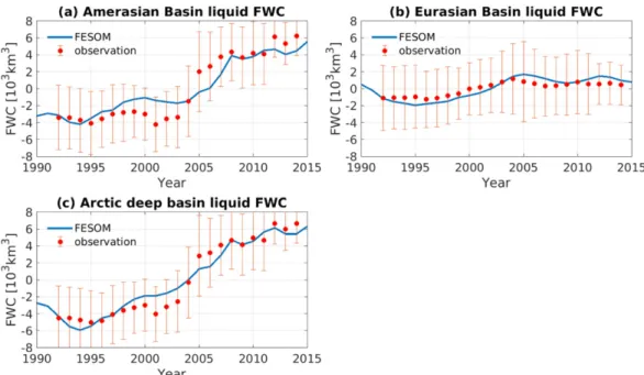
Observations have revealed a positive trend in the Arctic liquid FWC starting from the mid-1990s (Proshutinsky et al. 2009; McPhee et al. 2009; Rabe et al. 2011; Giles et al. 2012; Polyakov et al. 2013).
Figure 3shows the liquid FWC2in the two Arctic deep ocean basins and their sum obtained from the control simulation. The two deep basins are the Arctic areas with ocean bathymetry deeper than 500 m, separated by the Lomonosov Ridge (Fig. 1, upper panel). The simu- lated Arctic liquid FWC well represents the observed trend. The upward trend of the Arctic liquid FWC was profound before 2010 and became weaker afterward. It is clear fromFig. 3that the trend of the Arctic liquid
FWC mainly stems from that in the Amerasian basin. In the Eurasian basin the liquid FWC increased slowly before 2005. When the FWC in the Amerasian basin increases rapidly between 2005 and 2009, the FWC in the Eurasian basin decreases slightly, which is consistent with observations reported before (McPhee et al. 2009;
Morison et al. 2012).
Previous studies have suggested that wind-driven con- vergence drives the accumulation of freshwater in the Beaufort Gyre and Amerasian basin (e.g., Proshutinsky et al. 2002,2015;Koldunov et al. 2014). Indeed, the sim- ulated rapid increase of liquid FWC in the Amerasian basin during the second half of the 2000s in the control is accompanied by a large positive anomaly in the sea level pressure over the Beaufort Gyre region, an indication of the anticyclonic regime of the atmospheric circulation (cf.Figs. 4a,c). At the beginning of the 2010s, the wind regime became neutral to cyclonic (Fig. 4b), so the rapid increase of FWC in the Canada basin stopped, although there is some freshwater accumulated in the Makarov basin (Fig. 4d).
Significant sea ice loss has been observed in the recent decades (Kwok et al. 2009;Stroeve et al. 2012;Laxon et al. 2013). The control simulation reproduces the ob- served declining trend of sea ice in the period 2001–15 reasonably well, as shown by the plots of anomalies in Fig. S1 in the online supplemental material. In the sen- sitivity experiment, the air temperature and downward radiation fluxes in the Arctic region are kept at their
FIG. 3. Anomaly of liquid FWC in the (a) Amerasian basin, (b) Eurasian basin, and (c) Arctic deep basin (sum of the two basins). The liquid FWC observation is described inRabe et al. (2014). See footnote 2 for the definition of the FWC.
2FWC is calculated as Ð Ð Ð0
D(Sref2S)/Srefdxdydz, whereSis salinity,Sref534:8 is the reference salinity, and Dis the depth where salinity is equal to the reference salinity. We will also discuss the spatial pattern of FWC, the vertically integrated freshwater amountÐ0
D(Sref2S)/Srefdz. In the calculation of FWC from ob- servations (shown inFig. 3),Rabe et al. (2014)took a different definition. They used the reference salinity of 35 and integrated from the ocean surface to the 34 isohaline depth. The different definition can lead to a difference in the mean value of the FWC, while the anomalies of the FWC time series remain nearly the same (not shown).
1 JANUARY2019 W A N G E T A L . 19
FIG. 4. Sea level pressure (SLP) anomaly referenced to 1971–2015 for the periods (a) 2005–09 and (b) 2010–15.
(c) The difference of liquid freshwater content (m) between 2009 and 2004 in the control run. (d) As in (c), but for the difference between 2015 and 2009. (e),(f) As in (c) and (d), but for the climatology run. The black contour lines in (c)–(f) indicate the 500-, 2000-, and 3500-m isobaths.
climatological values, so the sea ice concentration and thickness are larger than in the control run (Figs. S2a,b), with the rapid Arctic sea ice decline eliminated (Fig. 2b).
Some variability in the Arctic sea ice volume and net thermodynamic growth rate is retained (Figs. 2b,c), owing to variations in factors such as near surface atmospheric winds.
In the following we will present the result of the sen- sitivity experiment (the climatology run) and compare it to the control run. As the control run is the hindcast simulation representing the realistic case with atmo- spheric warming and the atmospheric warming in the thermal forcing is removed in the climatology run, the difference in the simulated liquid freshwater between the two runs can be attributed to the atmospheric warm- ing. Insection 4cwe will prove that the induced sea ice decline by the atmospheric warming is the main direct cause for the difference between the two runs.
Under the anticyclonic wind regime from 2005 to 2009, the FWC in the Amerasian basin also increases in the climatology run (Fig. 4e). However, the magnitude of the increase is much smaller than in the control run (cf.Figs. 4c,e). In addition, the relatively strong decrease of FWC in the eastern Eurasian basin in the control is not present in the climatology run. From 2009 to 2015, the FWC in the Beaufort Gyre region decreases in the climatology run (Fig. 4f). Both simulations indicate that the atmospheric circulation regime determines the phase of the Arctic freshwater accumulation and re- lease. However, the changes in the spatial pattern of
FWC are so different between the two simulations, im- plying significant impacts of the sea ice loss.
The time series of the FWC integrated over the Arctic Ocean and over different Arctic basins can better illustrate the quantitative impact of the sea ice loss (Fig. 5). In the Amerasian basin, the FWC increases before 2009 in both simulations, while the rise in the climatology run is signif- icantly smaller (Fig. 5a). Afterward, the Amerasian basin FWC stays at the high level and continues to increase with a low rate in the control run. On the contrary, it has a decreasing tendency in the climatology run.
In the Eurasian basin, the FWC in the control has a small decreasing tendency after 2005, whereas it shows an increasing trend in the climatology run (Fig. 5b). As a result, the sum of the FWC in the two deep basins is very similar between the two simulations (Fig. 5c). The total liquid FWC of the Arctic Ocean including the conti- nental shelves has an even smaller difference (Fig. 5d).
b. Constituents of the FWC changes
Intuitively one might expect that ocean surface freshening caused by the sea ice loss (the net melting) would have contributed to the increase of the Arctic liquid FWC in the past decades. Our simulations show that the Arctic liquid FWCs in the two simulations are surprisingly similar (Figs. 5c,d), although sea ice loss does significantly modify the spatial distribution of the freshwater (Fig. 4). What is the reason for this intriguing behavior? In the following we will look into water mass components and try to understand the reason.
FIG. 5. Anomaly of the liquid FWC in the (a) Amerasian basin, (b) Eurasian basin, (c) Arctic deep basin (sum of the two basins), and (d) the whole Arctic Ocean in the two simulations.
1 JANUARY2019 W A N G E T A L . 21
The sea ice decline leads to changes in all the com- ponents of the freshwater budget (Fig. 6).3In the Am- erasian basin, the change in the sea ice thermodynamic growth rate has the largest contribution to the difference of the FWC between the runs, as shown by the fresh- water passive tracers inFig. 6a. The contributions from other surface freshwater fluxes are smaller. The values of dye tracers represent the proportion of the associated water masses. The proportions of water masses origi- nating from the Bering Strait and Barents Sea Opening in the Amerasian basin are enlarged by the sea ice de- cline as revealed by the dye tracers (positive values;
Fig. 6c).
Although the increment of FWC due to the change of the sea ice thermodynamic growth rate can largely ex- plain the enhanced freshwater storage in the Amerasian basin (Fig. 6a), it does not explain all the difference in the FWC spatial pattern between the two runs (cf.
Figs. 7a,b). The difference in the FWC has higher values
in the gyre center, because the sea ice decline also causes other freshwater masses to accumulate toward the cen- ter of the Amerasian basin, including river water, snow meltwater and Pacific Water (Fig. 7).
In the Eurasian basin, different surface water fluxes tend to increase the FWC in the case of sea ice decline, except for the slightly enhanced evaporation (Fig. 6b).
Despite the overall freshening effect from surface sources, the FWC in the Eurasian basin is lower in the control run (Fig. 6b), which can only be explained by the increase in the proportion of saline AW and the de- crease in the proportion of fresh Pacific Water (Fig. 6d).
Among the total AW contribution, the Barents Sea branch AW accounts for more than 80% of the increase in the AW proportion in the case of sea ice decline.
The model results presented above clearly show that the sea ice decline can influence the Arctic liquid FWC through both freshening the upper ocean (reduction of the net sea ice thermodynamic growth rate) and modi- fying the spatial distribution of different water masses (Figs. 6and7). It causes the water masses in the upper ocean to shift from the Siberian Shelf and Eurasian basin side toward the Amerasian basin. On the one hand, the liquid FWC in the Amerasian basin is increased by the sea ice decline, mainly through the supply of sea ice meltwater. On the other hand, the FWC in the Eurasian basin is reduced, mainly through the replacement of fresh Pacific Water by saline AW in the upper ocean.
FIG. 6. (a) The difference of liquid FWC between the two simulations (control minus climatology) in the Am- erasian basin, and the individual contributions from sea ice thermodynamic growth rate, evaporation, precipitation, and river water. (b) As in (a), but for the Eurasian basin. (c) The difference of the Arctic inflow passive tracers averaged above theS534.8 isohaline in the Amerasian basin between the two simulations. (d) As in (c), but for the Eurasian basin.
3To illustrate the difference between the two simulations, we plot ‘‘control run minus sensitivity run’’ inFigs. 6–10, rather than
‘‘sensitivity minus control’’ as usually taken. This is because the control run represents the Arctic warming and sea ice loss scenario, while the sensitivity run represents a climatological state. Logically it makes sense to discuss the impact of sea ice decline compared to the climatological state, so it is preferable to show control minus sensitivity.
Overall, the Arctic total liquid FWC is not significantly changed by the sea ice decline in the period of 2001–15.
4. Discussion
a. Impact of sea ice decline
The variability of the upper Arctic Ocean circulation and freshwater accumulation is predominantly driven by the variation of the wind forcing (Proshutinsky et al.
2002, 2015; Zhang et al. 2003; Condron et al. 2009;
Rudels 2012). It is known that the atmospheric circula- tion regime not only influences the location of the front between upper waters derived from the Atlantic and Pacific Oceans (Carmack et al. 1995;McLaughlin et al.
1996;Morison et al. 1998,2006;Alkire et al. 2007), but also impacts the pathway of the low-salinity shelf water originating from the Siberian Shelf (Proshutinsky and Johnson 1997;Steele and Boyd 1998; Polyakov et al.
1999; Maslowski et al. 2000; Anderson et al. 2004;
Newton et al. 2008; Timmermans et al. 2011). The
FIG. 7. (a) Difference of freshwater content (m) between the control and climatology runs, and differences of freshwater content associated with different sources between the two simulations: (b) sea ice thermodynamic growth rate, (c) river water, (d) evaporation, and (e) precipitation. (f) Difference of the Barents Sea Opening (BSO) passive tracer vertically averaged above theS534.8 isohaline between the two runs. (g),(h) As in (f), but for the Fram Strait (FS) and Bering Strait (BS) passive tracers, respectively. The mean fields averaged over 2011–15 are shown. The black contour lines indicate the 500-, 2000-, and 3500-m isobaths.
1 JANUARY2019 W A N G E T A L . 23
propagation of water masses over the Siberian Shelf, either along the continental shelf or into the deep ocean basin, was found to be very sensitive to the wind forcing (Steele and Ermold 2004;Dmitrenko et al. 2008;Bauch et al. 2009). Changes in the atmospheric circulation re- gimes can also modulate the pathway of river water and alter its distribution between the Arctic deep basins (Morison et al. 2012). The aforementioned studies have revealed the importance of wind forcing in driving the Arctic upper ocean circulation and liquid FWC vari- ability. This work further emphasizes that sea ice me- diates the wind-driven ocean circulation, which should be considered when it comes to assessing the causes of the change in the Arctic liquid FWC.
When sea ice declines, resulting in lower thickness and concentration, it moves faster (Rampal et al. 2009;
Zhang et al. 2012;Kwok et al. 2013) and shows an am- plified anticyclonic circulation around the Beaufort Gyre (Petty et al. 2016). As expected, the sea ice circulation in the Beaufort Gyre (anticyclonic) and along the Trans- polar Drift (toward the Fram Strait) is stronger in our control run (Figs. 8a,b). The reduction in sea ice cover and the speeding up of sea ice drift can modify the ocean surface stress (Martin et al. 2014). In our simu- lations the ocean surface stress is significantly modified by the sea ice loss (Fig. 8c), producing a difference in the surface Ekman transport (Fig. 8d). The offshore transport from the Siberian Shelf to the Eurasian basin and the convergence in the Beaufort Sea region is enhanced.
The difference in the upper ocean velocity between the two simulations shows an anticlockwise circulation anomaly in the Eurasian basin and a clockwise anomaly in the Amerasian basin (Fig. 8e). This difference re- sembles the difference of the ocean surface geostrophic velocity between the two runs (Fig. 8f), which is asso- ciated with the difference in the sea surface height (Fig. S3). The latter is due to the change in the steric height, hence mainly due to the FWC change (e.g., Armitage et al. 2016). That is, the difference in the surface geostrophic velocity corresponds to the increase of FWC in the Amerasian basin and the decrease in the Eurasian basin caused by the sea ice decline (Fig. 7a).
As shown inFigs. 6b and 6d, the reduction in the FWC in the Eurasian basin is mainly caused by the decrease of the Pacific Water and increase of the AW proportions.
The enhanced offshore Ekman transport carries the shelf water consisting of Barents Sea branch AW and river runoff water to the Eurasian basin, which increases the AW proportion in the ocean freshwater layer of the Eurasian basin. When the Ekman transport anomaly shifts surface waters from the Eurasian basin toward the Lomonosov Ridge, the strengthened anticyclonic ocean
circulation in the Amerasian basin can also confine the Pacific Water to the western side of the Lomonosov Ridge, further reducing the Pacific Water proportion in the Eurasian basin. That is, sea ice meltwater and changes in ocean surface stress can lead to changes in upper ocean circulation, thus modifying the freshwa- ter spatial distribution, while the modified freshwa- ter spatial distribution may further influence the surface geostrophic current, thus the upper ocean circulation.
Therefore, the impact of sea ice decline on the spatial distribution of water masses and the liquid FWC very possibly invokes interactive dynamical processes. By us- ing the online passive tracers, we revealed the details of the overall consequences of the sea ice decline in this study.
Within the studied period, the most rapid change in the local FWC and water mass proportion (Pacific and Atlantic Waters) in the Eurasian basin related to sea ice decline took place in the second half of the 2000s (Figs. 6b,d), which is in phase with a strong anticyclonic atmospheric circulation (Fig. 4a). We speculate that the sea ice decline would have produced an opposite dy- namical effect on the ocean circulation and regional FWC if a cyclonic atmospheric circulation had domi- nated. The atmospheric circulation over the Arctic Ocean is predominantly cyclonic in 2012 (Fig. S4). In- deed, there is a local minimum in the anomaly of the AW proportion and a local maximum in the anomaly of the Pacific Water proportion in the Eurasian basin in this particular year, as shown by the time series in Fig. 6d. However, we do not expect that the sea ice de- cline just acts as a simple multiplier to the effect of winds on the ocean circulation, because it is not spatially uni- form, with the periphery of the Arctic Ocean being more vulnerable to the warming climate (Fig. S2a).
By using a coupled climate modelLique et al. (2018) showed that the Amerasian basin will become fresher while the Eurasian basin will become more saline due to sea ice decline in future warmer climate (in a 43CO2 scenario). Our study indicates that the sea ice decline in the past decade has already started this changing ten- dency. However, as discussed above, the atmospheric circulation regime also plays a key role. We suggest that the recently observed winter ventilation in the eastern Eurasian basin (Polyakov et al. 2017) is at least partly due to the reduction of stratification associated with salinification of the upper ocean caused by sea ice de- cline as revealed in our study.
The sea ice decline is identified as an important fac- tor that can modify the fate of the Barents Sea branch AW after it enters the Siberian Shelf. We find that the Barents Sea branch AW inflow is not significantly changed between the two simulations, so the increased
FIG. 8. (a) Difference of sea ice drift velocity between the control run and the climatology run in winter (February–April). (b) As in (a), but for summer (August–October). Difference of (c) ocean surface stress, (d) Ekman transport, (e) upper 200-m ocean velocity, and (f) ocean surface geostrophic velocity between the two runs. The average over the last 10 years is shown. The vectors represent the mean fields averaged over 200 km3200 km boxes. The gray contour lines indicate the 500-, 2000-, and 3500-m isobaths.
1 JANUARY2019 W A N G E T A L . 25
AW proportion in the freshwater layer means a reduced AW supply to the denser ocean layers below. Indeed this is found in the model results (Fig. S5). The stronger offshore Ekman transport enhances the export of the upper ocean water masses into the basin in the case of sea ice decline (Fig. 8d). The increased export of water masses of AW origin in the upper ocean layer can reduce the amount of AW in formed dense water, thus its supply to the deep ocean layers of the Arctic basin. The importance of ocean surface stress in controlling shelf- to-basin transport of shelf water masses is consistent with findings in previous studies focused on the Siberian Shelf (Steele and Ermold 2004;Dmitrenko et al. 2008;
Bauch et al. 2009) and other Arctic shelf regions (Watanabe 2013). Our study further reveals that the impact of ocean surface stress and sea ice decline on the supply of water masses of AW origin to the Arctic basin reaches both the upper and deep ocean.
Meanwhile the anticlockwise ocean velocity anomaly in the Eurasian basin (Fig. 8f) also enhances the AW inflow from the Fram Strait, accounting for less than 20% of the total increase in the AW proportion in the freshwater layer. Although its contribution to the changes of the liquid FWC is relatively small compared to the larger changes of the Barents Sea branch AW and the Pacific Water, the Fram Strait inflow can also impact the deep AW layer circulation. Previous studies have indicated that weaker sea ice and changes in ocean surface circulation can influence the AW layer circula- tion located at depth (Karcher et al. 2012;Itkin et al.
2014;Lique et al. 2015). In this paper we focus on the Arctic surface freshwater, while the model results in- dicate that dedicated future work is needed to better understand the processes that can influence the fate of the AW in the Arctic Ocean in a changing climate, in particular, in terms of possible changes in the AW layer circulation. For example, Arctic warming can change the surface properties in the Barents Sea, and thus the Barents Sea Water formed there; this signal can propa- gate to the Arctic basin within the AW layer. Recent climate model simulations imply that AW circulation at Fram Strait and in the Eurasian basin might also change in a warming climate (Lique et al. 2018).
b. Other implications of the Arctic sea ice decline By analyzing available observational data Peralta- Ferriz and Woodgate (2015)found that the interannual variability and trend of the Arctic basin mixed layer depth (MLD) is mainly determined by the changes in the upper ocean salinity. They showed that the MLD in the Arctic basins has a large seasonal variation. Aver- aged over last three decades, the observed Arctic MLD in summer is about 10–20 m. In winter, it is about 30 and
70 m in the Canada and Eurasian basins, respectively.
The control run reproduced the seasonal and spatial variation in the MLD (Figs. 9a,c). The winter MLD in the Canada basin in the period 2011–15 is deeper than the observational long-term mean. However, the simu- lated winter MLD averaged over the last three decades compares well with the observational estimate (Fig. S6).
This implies that the decadal variability of winter MLD in the Canada basin is significant, and it is in a deeper state in the first half of 2010s.
Sea ice decline changes not only the freshwater spatial distribution, but also the MLD (Figs. 9b,d). It has a larger impact on the MLD in winter than in summer. In the Amerasian basin it causes significant surface fresh- ening, which in turn stabilizes the upper ocean and re- duces the winter MLD by 20–40 m. The winter MLD in the Eurasian basin is less significantly changed (about 10 m), as the change of the upper ocean salinity and stratification is smaller than in the Amerasian basin.
Larger MLD in part of the Barents Sea and near the Fram Strait is simulated in the case with sea ice decline.
The larger MLD is presumably associated with the local increase of sea ice production, and thus brine rejection, in those regions (cf. Fig. S2c). The revealed impact of the sea ice decline on the Arctic basin MLD has a strong implication on biogeochemical processes, as winter MLD is one of the key factors regulating summer primary production (e.g.,Popova et al. 2010).
Sea ice decline affects not only the ocean circulation inside the Arctic Ocean, but also the freshwater outflow to the North Atlantic. The liquid freshwater export through the Davis Strait is increased, while it is reduced at Fram Strait (Fig. 10), which is consistent with the redistribution of freshwater between the two Arctic basins (fresher north of the Canadian Arctic Archi- pelago and more saline north of Fram Strait). The sea ice solid freshwater export decreases with sea ice thinning (Fig. 10), even though the sea ice drift be- comes faster at the same time (Figs. 8a,b). The changes in the liquid freshwater export through the two straits do not fully compensate, but the change in the total liquid freshwater export has a smaller magnitude than that of the solid freshwater. Thus the total freshwater export to the North Atlantic is reduced by the sea ice decline, mainly due to the reduction in the solid fresh- water export.
c. Attributing the change of freshwater spatial distribution
The only difference in the model configurations be- tween the two simulations is the thermal forcing over the Arctic Ocean (in terms of air temperature and down- ward radiation), to which the change in the upper ocean
circulation and liquid FWC described above should be attributed. Besides causing sea ice decline, the warmer atmosphere also increases the ocean temperature over the continental shelves, most significantly in the Barents and Kara Seas (up to 28C at the surface and 18C at 100-m depth), as indicated by the difference in the temperature between the two simulations (Fig. S7). In these shelf regions sea ice cover retreats more strongly (Fig. S2a).
The temperature increase in the halocline of the deep ocean basins is relatively small (less than 0.18C).
The change in ocean temperature may impact ocean density, and thus ocean circulation. Did the profound ocean warming over the continental shelves significantly contribute to changes in the upper ocean circulation and thus water mass spatial distribution? Or, should we at- tribute the change in FWC spatial distribution between the two runs mainly to sea ice decline, or to both the sea ice decline and ocean warming? To answer these
questions we carried out an additional experiment. It is the same as the climatology run except that we modified the calculation of ocean density during the simulation.
We computed the monthly temperature difference be- tween the results from the control and climatology runs, and then added it to the ocean temperature in the calculation of the ocean density over the continental shelves during the new model run. Note that the tem- perature difference is not added to the prognostic tem- perature field of the model, otherwise the sea ice state would be changed due to the additional ocean heat. We found that the liquid FWC is not significantly changed when the ocean density change induced by the ocean warming is incorporated (Fig. S8). As the ocean warm- ing does not have a significant impact, the change in the FWC spatial distribution between the control and cli- matology runs should be mainly attributed to the direct effect of sea ice decline.
FIG. 9. (a) The winter (March and April) mixed layer depth (MLD) averaged in the period 2011–15 in the control run and (b) the difference from the climatology run. (c),(d) As in (a) and (b) but for summer (July and August).
Note that different color ranges are used in the plots. The black contour lines indicate the 500-, 2000-, and 3500-m isobaths.
1 JANUARY2019 W A N G E T A L . 27
d. Short comments on the interpretation of model results
1) ABOUT USING FORCED OCEAN MODEL SIMULATIONS
In this study we tried to elucidate the impact of the sea ice decline on the Arctic liquid freshwater storage for the period 2001–15, when both the Arctic sea ice and liquid freshwater have reached a new climate state. We used forced model simulations to distinguish the effect of sea ice decline from effects related to other forcing fields. In the sensitivity experiment we changed the air temperature and downward radiation to the climato- logical state, but kept the wind field the same as in the hindcast simulation. In the climate system or a coupled climate model, changes in the atmospheric thermal forcing and sea ice state will certainly change wind fields.
However, our interest in this work is to understand the role of sea ice decline in one particular climate trajec- tory, the historical one. We want to know how much of the observed changes in the Arctic freshwater can be attributed to the direct role of sea ice decline, which motivated our usage of a forced ice–ocean model and the experimental design.
2) ABOUT SIMULATION BIASES IN THE MODEL
As shown in previous model intercomparison studies, state-of-the-art ocean–sea ice models have very large model spread in their simulated Arctic sea ice and freshwater, especially for the mean state (e.g.,Jahn et al.
2012;Aksenov et al. 2016;Wang et al. 2016b,c). In our case, the simulated mean FWC is higher than observa- tions and the anticyclonic ocean circulation spans a too large area (Fig. S9). Accordingly, the location of the
Transpolar Drift and the front between the Pacific and Atlantic Waters is biased toward the Siberian Shelf.
Therefore, the quantitative results about the proportion of different surface water masses located in the two geometrically defined basins (Amerasian and Eurasian Basins) are mainly intended to help understand the role of sea ice decline in spatially shifting water masses.
Previous studies also show that using more elaborated parameterizations of ice drag by taking into account evolving sea ice properties can influence simulated sea ice state (Tsamados et al. 2014;Martin et al. 2016), thus possibly modifying upper ocean circulation. Employing these parameterizations may therefore impact the quan- titative model results. The fact that the control simu- lation well reproduces the observed variation of the liquid FWC and sea ice state in the studied period gives us the credence that the revealed response of the upper ocean circulation and liquid FWC to sea ice decline is plausible.
5. Conclusions
In this study we used global ocean–sea ice model simulations to understand the impact of sea ice decline on the Arctic liquid FWC for the period 2001–15. This is a very special period under the ongoing climate change: The Arctic summer sea ice extent reached its record low, while the Arctic liquid freshwater storage reached its record high. We carried out a sensitivity experiment that is forced by climatological air temper- ature and downward radiation fluxes in the Arctic region to eliminate the sea ice decline. By comparing this simulation with a hindcast simulation that adequately represents the decline of the sea ice and the variability of liquid FWC in the Arctic Ocean, we investigated the in- fluence of the recent sea ice decline on the evolution of the Arctic liquid FWC and the freshwater spatial distribution.
The sea ice decline contributes to changes in the Arctic liquid FWC in two ways. First, the sea ice melting (reduction in the net sea ice thermodynamic growth rate) reduces the upper ocean salinity, thus tending to increase the Arctic liquid FWC. This effect is more pronounced in the Amerasian basin. Second, the sea ice decline alters the ocean surface stress and upper ocean circulation, thus changing the spatial distribution of different water masses. This effect turns out to be of vital importance. It helps to export upper ocean water masses from the Siberian Shelf toward the deep ocean basin.
Therefore, the proportion of saline AW in the upper ocean of the Eurasian basin is increased, along with the retreat of the fresh Pacific Water to the Amerasian ba- sin. The increase of the liquid FWC in the Amerasian basin is nearly compensated by the reduction in the
FIG. 10. Difference of freshwater export fluxes (mSv; 1 Sv[ 106m3s21) between the control and climatology runs. A positive value means larger export.
Eurasian basin, so the total Arctic liquid FWC is not significantly changed by the sea ice decline.
Although the sea ice decline does not change the total Arctic liquid FWC, it results in significant changes in the spatial distribution of the liquid FWC. In particular, about half of the liquid FWC accumulated in the Amer- asian basin during the 15-yr period simulated in the model can be attributed to the sea ice decline (6.613103km3 freshwater accumulated in the case of sea ice decline versus 3.473103km3without sea ice decline). Our work suggests that the two impact pathways of sea ice decline, directly freshening the ocean and changing the ocean cir- culation, should be considered simultaneously in order to adequately understand and predict the evolution of the Arctic freshwater condition under a changing climate.
The winter MLD in the Amerasian basin is significantly reduced by the upper ocean freshening induced by the sea ice decline, implying that both the physical and bio- geochemical environments of the Arctic Ocean have been modified by the sea ice decline. The total freshwater ex- port to the North Atlantic is reduced by the sea ice decline, mainly owing to the decrease of the sea ice volume export.
The impact of the recent Arctic sea ice decline on the Atlantic meridional overturning circulation on decadal time scales remains to be explored in future work.
We suggest that the response of dynamical processes over the Siberian Shelf and along the Arctic continental slope to the ongoing sea ice decline merits further dedi- cated studies. Sustaining long-term observational systems in these regions will be very useful for monitoring and understanding the local ocean changes that are relevant for the large-scale Arctic Ocean circulation and environment.
Acknowledgments. This work was supported by the Helmholtz Climate Initiative REKLIM (Regional Climate Change), the AWI FRAM (Frontiers in Arctic Marine Monitoring) program, the project of the Col- laborative Research Centre TRR 181 ‘‘Energy Trans- fer in Atmosphere and Ocean’’ (S1 and S2) funded by the German Research Foundation, the EC project PRIMAVERA under grant agreement 641727, and the state assignment of FASO Russia (theme 0149-2018- 0014). We thank Patrick Scholz for helping us to create the grid resolution plot of Fig. 1 and the anonymous reviewers and the editor for very helpful comments.
The simulations were performed at the North-German Supercomputing Alliance (HLRN).
REFERENCES
Aagaard, K., J. H. Swift, and E. Carmack, 1985: Thermohaline circulation in the Arctic Mediterranean seas.J. Geophys. Res., 90, 4833–4846,https://doi.org/10.1029/JC090iC03p04833.
Aksenov, Y., and Coauthors, 2016: Arctic pathways of Pacific Water: Arctic Ocean model intercomparison experiments.
J. Geophys. Res. Oceans,121, 27–59,https://doi.org/10.1002/
2015JC011299.
Alkire, M. B., K. Falkner, I. Rigor, M. Steele, and J. Morison, 2007:
The return of Pacific waters to the upper layers of the central Arctic Ocean.Deep-Sea Res. I,54, 1509–1529,https://doi.org/
10.1016/j.dsr.2007.06.004.
——, J. Morison, A. Schweiger, J. Zhang, M. Steele, C. Peralta- Ferriz, and S. Dickinson, 2017: A meteoric water budget for the Arctic Ocean.J. Geophys. Res. Oceans,122, 10 020–10 041, https://doi.org/10.1002/2017JC012807.
Anderson, L., S. Jutterström, S. Kaltin, E. Jones, and G. Björk, 2004: Variability in river runoff distribution in the Eurasian basin of the Arctic Ocean.J. Geophys. Res.,109, C01016, https://doi.org/10.1029/2003JC001773.
Armitage, T., S. Bacon, A. Ridout, S. Thomas, Y. Aksenov, and D. Wingham, 2016: Arctic sea surface height variability and change from satellite radar altimetry and GRACE, 2003–2014.
J. Geophys. Res. Oceans, 121, 4303–4322, https://doi.org/
10.1002/2015JC011579.
Arzel, O., T. Fichefet, H. Goosse, and J.-L. Dufresne, 2008: Causes and impacts of changes in the Arctic freshwater budget during the twentieth and twenty-first centuries in an AOGCM.Climate Dyn.,30, 37–58,https://doi.org/10.1007/
s00382-007-0258-5.
Bauch, D., I. Dmitrenko, C. Wegner, J. Holemann, S. Kirillov, L. Timokhov, and H. Kassens, 2009: Exchange of Laptev Sea and Arctic Ocean halocline waters in response to atmospheric forcing.J. Geophys. Res.,114, C05008,https://doi.org/10.1029/
2008JC005062.
Carmack, E. C., R. Macdonald, R. G. Perkin, F. A. McLaughlin, and R. J. Pearson, 1995: Evidence for warming of Atlantic water in the southern Canadian Basin of the Arctic Ocean:
Results from the Larsen-93 Expedition.Geophys. Res. Lett., 22, 1061–1064,https://doi.org/10.1029/95GL00808.
——, and Coauthors, 2016: Freshwater and its role in the Arctic Marine System: Sources, disposition, storage, export, and physical and biogeochemical consequences in the Arctic and global oceans.J. Geophys. Res. Biogeosci.,121, 675–717, https://doi.org/10.1002/2015JG003140.
Condron, A., P. Winsor, C. Hill, and D. Menemenlis, 2009: Simu- lated response of the Arctic freshwater budget to extreme NAO wind forcing.J. Climate,22, 2422–2437,https://doi.org/
10.1175/2008JCLI2626.1.
Danabasoglu, G., and Coauthors, 2014: North Atlantic simulations in Coordinated Ocean-ice Reference Experiments phase II (CORE-II). Part I: Mean states.Ocean Modell.,73, 76–107, https://doi.org/10.1016/j.ocemod.2013.10.005.
Danilov, S., Q. Wang, R. Timmermann, N. Iakovlev, D. Sidorenko, M. Kimmritz, T. Jung, and J. Schröter, 2015: Finite-Element Sea Ice Model (FESIM), version 2.Geosci. Model Dev.,8, 1747–1761,https://doi.org/10.5194/gmd-8-1747-2015.
Dickson, R., B. Rudels, S. Dye, M. Karcher, J. Meincke, and I. Yashayaev, 2007: Current estimates of freshwater flux through Arctic and subarctic seas.Prog. Oceanogr.,73, 210–
230,https://doi.org/10.1016/j.pocean.2006.12.003.
Dmitrenko, I. A., S. Kirillov, and L. Tremblay, 2008: The long-term and interannual variability of summer fresh water storage over the eastern Siberian Shelf: Implication for climatic change.J. Geophys.
Res.,113, C03007,https://doi.org/10.1029/2007JC004304.
——, V. V. Ivanov, S. A. Kirillov, E. L. Vinogradova, S. Torres- Valdes, and D. Bauch, 2011: Properties of the Atlantic derived
1 JANUARY2019 W A N G E T A L . 29
halocline waters over the Laptev Sea continental margin:
Evidence from 2002 to 2009.J. Geophys. Res.,116, C10024, https://doi.org/10.1029/2011JC007269.
Giles, K. A., S. W. Laxon, A. L. Ridout, D. J. Wingham, and S. Bacon, 2012: Western Arctic Ocean freshwater storage increased by wind-driven spin-up of the Beaufort Gyre.Nat.
Geosci.,5, 194–197,https://doi.org/10.1038/ngeo1379.
Haine, T., and Coauthors, 2015: Arctic freshwater export: Status, mechanisms, and prospects.Global Planet. Change,125, 13–
35,https://doi.org/10.1016/j.gloplacha.2014.11.013.
Itkin, P., M. Karcher, and R. Gerdes, 2014: Is weaker Arctic sea ice changing the Atlantic water circulation?J. Geophys. Res. Oceans, 119, 5992–6009,https://doi.org/10.1002/2013JC009633.
Jahn, A., and Coauthors, 2012: Arctic Ocean freshwater: How ro- bust are model simulations?J. Geophys. Res.,117, C00D16, https://doi.org/10.1029/2012JC007907.
Jakobsson, M., R. Macnab, L. Mayer, R. Anderson, M. Edwards, J. Hatzky, H. W. Schenke, and P. Johnson, 2008: An improved bathymetric portrayal of the Arctic Ocean: Implications for ocean modeling and geological, geophysical and oceano- graphic analyses. Geophys. Res. Lett., 35, L07602, https://
doi.org/10.1029/2008GL033520.
Johnson, H. L., S. B. Cornish, Y. Kostov, E. Beer, and C. Lique, 2018: Arctic Ocean freshwater content and its decadal mem- ory of sea-level pressure.Geophys. Res. Lett.,45, 4991–5001, https://doi.org/10.1029/2017GL076870.
Karcher, M., J. Smith, F. Kauker, R. Gerdes, and W. Smethie, 2012:
Recent changes in Arctic Ocean circulation revealed by iodine-129 observations and modeling.J. Geophys. Res.,117, C08007,https://doi.org/10.1029/2011JC007513.
Kobayashi, S., and Coauthors, 2015: The JRA-55 reanalysis:
General specifications and basic characteristics. J. Meteor.
Soc. Japan,93, 5–48,https://doi.org/10.2151/jmsj.2015-001.
Koldunov, N. V., and Coauthors, 2014: Multimodel simulations of Arctic Ocean sea surface height variability in the period 1970–
2009.J. Geophys. Res. Oceans,119, 8936–8954,https://doi.org/
10.1002/2014JC010170.
Krishfield, R. A., A. Proshutinsky, K. Tateyama, W. J. Williams, E. C.
Carmack, M. F. A., and M. L. Timmermans, 2014: Deterioration of perennial sea ice in the Beaufort Gyre from 2003 to 2012 and its impact on the oceanic freshwater cycle.J. Geophys. Res. Oceans, 119, 1271–1305,https://doi.org/10.1002/2013JC008999.
Kwok, R., G. F. Cunningham, M. Wensnahan, I. Rigor, H. J.
Zwally, and D. Yi, 2009: Thinning and volume loss of the Arctic Ocean sea ice cover: 2003–2008.J. Geophys. Res.,114, C07005,https://doi.org/10.1029/2009JC005312.
——, G. Spreen, and S. Pang, 2013: Arctic sea ice circulation and drift speed: Decadal trends and ocean currents. J. Geophys. Res.
Oceans,118, 2408–2425,https://doi.org/10.1002/jgrc.20191.
Large, W. G., and S. G. Yeager, 2009: The global climatology of an interannually varying air–sea flux data set.Climate Dyn.,33, 341–364,https://doi.org/10.1007/s00382-008-0441-3.
——, J. C. McWilliams, and S. C. Doney, 1994: Oceanic vertical mixing—A review and a model with a nonlocal boundary- layer parameterization. Rev. Geophys.,32, 363–403,https://
doi.org/10.1029/94RG01872.
Laxon, S. W., and Coauthors, 2013: CryoSat-2 estimates of Arctic sea ice thickness and volume.Geophys. Res. Lett.,40, 732–737, https://doi.org/10.1002/grl.50193.
Lique, C., H. L. Johnson, and P. E. D. Davis, 2015: On the interplay between the circulation in the surface and the intermediate layers of the Arctic Ocean.J. Phys. Oceanogr.,45, 1393–1409, https://doi.org/10.1175/JPO-D-14-0183.1.
——, ——, and Y. Plancherel, 2018: Emergence of deep convection in the Arctic Ocean under a warming climate.Climate Dyn., 50, 3833–3847,https://doi.org/10.1007/s00382-017-3849-9.
Martin, T., M. Steele, and J. Zhang, 2014: Seasonality and long- term trend of Arctic Ocean surface stress in a model.J. Geo- phys. Res. Oceans, 119, 1723–1738, https://doi.org/10.1002/
2013JC009425.
——, M. Tsamados, D. Schroeder, and D. L. Feltham, 2016: The impact of variable sea ice roughness on changes in Arctic Ocean surface stress: A model study.J. Geophys. Res. Oceans, 121, 1931–1952,https://doi.org/10.1002/2015JC011186.
Maslowski, W., B. Newton, P. Schlosser, A. Semtner, and D. Martinson, 2000: Modeling recent climate variability in the Arctic Ocean.
Geophys. Res. Lett., 27, 3743–3746, https://doi.org/10.1029/
1999GL011227.
McLaughlin, F., E. Carmack, R. Macdonald, and J. Bishop, 1996:
Physical and geochemical properties across the Atlantic/
Pacific water mass front in the southern Canadian Basin.
J. Geophys. Res., 101, 1183–1197, https://doi.org/10.1029/
95JC02634.
McPhee, M. G., T. P. Stanton, J. H. Morison, and D. G. Martinson, 1998: Freshening of the upper ocean in the Arctic: Is perennial sea ice disappearing? Geophys. Res. Lett., 25, 1729–1732, https://doi.org/10.1029/98GL00933.
——, A. Proshutinsky, J. H. Morison, M. Steele, and M. B. Alkire, 2009: Rapid change in freshwater content of the Arctic Ocean.
Geophys. Res. Lett., 36, L10602, https://doi.org/10.1029/
2009GL037525.
Morison, J., M. Steele, and R. Andersen, 1998: Hydrography of the upper Arctic Ocean measured from the nuclear submarine U.S.S. Pargo.Deep-Sea Res. I,45, 15–38,https://doi.org/10.1016/
S0967-0637(97)00025-3.
——, ——, T. Kikuchi, K. Falkner, and W. Smethie, 2006: Re- laxation of central Arctic Ocean hydrography to pre-1990s climatology.Geophys. Res. Lett.,33, L17604,https://doi.org/
10.1029/2006GL026826.
——, R. Kwok, C. Peralta-Ferriz, M. Alkire, I. Rigor, R. Andersen, and M. Steele, 2012: Changing Arctic Ocean freshwater pathways. Nature, 481, 66–70, https://doi.org/
10.1038/nature10705.
Newton, R., P. Schlosser, D. Martinson, and W. Maslowski, 2008: Freshwater distribution in the Arctic Ocean: Simu- lation with a high-resolution model and model-data com- parison. J. Geophys. Res., 113, C05024, https://doi.org/
10.1029/2007JC004111.
Peralta-Ferriz, C., and R. A. Woodgate, 2015: Seasonal and in- terannual variability of pan-Arctic surface mixed layer prop- erties from 1979 to 2012 from hydrographic data, and the dominance of stratification for multiyear mixed layer depth shoaling.Prog. Oceanogr.,134, 19–53,https://doi.org/10.1016/
j.pocean.2014.12.005.
Petty, A., J. Hutchings, J. Richter-Menge, and M. Tschudi, 2016:
Sea ice circulation around the Beaufort Gyre: The chang- ing role of wind forcing and the sea ice state.J. Geophys.
Res. Oceans, 121, 3278–3296, https://doi.org/10.1002/
2015JC010903.
Polyakov, I. V., A. Proshutinsky, and M. Johnson, 1999: Seasonal cycles in two regimes of Arctic climate.J. Geophys. Res.,104, 25 761–25 788,https://doi.org/10.1029/1999JC900208.
——, U. S. Bhatt, J. E. Walsh, E. P. Abrahamsen, A. V. Pnyushkov, and P. F. Wassmann, 2013: Recent oceanic changes in the Arctic in the context of long-term observations.Ecol. Appl., 23, 1745–1764,https://doi.org/10.1890/11-0902.1.