1. Introduction
Freshwater stored in the Arctic Ocean is an important component of the climate system in the Arctic region and beyond. First, the strong stratification of the Arctic halocline associated with the freshwater storage shields sea ice from warm waters below (Rudels et al., 1996). Second, if the freshwater stored in the Arctic Ocean is released to the North Atlantic, it may significantly influence deep water formation and the Atlantic meridional overturning circulation (e.g., Aagaard et al., 1985; Jahn & Holland, 2013). A related concern is that the Arctic freshwater content (FWC) currently is in an unprecedented high level following freshwater accumulation over the past decades (Giles et al., 2012; Haine et al., 2015; Polyakov et al., 2013; Proshutinsky et al., 2019; Rabe et al., 2014; Wang, Wekerle, et al., 2019). Third, variation in Arctic FWC can change the surface mixed layer depth (MLD) in wintertime (Wang, Wekerle, et al., 2019), imposing potential impacts on summer primary production (Popova et al., 2010). Furthermore, variation in FWC induces sea surface height (SSH) variability in the Arctic Ocean via the halosteric effect (Armitage et al., 2016; Xiao et al., 2020),
Abstract
Arctic liquid freshwater content (FWC) influences both regional and large-scale ocean dynamics and climate. In this study the responses of Arctic FWC, sea surface height (SSH) and surface circulation to different atmospheric circulation modes and the impact of sea ice decline on these responses are investigated by using wind perturbation simulations. The responses are intensified by sea ice decline through its resulting enhancement in ocean surface stress, indicating stronger decadal variability in the Arctic liquid FWC, SSH and ocean circulation in a warming climate. The Arctic Oscillation (AO) and Beaufort High (BH) wind forcing can significantly change Arctic regional and total FWC. Compared to the sea ice condition in the 1980s, the amplitudes of the ocean responses to the same AO forcing are much larger under the sea ice condition in the 2010s for both Arctic total FWC (by up to 50%) and regional SSH and velocity (doubled in some places). Sea ice decline intensifies ocean responses to the BH forcing in the Canada Basin with a similar strength. The Arctic Dipole Anomaly (DA) causes opposite changes in FWC between the Eurasian and Amerasian sectors in the cold decade, with the impact through changing sea ice thermodynamics being nonnegligible compared with that through changing ocean surface stress. Sea ice decline makes the ocean response to DA forcing less regular spatially. This study indicates an increasing vulnerability of the Arctic Ocean to winds in a warming world, which implies that extreme marine events may occur more often in the future.Plain Language Summary
The freshwater that is retained in the Arctic Ocean not only significantly influences the Arctic Ocean stratification, dynamic sea level, circulation and ecosystem, but also can influence the ocean circulation over a much larger region of the globe when it is released through the Arctic gateways. This study reveals that the ongoing Arctic sea ice decline significantly intensifies the decadal variability of Arctic FWC, sea level and upper ocean circulation. That is, the physical and potentially the biogeochemical environments of the Arctic Ocean are becoming more vulnerable to variations in surface winds when sea ice declines in a warming climate. Extreme events, like higher than normal FWC and ocean current speeds in some Arctic regions, will possibly occur more often in the new Arctic Ocean.© 2021. The Authors.
This is an open access article under the terms of the Creative Commons Attribution-NonCommercial License, which permits use, distribution and reproduction in any medium, provided the original work is properly cited and is not used for commercial purposes.
Stronger Variability in the Arctic Ocean Induced by Sea Ice Decline in a Warming Climate: Freshwater Storage, Dynamic Sea Level and Surface Circulation
Qiang Wang1,2
1Alfred-Wegener-Institut Helmholtz-Zentrum für Polar- und Meeresforschung (AWI), Bremerhaven, Germany,
2Laboratory for Regional Oceanography and Numerical Modeling, Pilot National Laboratory for Marine Science and Technology (Qingdao), Qingdao, China
Key Points:
• Wind perturbation experiments are used to unravel the impact of sea ice decline on the Arctic Ocean response to different atmospheric modes
• Sea ice decline strengthens the decadal variability of Arctic freshwater content, dynamic sea level and ocean circulation
• The Arctic Ocean becomes more vulnerable to winds in a warming climate, implying that extreme marine events will occur more often
Supporting Information:
• Supporting Information S1
Correspondence to:
Q. Wang,
Qiang.Wang@awi.de
Citation:
Wang, Q. (2021). Stronger variability in the Arctic Ocean induced by sea ice decline in a warming climate:
Freshwater storage, dynamic sea level and surface circulation. Journal of Geophysical Research: Oceans, 126, e2020JC016886. https://doi.
org/10.1029/2020JC016886 Received 12 OCT 2020 Accepted 9 FEB 2021
10.1029/2020JC016886
RESEARCH ARTICLE
so the Arctic upper ocean circulation, dominated by surface geostrophic currents, varies with the FWC on different time scales.
The circulations of Arctic sea ice and ocean change in response to atmospheric circulation regimes (Armitage et al., 2018; Proshutinsky & Johnson, 1997), and so does the Arctic liquid FWC via changes in Ekman transport and pumping (Rabe et al., 2014). The high sea level pressure (SLP) over the western Arctic, the Beaufort High (BH), renders a nonuniform spatial distribution of FWC in the Arctic Ocean, with more freshwater accumu- lated in the Beaufort Gyre. The FWC in the Beaufort Gyre also varies strongly on interannual to decadal time scales as a consequence of Ekman convergence variability driven by the BH SLP variability (Proshutinsky et al., 2009). Observations and numerical simulations both revealed that the Beaufort Gyre FWC was in an ab- normally high state in the 2010s, which was induced by strong positive BH anomalies and increased freshwa- ter availability (Proshutinsky et al., 2019; Wang, Wekerle, Danilov, Koldunov, et al., 2018; Zhang et al., 2016).
Winds not only drive the Arctic freshwater accumulation and release, but also control the spatial distribution
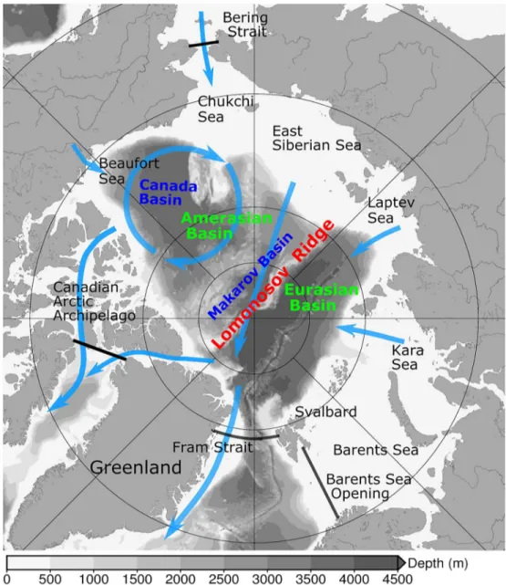
Figure 1. Schematic of the Pan-Arctic surface freshwater circulation (blue arrows). The background gray color shows bottom bathymetry. The Arctic Ocean domain studied in this study is indicated by black lines at the four Arctic gateways.
Journal of Geophysical Research: Oceans
of freshwater in the Arctic Ocean through changing freshwater pathways (Morison et al., 2012; Timmermans et al., 2011).
As Arctic FWC has a long memory of wind forcing, the responses of FWC to different SLP modes over the Arctic Ocean can be used to reconstruct Arctic FWC changes (Johnson et al., 2018; Marshall et al., 2017). The related idea is to obtain a function quantifying the response of the FWC to a step change in SLP, and then convolve the response function with a time series of SLP forcing to reconstruct or predict FWC variability. It is found that there is qualitative agreement among Coupled Model Inter- comparison Project Phase 5 models that a step change to a more anticyclonic Arctic Oscillation (AO) leads to an increase in Arctic FWC, but the models differ widely in the degree to which the response functions can explain Arctic FWC changes (Cornish et al., 2020). In particular, the amplitude of the response of Arctic FWC to a more anticyclonic AO is significantly different among the models. There- fore, process-understanding oriented studies are still required to unravel factors and processes that can influence ocean responses to winds.
Sea ice can modulate the ocean surface stress (e.g., Martin et al., 2014), thus influencing the upper ocean circulation and freshwater spatial distribution (Wang, Wekerle, et al., 2019). Arctic sea ice has undergone a sig- nificant decline over the satellite era (Comiso et al., 2017; Kwok, 2018). The Arctic sea ice decline over the pe- riod 2001–2015 caused pronounced redistribution of freshwater in the Arctic Ocean via strengthening surface Ekman transport: more freshwater was accumulated into the Amerasian Basin (AB), while the FWC in the Eurasian Basin (EB, see Figure 1 for Arctic geographical features) was reduced owing to increasing occupa- tion of Atlantic-origin water and decreasing occupation of Pacific-origin water (Wang, Wekerle, et al., 2019).
Although the Arctic total FWC is not significantly altered by the sea ice decline because the opposite changes of the FWC in the two basins largely compensate each other, regionally the upper ocean salinity, circulation and surface MLD are changed significantly by the sea ice decline. Observational and modeling studies also suggest that sea ice acts as a surface drag to hinder accumulation of freshwater in the Beaufort Gyre despite anticyclonic winds because ocean surface velocities approach or may even exceed those of sea ice when FWC increases in the Beaufort Gyre (Dewey et al., 2018; Meneghello et al., 2018; Wang, Marshall, et al., 2019).
This study aims to improve the understanding on the impact of sea ice decline on the Arctic FWC, SSH and upper ocean circulation. Their responses to the wind variability associated with different atmospheric modes and the impact of Arctic sea ice decline on the responses will be investigated. Ocean-sea ice simu- lations are carried out with wind forcing perturbed relative to a control simulation. Two historical periods, the 1980s and 2010s, are used in order to elucidate the impact of sea ice states. The focus is not only on the Arctic total FWC, but also on the freshwater distribution in the Arctic Ocean and regional changes in SSH and surface ocean circulation.
I describe the model configurations and methodology in Section 2, present the results in Section 3, discuss possible implications of the methodology in Section 4, and then summarize the study in Section 5.
2. Model Setup and Method
I employed the Finite Element Sea-ice Ocean Model (FESOM 1.4, Q. Wang et al., 2014) in this study. FES- OM 1.4 is a global ocean general circulation model discretized on unstructured triangular meshes for both its ocean (Danilov et al., 2004; Wang et al., 2008) and sea ice components (Danilov et al., 2015). The model supports multiresolution global simulations with model resolution coarsened outside regions of interest, so the overall computational cost can be reduced to allow for longer high-resolution simulations with available computing resources.
In the sea ice model, an updated version of the elastic-viscous-plastic (EVP, Hunke & Dukowicz, 1997) sea ice rheology is used (Danilov et al., 2015). The sea ice thermodynamics follow Parkinson and Washing- ton (1979). FESOM can reasonably simulate Arctic sea ice concentration, thickness and small scale linear kinematic features at the scale of the applied model resolution in comparison with other state-of-the-art global ocean models (Wang, Danilov, et al., 2016; Wang, Ilicak, et al., 2016). In the ocean model component, diapycnal mixing and ocean viscosity are parameterized with the K-profile parameterization scheme (Large et al., 1994) and Smagorinsky viscosity (Smagorinsky, 1963) in a biharmonic form, respectively. Eddy dif-
10.1029/2020JC016886
fusivity is scaled with local horizontal resolution as suggested by Wang et al. (2014). The model has an ac- ceptable representation of the Arctic Ocean major circulation and the recent increase in Arctic and Beaufort Gyre FWC (Wang, Wekerle, Danilov, Koldunov, et al., 2018; Wang, Wekerle, Danilov, Wang, & Jung, 2018;
Wang, Wekerle, et al., 2019). A variable-resolution mesh with horizontal resolution of 1° in most parts of the global ocean is used in this study. The resolution is refined to 24 km north of 45°N and further refined to 4.5 km in the Arctic Ocean. The model grid has a vertical spacing of 10 m in the upper 100 m and coarser resolution downward, with 47 z-levels in total.
A control simulation was carried out from 1958 to 2019 driven by the JRA55-do (Tsujino et al., 2018) at- mosphere reanalysis fields and monthly river runoff climatology. The simulation started from the PHC 3 climatology (Steele et al., 2001) and climatological sea ice derived from a previous simulation. Two sets of 10-year-long perturbation experiments were performed starting from the control run results in 1980 and 2010, respectively. In these experiments, wind forcing was perturbed with some anomalies for the calcu- lation of ocean and sea ice surface stress. Wind anomalies associated with three major Arctic atmospheric modes were used.
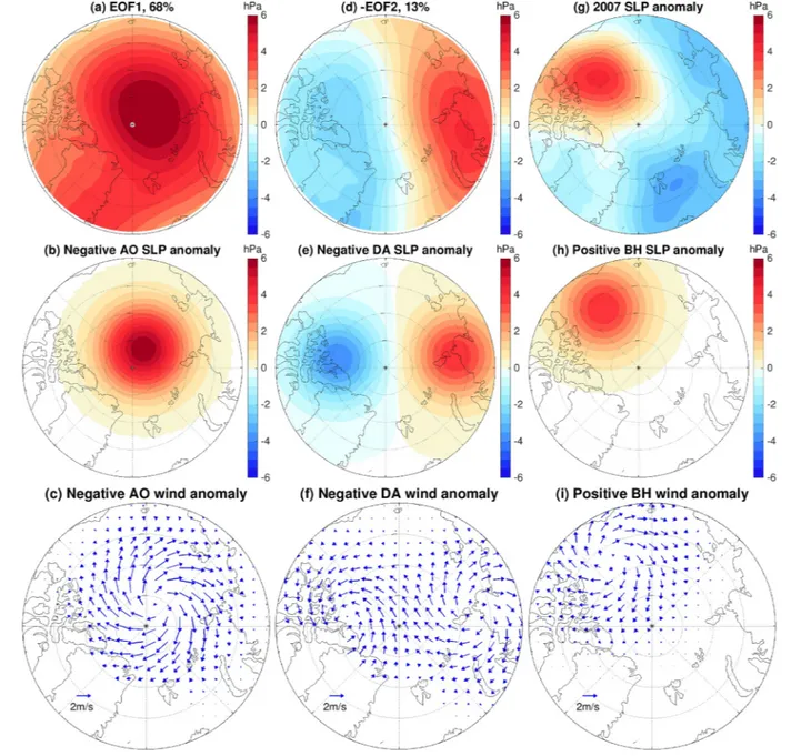
The first two empirical orthogonal functions (EOF) of monthly SLP (north of 70°N for the purpose of this work, seasonal cycle removed) of the JRA55-do data for the period 1980–2019 are shown in Figures 2a and 2d, respectively. EOF1 resembles the negative, anticyclonic AO phase (Thompson &
Wallace, 1998), and explains 68% of the SLP variability. EOF2 explains 13% of the SLP variability and represents the Arctic Dipole Anomaly (DA, Wu et al., 2006). The negative value of EOF2 is shown in Figure 2d, corresponding to the negative phase of the DA. I will consider these two leading modes in perturbation experiments. In addition, I will explore the impact of the BH SLP, which was mainly in a positive phase and caused a significant increase in FWC in the Beaufort Gyre in the early 21st century (e.g., Proshutinsky et al., 2019; Wang, Wekerle, Danilov, Wang, & Jung, 2018; Zhang et al., 2016). The 2007 SLP anomaly depicts the pattern of the BH in a strongly positive phase (Figure 2g). For the pertur- bation experiments, wind anomalies associated with three idealized SLP anomalies are used to represent the three atmospheric modes described above: AO (Figures 2b and 2c), DA (Figures 2e and 2f), and BH (Figures 2h and 2i). The BH anomalies are the same as the BH forcing used in Marshall et al. (2017).
Using the idealized wind anomalies for the purpose of this study allows to focus on the impacts of major atmospheric modes themselves without being bothered by small details; Similar ideas to employ ideal- ized wind perturbations were used in other Arctic Ocean studies (e.g., Muilwijk et al., 2019). The im- pacts of both negative and positive phases of the three atmospheric modes will be investigated through perturbation experiments. For two periods (1980s and 2010s), a total of 12 perturbation experiments were performed.
The response of Arctic liquid FWC to wind perturbations will be studied in this paper. The vertically in- tegrated liquid FWC is defined as FWC 0D(Sref S S dz, where S is salinity, S) / ref ref = 34.8 psu is the reference salinity and D is the isohaline depth of S = Sref. Volumetric FWC is obtained by integrating the vertically integrated FWC laterally. Both the FWC in the Arctic Ocean and the FWC in the Arctic Basin will be analyzed. In this paper, the Arctic Ocean refers to the Arctic region enclosed by the four Arctic gateways (Fram Strait, Barents Sea Opening, Bering Strait and Canadian Arctic Archipelago [CAA]), while the Arctic Basin refers to the central area of the Arctic Ocean with bottom topography deeper than 500 m, including the EB and AB (Figure 1). The EB and AB are separated by Lomonosov Ridge.
3. Results
3.1. Control Run Results
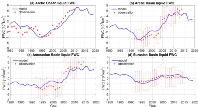
The control run reproduces the observed changes in Arctic liquid FWC well over the last few decades (Fig- ure 3). Observations indicate that the Arctic liquid FWC had an upward trend starting from mid-1990s to at least mid-2010s, with a FWC increase of about 11, 000 km3 (Polyakov et al., 2013; Rabe et al., 2014) (Fig- ures 3a and 3b). The model reasonably simulates the observed FWC increase. The increasing trend of the Arctic FWC is mainly attributed to the trend in the AB (Figure 3c). The trend in the AB is largely captured by the model in most of the years over the observational period, with the simulated variation within the
Journal of Geophysical Research: Oceans
observational uncertainty range. In the EB, the FWC has a weak increasing trend from mid-1990s to mid- 2000s and a weak decreasing trend afterward, which are consistently simulated by the model (Figure 3d).
The model also has a good representation of the declining trend and interannual variability of both Arctic sea ice volume and summer sea ice extent in comparison with the PIOMAS result (Schweiger et al., 2011) and the satellite observations (Fetterer et al., 2017) (Figure 4). The declining trend of Arctic annual mean sea ice volume is −3.1 × 10³ km3/decade (p < 0.01) and −2.5 × 10³ km3/decade (p < 0.01) in the PIOMAS reanalysis and the control run, respectively. Their correlation after detrending is 0.72 (p < 0.01). The de- clining trend of Arctic September sea ice extent is −0.82 million km2/decade (p < 0.01) and −0.65 million km2/decade (p < 0.01) in the satellite observations and the control run, respectively. Their correlation after
10.1029/2020JC016886
Figure 2. (a) The first empirical orthogonal function (EOF) of sea level pressure (SLP, north of 70°N) for the period 1980–2019. It resembles the pattern of the negative, anticyclonic Arctic Oscillation (AO) phase. (b) Idealized SLP anomaly representing negative AO and (c) the associated wind anomaly. (d) The second EOF of SLP. The negative EOF2 is shown, which corresponds to the negative phase of the Arctic Dipole Anomaly (DA). (e) Idealized SLP anomaly representing negative DA and (f) the associated wind anomaly. (g) 2007 SLP anomaly relative to the mean over 1980–2019. It shows a strong positive Beaufort High SLP anomaly. (h) Idealized SLP anomaly representing positive BH anomaly and (i) the associated wind anomaly. BH, Beaufort High.
detrending is 0.82 (p < 0.01). The two time periods that will be investigated in this study correspond to the decades with highest (1980s) and lowest (2010s) sea ice thickness and concentration in the satellite era.
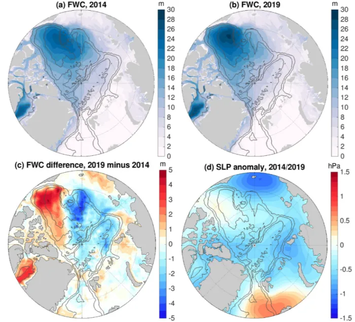
As mentioned in the introduction, it is important to know the spatial distribution of freshwater in the Arctic Ocean. For example, there is a significant regional increase in the FWC in the Beaufort Gyre region from 2014 to 2019 (Figure 5), although the Arctic total FWC does not increase in this period (Figure 3a). Freshwater is accumulated in the Beaufort Gyre from 2014 to 2019, with the Beaufort Gyre center moving eastward (Figures 5a–5c), opposite to the westward movement during preceding years that was reported by Regan et al. (2019). Consistent with the higher SLP in the southeastern Canada Basin and lower SLP outside (Figure 5d), which drives Ekman convergence, FWC increases in the southeastern Canada Basin and north of the CAA, and decreases in other parts of the AB and in the EB (Figure 5c). The positive and negative FWC changes in the AB largely compensate each other, so the FWC integrated in the AB does not change much (Figure 3c). Calculating only the total FWC in the Arctic does not tell the interesting and important changes in the freshwa- ter spatial distribution. In the following, we will investigate the response of Arctic FWC and the freshwater spatial distribution as well to different atmospheric modes and sea ice states.
3.2. Response of FWC to Atmospheric Modes
The response of Arctic FWC to different atmospheric modes in the 2010s period will be investigated in this section. The changes in ocean surface Ekman transport (calculated from ocean surface stress) induced by the wind perturbations of negative AO, negative DA and positive BH modes are shown in Figures 6a, 6c, and 6e. As expected from the applied wind perturbations (Figure 2), the negative (anticyclonic) AO leads to Ekman convergence toward the central Arctic, the negative DA (high SLP over Figure 3. Liquid freshwater content (FWC, 103 km3) anomalies in the (a) Arctic Ocean, (b) Arctic Basin (Amerasian Basin [AB] plus Eurasian Basin [EB]), (c) AB and (d) EB. The model results are shown with blue curves and observations are shown with red dots. Observational data in (a) and (b–d) are described in Polyakov et al. (2013) and Rabe et al. (2014), respectively. The observational error bars are shown in (b–d).
Figure 4. (a) Arctic annual mean sea ice volume from the control run and the Pan-Arctic Ice Ocean Modeling and Assimilation System (PIOMAS) result (Schweiger et al., 2011). (b) Arctic September sea ice extent from the control run and the National Snow and Ice Data Center (NSIDC) satellite observation (Fetterer et al., 2017). The anomalies are relative to the respective mean values, and the mean values are shown in the legends.
Journal of Geophysical Research: Oceans
the Eurasian continental shelf and low SLP north of CAA and Greenland) leads to Ekman convergence toward the central Eurasian coast and Ekman divergence from north of the CAA, and the positive (anticy- clonic) BH leads to Ekman convergence toward the Beaufort Gyre (Figures 6a, 6c, and 6e). Their opposite phases cause similar Ekman transport anomalies in opposite directions (not shown).
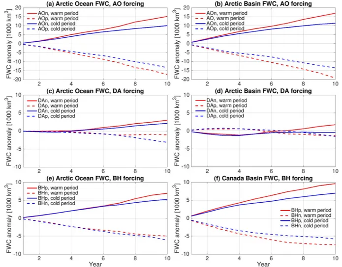
The AO perturbation causes significant changes in the amount of freshwater in the EB, Makarov Basin and the western Canada Basin (Figures 7a and 7b). In these areas, the FWC increases in response to changes in the Ekman transport under negative AO perturbation and decreases under positive AO perturbation. The FWC in most areas of the continental shelf (including eastern Beaufort Sea, north of CAA and Greenland, and most of the Eurasian continental shelf) and in the export gateways to the North Atlantic (CAA and western Fram Strait) has changes with signs opposite to the central Arctic. Integrated over the Arctic Ocean, the FWC increases persistently under the negative AO perturbation and decreases persistently under the positive AO perturbation over the 10 years period (red curves in Figure 8a). The amplitudes of the changes in the Arctic FWC are similar between the negative and positive AO modes. The changes in the Arctic Basin (EB plus AB) are slightly larger than those of the Arctic total FWC (Figure 8b). This is related to the fact that
10.1029/2020JC016886
Figure 5. (a) Freshwater content (FWC, m) in 2014 from the control run. (b) The same as (a) but for 2019. (c) The FWC difference between 2019 and 2014. (d) The sea level pressure (SLP) anomaly in 2014–2019 relative to the 1980–2019 mean. The black contour lines indicate the 500, 2,000, and 3,500 m isobaths.
the changes in the FWC over Arctic continental shelves caused by the AO perturbations are opposite to the changes in the central basin (Figures 7a and 7b).
The DA perturbation causes FWC to change with opposite signs between two regions: the first region con- sists of the eastern EB, western AB, and their adjacent shelf seas (Laptev and East Siberian seas); the other region includes north of CAA and Greenland, and the Barents Sea (Figures 7c and 7d). A negative DA raises the FWC in the first region while a positive DA reduces it; The opposite happens in the second region. In comparison to the impact of the AO perturbation, the DA perturbation does not significantly change the to- tal FWC in the Arctic Ocean and in the Arctic Basin (Figures 8c and 8d), as the opposite changes in different regions largely compensate each other (Figures 7c and 7d). Therefore, the DA perturbation mainly drives redistribution of freshwater within the Arctic Ocean.
The FWC in the Canada Basin becomes higher with a positive BH perturbation and lower with a negative one (Figures 7e and 7f). In the EB and part of the Makarov Basin adjacent to the Lomonosov Ridge, the FWC has relatively weaker changes with a sign opposite to that in the Canada Basin. The total FWC in the Canada Basin increases persistently under the positive BH perturbation and decreases under the negative BH perturbation (Figure 8f). The changing rates become smaller with time as expected from the feedback effect of ice-ocean stress coupling and the effect of eddy dissipation (Dewey et al., 2018; Manucharyan &
Spall, 2016; Meneghello et al., 2018; Wang, Marshall, et al., 2019), although the FWC in the Canada Basin does not reach an equilibrium state within the simulation period. The changes in the Arctic total FWC are smaller than those in the Canada Basin (Figures 8e and 8f) because of opposite changes outside the Canada Basin (Figures 7e and 7f).
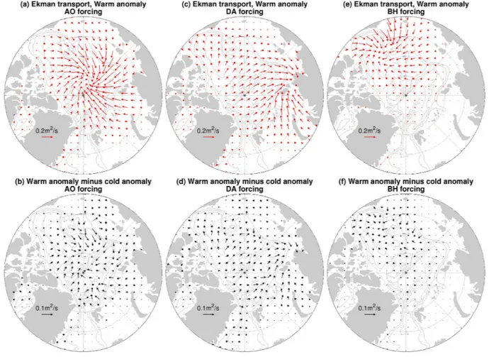
Figure 6. (a) Surface Ekman transport anomaly in the perturbation experiment with the negative Arctic Oscillation (AO) forcing relative to the control simulation for the warm (2010s) period. (b) The difference of Ekman transport anomalies induced by negative AO forcing between the warm and cold (1980s) periods. (c), (d) The same as (a) and (b), but for the negative Dipole Anomaly (DA) forcing. (e), (f) The same as (a) and (b), but for the positive Beaufort High (BH) forcing. The gray contour lines indicate the 500, 2,000, and 3,500 m isobaths.
Journal of Geophysical Research: Oceans
3.3. Impact of Sea Ice Decline on FWC
In this section, the impact of sea ice decline on the response of the Arctic FWC to different atmospheric modes will be elucidated by comparing the two sets of perturbation experiments over different periods.
Sea ice is thicker and more compact in the cold scenario (1980s) than in the warm scenario (2010s). As a consequence, the ocean surface Ekman transport anomalies in the warm scenario are stronger than in the cold scenario for all the atmospheric modes (Figures 6b, 6d, and 6f). The Ekman transport in the warm sce- nario is considered stronger because the differences of Ekman transport anomalies between the two periods (warm scenario minus cold scenario) are largely aligned with the anomalies themselves (comparing the bottom row with the upper row in Figure 6).
The response of FWC in the Arctic Ocean to the AO perturbation in the cold scenario is qualitatively similar to that in the warm scenario (Figures 9a and 9b vs. Figures 7a and 7b). Quantitatively, however, the FWC changes in the Arctic Basin are weaker in the cold scenario. In addition, the area in the Arctic Basin with positive (negative) FWC anomalies induced by the negative (positive) AO mode is smaller in the cold sce- nario. Integrated over the Arctic Basin or over the whole Arctic Ocean, the amplitude of the FWC anomaly at the end of the simulations is 40%–50% higher in the warm scenario than in the cold scenario (Figures 8a and 8b).
The negative and positive changes of FWC in the Arctic Basin with the DA perturbation are confined to the two regions roughly separated by the 0°/180° longitude line (the Eurasian and Amerasian sectors) in the cold scenario (Figures 9c and 9d). In the warm scenario, the changes are less confined spatially (Fig- ures 7c and 7d). In particular, the positive anomaly driven by the negative DA mode occupies the eastern EB and western AB as well in the warm scenario (Figure 7c). In both the cold and warm scenarios, the DA
10.1029/2020JC016886
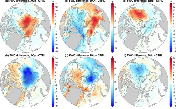
Figure 7. (a) Anomaly of the liquid freshwater content (FWC, m) in the perturbation experiment with negative Arctic Oscillation (AO) forcing in 2019 (the last year of the warm period) relative to the control simulation. (b) The same as (a), but for the positive AO forcing case. (c and d) The same as (a) and (b), but for the cases with Dipole Anomaly (DA) forcing. (e and f) The same as (a) and (b), but for the cases with Beaufort High (BH) forcing. The results for 1989 (the last year of the cold period) are shown in Figure 9. Note that the color range in (c and d) is different from that in other panels. The black contour lines indicate the 500, 2,000, and 3,500 m isobaths. The blue lines in (e) indicate the Canada Basin, defined as within the longitude range 130°W to 180°W and latitude range 70°N to 85°N, and where bathymetry is deeper than 500 m.
perturbation does not significantly change the total FWC integrated over the Arctic Basin and Arctic Ocean in comparison with the other two atmospheric modes (Figures 8c and 8d). The DA perturbation leads to significant changes in the FWC in some of the shelf seas (Figures 9c and 9d), which is due to the impact of winds on sea ice transport and thermodynamics (see Section 3.5 for further discussion).
In the cold scenario, the spatial patterns of the changes in FWC induced by the BH perturbations are similar to those in the warm scenario (Figures 9e and 9f vs. Figures 7e and 7f). However, the amplitude of the FWC anomalies in the Canada Basin is weaker in the cold scenario. Furthermore, in the cold scenario, the FWC in the Makarov Basin changes as in the Canada Basin: positively with the positive BH mode and negatively with the negative BH mode. In the warm scenario, in contrast, the sign of the FWC anomaly in most of the Makarov Basin is opposite to that in the Canada Basin. This difference between the two scenarios is due to the stronger Ekman convergence to, or divergence from, the Canada Basin in the warm scenario. Integrated over the whole Arctic Ocean, the changes in the total FWC with the BH perturbation are the same between the two scenarios over the first five model years (Figure 8e). Although some difference between the two scenarios appears afterward, there is no agreement for the two BH modes on whether the changes in Arctic FWC are larger in the warm scenario. However, the total FWC in the Canada Basin consistently changes more strongly in the warm scenario for both the positive and negative modes (by about 40%, Figure 8f).
Figure 8. (a) Anomaly of Arctic total liquid freshwater content (FWC, 103 km3) in the perturbation experiments with Arctic Oscillation (AO) forcing relative to the control simulation. (b) The same as (a), but for the FWC in the Arctic Basin including the Amerasian and Eurasian basins. (c and d) The same as (a) and (b), but for the cases with Dipole Anomaly (DA) forcing. (e) The same as (a), but for the cases with Beaufort High (BH) forcing. (f) The same as (e), but for the FWC in the Canada Basin, which is indicated by blue lines in Figure 7e.
Journal of Geophysical Research: Oceans
3.4. Variability of SSH and Ocean Circulation
The changes in the Arctic SSH closely follow those of FWC (cf. Figures 10 and S1) due to the dominant ha- losteric effect. In the control run, the anticyclonic circulation associated with the high sea level is centered around the Beaufort Gyre and confined to the AB, while a weak cyclonic circulation is present in the EB.
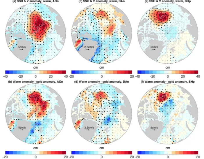
In the AO perturbation experiments, the SSH increases (decreases) in most parts of the Arctic Basin with the negative (positive) AO perturbation (Figures 10a and 10b). With the negative AO mode, the anticyclonic circulation intensifies and expands into the EB, and the cyclonic circulation in the EB is finally eliminated after the negative AO perturbation is enforced for a sufficiently long time (cf. Figure 10a and the control run result on top of Figure 10). With the positive AO mode, the anticyclonic circulation shrinks to a very small area in the southeastern Canada Basin, and the cyclonic circulation not only strengthens in the EB, but also expands to the Makarov Basin and northwestern Canada Basin (Figure 10b). The DA perturbation causes the SSH and upper ocean circulation to change as well (Figures 10c and 10d). Although the location of the front between the anticyclonic and cyclonic circulations is not significantly changed by the DA per- turbation, its strength is weakened (strengthened) by the negative (positive) DA mode. The most significant impact of the BH perturbation is in the Canada Basin (Figures 10e and 10f). The positive (negative) BH mode strengthens (weakens) the Beaufort Gyre circulation and increases (decreases) the sea level in the Canada Basin.
To illustrate the impact of sea ice decline on the response of SSH and ocean circulation to winds, the anoma- lies of SSH and upper ocean velocity induced by wind perturbations in the warm scenario and the differenc- es of the anomalies between the warm and cold scenarios are shown in Figure 11. For brevity, results from only one phase of each atmospheric mode are shown. The anomalies of SSH are associated with the anom- alies of FWC (cf. Figures 11a, 11c, and 11e and Figures 7a, 7c, and 7e), and the upper ocean velocity anom- alies are mainly determined by the SSH anomalies (that is, surface geostrophic velocity). In comparison
10.1029/2020JC016886
Figure 9. (a) Anomaly of liquid freshwater content (FWC, m) in the perturbation experiment with negative Arctic Oscillation (AO) forcing in 1989 (the last year of the cold period) relative to the control simulation. (b) The same as (a), but for the positive AO forcing case. (c and d) The same as (a) and (b), but for the cases with Dipole Anomaly (DA) forcing. (e and f) The same as (a) and (b), but for the cases with Beaufort High (BH) forcing. The results for 2019 (the last year of the warm period) are shown in Figure 7. Note that the color range in (c and d) is different from that in other panels. The black contour lines indicate the 500, 2,000, and 3,500 m isobaths.
with the cold scenario, the warm scenario allows for stronger responses of the SSH and ocean circulation to winds, especially for the AO and BH perturbations. With the negative AO mode, the SSH in the eastern EB and northwestern AB increases more in the warm scenario by up to nearly 100% in some places (the SSH anomaly in the warm scenario is nearly twice the difference of the anomalies between the warm and cold scenarios in those areas), leading to stronger anticyclonic circulation in these areas (Figure 11b). With the positive BH mode, the SSH rise in the western Canada Basin is also larger by up to about 100% in the warm scenario than in the cold scenario (Figure 11f). The warm scenario allows for a stronger anticyclonic circulation in the western Canada Basin under the forcing of the positive BH mode. In the meanwhile, the Figure 10. (a) Sea surface height (SSH, color patches) and upper 150 m velocity (arrows) in the perturbation experiment with negative Arctic Oscillation (AO) forcing in 2019. (b) The same as (a), but for the case with positive AO forcing. (c and d) The same as (a and b), but for the cases with Dipole Anomaly (DA) forcing. (e and f) The same as (a and b), but for the cases with Beaufort High (BH) forcing. For comparison, the result in the control simulation is shown in the top row. The gray contour lines indicate the 500, 2,000, and 3,500 m isobaths.
Journal of Geophysical Research: Oceans
difference of the SSH anomalies in the Makarov Basin between the two scenarios is negative (warm scenar- io minus cold scenario), consistent with the different changes in the FWC in this basin in the two climate scenarios (Figures 7e and 9e). With the DA perturbation, a clear difference of SSH and ocean circulation anomalies between the two scenarios is also present (e.g., in the western Canada Basin) but it is less pro- nounced than with the other two atmospheric modes (Figure 11d), as expected from the smaller difference in the FWC anomalies presented above.
Sea ice can influence the FWC through the ice-ocean stress feedback, especially in the Beaufort Gyre re- gion (Dewey et al., 2018; Meneghello et al., 2018; Wang, Marshall, et al., 2019). If the role of this feedback changes with sea ice decline, the effect is already contained in the impacts of sea ice decline identified in this study. One can quantify this component of the effect numerically using the method proposed in Wang, Marshall, et al. (2019), which is beyond the scope of the current study.
3.5. Contribution from Changes in Sea Ice Thermodynamics
The DA perturbation induces FWC changes in the East Siberian and Laptev seas with amplitudes compa- rable to those in the Arctic Basin in the cold scenario (Figures 9c and 9d). To better understand the reason for these changes, an additional sensitivity experiment was performed. This experiment is the same as the
10.1029/2020JC016886
Figure 11. (a) Anomalies of sea surface height (SSH, color patches) and upper 150 m velocity (arrows) in the perturbation experiment with negative Arctic Oscillation (AO) forcing in 2019 (the last year of the warm period) relative to the control simulation. (b) The same as (a), but for the difference of the anomalies between 2019 and 1989 (the last year of the cold period). (c and d) The same as (a and b), but for the cases with negative Dipole Anomaly (DA) forcing. (e and f) The same as (a and b), but for the cases with positive Beaufort High (BH) forcing. Note that different color ranges and vector scales are used. The gray contour lines indicate the 500, 2,000, and 3,500 m isobaths.
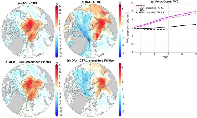
perturbation experiment with negative DA perturbation in the cold scenario, except that the ocean surface freshwater flux was prescribed with values obtained from the control run. In this simulation, the changes of FWC in the East Siberian and Laptev seas are much weaker than in the original perturbation experiment (cf. Figures 12c and 12d). In addition, some difference between these two experiments is also found in the Arctic Basin and close to Greenland. Therefore, the wind perturbation influences the regional FWC not only through changing the ocean surface stress, but also through transporting sea ice and then changing sea ice thermodynamics (freshwater loss and gain due to sea ice freezing and melting). The negative DA mode (Figure 2f) reduces sea ice export from the Laptev and East Siberian seas to the Arctic Basin and from the Arctic interior to north Greenland and Fram Strait (Figure S2), as also suggested in previous studies (Wang et al., 2009; Wu et al., 2006), which reduces sea ice freezing and brine rejection in the upstream regions, thus increasing the FWC there. The fact that the impact of the DA perturbation on the FWC in the East Siberian and Laptev seas is stronger in the cold period reveals that the sea ice advection effect is more pronounced in the cold period, when sea ice is thicker and its volume transport is larger.
The above results indicate that the impact of the DA perturbation on regional FWC through changing sea ice thermodynamics is not negligible compared to the impact through changing the ocean surface stress. A similar sensitivity experiment was performed for the negative AO perturbation case. In this case, prescrib- ing surface freshwater flux does not change the FWC significantly compared to the overall FWC anomaly induced by the wind perturbation (cf. Figures 12a and 12b), which proves that the impact through changing the ocean surface stress plays a dominant role with the AO forcing. The relative importance of the two processes through which winds influence the FWC is also seen in the total FWC integrated over the Arctic Ocean (Figure 12e). With the negative AO perturbation, the Arctic total FWC has a strong increase, a very small part of which is due to changes in sea ice thermodynamics. With the negative DA perturbation, the Arctic total FWC has a relatively small increase, which is mainly due to changes in sea ice thermodynamics.
Figure 12. (a) Anomaly of freshwater content (FWC, m) in the perturbation experiment with negative Arctic Oscillation (AO) forcing in 1989 (the last year of the 10-year simulations) relative to the control simulation. (b) The same as (a), but for the modified perturbation experiment with negative AO forcing, in which the ocean surface freshwater fluxes are prescribed with values obtained from the control simulation. (c and d) The same as (a and b), but for the cases with negative Dipole Anomaly (DA) forcing. (e) Time series of the anomalies of the Arctic total FWC (103 km3) in the four simulations shown in (a–d). The black contour lines in (a–d) indicate the 500, 2,000, and 3,500 m isobaths.
Journal of Geophysical Research: Oceans
As the response of sea ice thermodynamics to wind perturbations can be very nonlinear and dependent of the state of sea ice locally, it is unsurprising that the response of the Arctic FWC is not symmetric between the negative and positive phases of the DA forcing (Figure 8c). The impact of different atmospheric modes on sea ice advection and thermodynamics is beyond the scope of this study and is thus not explored in detail here.
4. Discussion
Two sets of perturbation experiments over two different periods (1980s and 2010s) were performed in order to understand the impact of sea ice decline on the response of Arctic FWC and ocean circulation to wind perturbations as presented above. Between these two sets of experiments, the ocean salinity is different at the beginning of the simulations. The Arctic FWC at the beginning of the 2010s is about 5 × 10³ km3 higher than that at the beginning of the 1980s (Figure 4a), about 6% of the Arctic total liquid FWC. With a fresher ocean, even the same total Ekman volume transport can carry a larger amount of freshwater. Does the difference in the initial salinity significantly contribute to the difference in the ocean response to wind perturbations between the two sets of experiments described in Section 3.3?
To answer this question, a passive tracer is introduced in both the control run and the run with the negative AO perturbation in the period of the 1980s. The initial value of the passive tracer is set to the salinity value at the beginning of the 2010s simulations, that is, the salinity in the control run at the end of 2009. The passive tracer receives the same surface fluxes as ocean salinity does during the simulations. If the initial salinity does not significantly influence the response of the Arctic FWC to the wind perturbation, the FWC difference between these two simulations calculated from the passive tracer should be close to the FWC difference calculated from ocean salinity. Indeed, the FWC differences calculated from the two approaches are similar for both the total Arctic Ocean and the Arctic Basin (Figures 13a and 13b), indicating a relatively small impact from the difference of initially available freshwater in comparison with the impact of sea ice
10.1029/2020JC016886
Figure 13. (a and b) Impact of initial ocean salinity. (a) Anomaly of Arctic total liquid freshwater content (FWC, 103 km3) in the experiments with negative Arctic Oscillation (AO) forcing relative to the control simulation. (b) The same as (a), but for the FWC in the Arctic Basin including the Amerasian and Eurasian basins. The results reveal that the difference in the ocean salinity (available freshwater) at the beginning of the two periods plays a less important role than the difference in the sea ice condition. (c and d) The same as (a and b), but for the impact of background winds. The results reveal that the difference in the background winds between the two periods plays a minor role in the response of the FWC to the wind perturbation.
decline. I hypothesize that this is because the difference of the initial FWC between the two periods is rela- tively small compared to the Arctic total FWC.
The wind forcing in the control run is also different between the two periods. Does the difference in the background winds significantly influence the response of the Arctic FWC to the applied wind perturbation?
To answer this question, two additional simulations were carried out. They are the same as the control run and the run with negative AO perturbation in the period of the 1980s, respectively, except that background winds from the 2010s are instead used. As shown in Figures 13c and 13d, the FWC anomaly between these two simulations is nearly the same as that obtained by using background winds from the 1980s, indicating that the difference in the background winds between the two periods does not have a large impact.
5. Summary
I answered three questions in this study: (1) Does sea ice decline influence the response of Arctic freshwa- ter content (FWC) to variations in the atmospheric circulation?; (2) Is the impact of sea ice decline on the response different for different atmospheric modes?; (3) Does sea ice decline strengthen the decadal varia- bility of Arctic FWC, sea level and upper ocean circulation? I found that the answers to these questions are affirmative.
To answer these questions, a model configuration based on FESOM was employed, which can reasonably reproduce the observed variability and trends of Arctic FWC and sea ice over the past decades. Perturbation experiments were performed with wind forcing perturbed with three different Arctic sea level pressure (SLP) modes: Arctic Oscillation (AO), Dipole Anomaly (DA) and Beaufort High (BH). Perturbations with both negative and positive phases of these modes were considered. To understand the impact of Arctic sea ice decline, the perturbation experiments were performed over two periods separately (1980s with thicker and more compact sea ice, and 2010s with thinner and looser sea ice). The impacts of sea ice decline were identified by comparing the responses of FWC, sea surface height (SSH) and ocean circulation to winds between these two climate scenarios.
A negative AO mode increases FWC and SSH in the Arctic Basin and leads to weaker opposite changes over Arctic continental shelves; A positive AO mode has opposite impacts. Winds drive the redistribution of freshwater, thus changing the SSH pattern (the halosteric effect). The surface geostrophic currents change accordingly. The changes in geostrophic currents could also further impact the freshwater distribution, but the spatial pattern of the changes in FWC indicates that the Ekman transport associated with the wind perturbation plays the leading role. A negative AO mode intensifies the anticyclonic circulation and can ex- pand it to the Eurasian Basin (EB) after the mode is active for some years, while a positive AO mode causes the anticyclonic circulation to shrink and can expand the cyclonic circulation from the EB to the Amerasian Basin (AB). The location of the front between the anticyclonic and cyclonic circulations shifts accordingly.
These responses are stronger in the warm scenario than in the cold scenario. The amplitudes of the response of SSH and surface currents to the AO perturbation in the warm scenario can reach nearly twice those in the cold scenario in some places. The changes in Arctic total FWC induced by the AO modes are 40%–50%
larger in the warm scenario than in the cold scenario.
A positive BH mode increases FWC and SSH in the Canada Basin and leads to weaker opposite changes in the EB and continental shelves around the AB; A negative BH mode causes opposite changes. The anticy- clonic circulation in the Canada Basin is intensified by the positive BH mode and weakened by the negative BH mode. These responses are stronger in the warm scenario than in the cold scenario, especially in the western Canada Basin, where the amplitudes of the changes in SSH and surface velocity in the warm sce- nario are about twice those in the cold scenario. The changes in the total FWC in the Canada Basin with the BH perturbation are about 40% stronger in the warm scenario.
The DA perturbation does not significantly change the Arctic total FWC, but it does change the spatial dis- tribution of freshwater in the Arctic Ocean. In the cold scenario, a negative DA mode raises FWC in the EB and reduces FWC in the AB, while the opposite happens with a positive DA mode. In the warm scenario, the changes in FWC are less regular in space. For example, the FWC increases offshore the Chukchi Sea with the negative DA mode in the warm scenario, opposite to that in the cold scenario. Winds can influence the
Journal of Geophysical Research: Oceans
liquid FWC through changing sea ice transport and thus thermodynamics. With the DA perturbation, this effect is not negligible compared with the impact through changing ocean surface stress, in contrast to the case with the AO perturbation.
Considering that AO is the leading mode of the Arctic SLP variability and that the BH anomaly drives the variability of the FWC in the central Canada Basin, the largest freshwater reservoir of the Arctic Ocean (Proshutinsky et al., 2009), the findings in this paper indicate that Arctic sea ice decline can strengthen the decadal variability of the Arctic FWC, SSH and surface circulation, both Arctic-wide and regionally. A positive BH anomaly has been driving the increase of Arctic FWC in the early 21st century. Over this period, the sea ice decline increases the FWC in the AB and reduces it in the EB so that the time evolution of the Arctic total FWC is not significantly changed by the sea ice decline (Q. Wang, Wekerle, et al., 2019). This is consistent with the current finding about the impact of sea ice decline on FWC and SSH under the BH perturbation. In some CMIP5 coupled models the linear response of Arctic FWC to AO can well explain the simulated Arctic FWC variability, while it cannot do so in some other models (Cornish et al., 2020). As the response is significantly influenced by sea ice states as found in the current study, it is not surprising that the variability of SLP alone is insufficient for quantitatively explaining the variability of Arctic FWC.
Numerical simulations often have large spread in their sea ice mean states and trends (e.g., Shu et al., 2020;
Wang, Ilicak, et al., 2016), so it can be expected that the response of Arctic FWC to changes in SLP behaves differently in different models.
The findings in this study suggest that sea ice states need to be considered when understanding and pre- dicting changes in Arctic FWC, dynamic sea level and ocean circulation. The increasing vulnerability of the Arctic Ocean to winds due to sea ice decline also implies that extreme marine events (for example, unprecedented high FWC and strong ocean currents) will possibly occur more often in the Arctic Ocean in a warmer climate.
Data Availability Statement
The model data used in figures can be found at http://doi.org/10.5281/zenodo.4079497.
References
Aagaard, K., Swift, J. H., & Carmack, E. (1985). Thermohaline circulation in the Arctic Mediterranean Seas. Journal of Geophysical Re- search, 90, 4833–4846.
Armitage, T., Bacon, S., & Kwok, R. (2018). Arctic sea level and surface circulation response to the Arctic oscillation. Geophysical Research Letters, 45, 6576–6584. https://doi.org/10.1029/2018GL078386
Armitage, T., Bacon, S., Ridout, A., Thomas, S., Aksenov, Y., & Wingham, D. (2016). Arctic sea surface height variability and change from satellite radar altimetry and GRACE, 2003–2014. Journal of Geophysical Research: Oceans, 121, 4303–4322. https://doi.
org/10.1002/2015JC011579
Comiso, J. C., Meier, W. N., & Gersten, R. (2017). Variability and trends in the Arctic sea ice cover: Results from different techniques. Jour- nal of Geophysical Research: Oceans, 122, 6883–6900. https://doi.org/10.1002/2017JC012768
Cornish, S. B., Kostov, Y., Johnson, H. L., & Lique, C. (2020). Response of Arctic freshwater to the Arctic Oscillation in coupled climate models. Journal of Climate, 33, 2533–2555. https://doi.org/10.1175/JCLI-D-19-0685.1
Danilov, S., Kivman, G., & Schröter, J. (2004). A finite-element ocean model: Principles and evaluation. Ocean Modelling, 6, 125–150.
https://doi.org/10.1016/S1463-5003(02)00063-X
Danilov, S., Wang, Q., Timmermann, R., Iakovlev, N., Sidorenko, D., Kimmritz, M., & Schroeter, J. (2015). Finite-Element Sea Ice Model (FESIM), version 2. Geoscientific Model Development, 8, 1747–1761. https://doi.org/10.5194/gmd-8-1747-2015
Dewey, S., Morison, J., Kwok, R., Dickinson, S., Morison, D., & Andersen, R. (2018). Arctic ice-ocean coupling and gyre equilibration ob- served with remote sensing. Geophysical Research Letters, 45, 1499–1508. https://doi.org/10.1002/2017GL076229
Fetterer, F., Knowles, K., Meier, W., Savoie, M., & Windnage, A. K. (2017). Sea ice index, version 3. Boulder, CO: NSIDC: National Snow and Ice Data Center.
Giles, K. A., Laxon, S. W., Ridout, A. L., Wingham, D. J., & Bacon, S. (2012). Western Arctic Ocean freshwater storage increased by wind-driven spin-up of the Beaufort Gyre. Nature Geoscience, 5, 194–197. https://doi.org/10.1038/ngeo1379
Haine, T., Curry, B., Gerdes, R., Hansen, E., Karcher, M., Lee, C., & Woodgate, R. (2015). Arctic freshwater export: Status, mechanisms, and prospects. Global and Planetary Change, 125, 13–35. https://doi.org/10.1016/j.gloplacha.2014.11.013
Hunke, E., & Dukowicz, J. (1997). An elastic-viscous-plastic model for sea ice dynamics. Journal of Physical Oceanography, 27, 1849–1867.
Jahn, A., & Holland, M. M. (2013). Implications of arctic sea ice changes for North Atlantic deep convection and the meridional overturn- ing circulation in CCSM4-CMIP5 simulations. Geophysical Research Letters, 40, 1206–1211. https://doi.org/10.1002/grl.50183 Johnson, H. L., Cornish, S. B., Kostov, Y., Beer, E., & Lique, C. (2018). Arctic Ocean freshwater content and its decadal memory of sea-level
pressure. Geophysical Research Letters, 45, 4991–5001. https://doi.org/10.1029/2017GL076870
Kwok, R. (2018). Arctic sea ice thickness, volume, and multiyear ice coverage: Losses and coupled variability (1958–2018). Environmental Research Letters, 13, 105005. https://doi.org/10.1088/1748-9326/aae3ec
10.1029/2020JC016886
Acknowledgments
This work is supported by the German Helmholtz Climate Initiative REKLIM (Regional Climate Change). The author thanks the two anonymous review- ers and the editor for their helpful comments.
Large, W. G., Mcwilliams, J. C., & Doney, S. C. (1994). Oceanic vertical mixing: A review and a model with a nonlocal boundary-layer parameterization. Reviews of Geophysics, 32, 363–403. https://doi.org/10.1029/94RG01872
Manucharyan, G., & Spall, M. (2016). Wind-driven freshwater buildup and release in the Beaufort Gyre constrained by mesoscale eddies.
Geophysical Research Letters, 43, 273–282. https://doi.org/10.1002/2015GL065957
Marshall, J., Scott, J., & Proshutinsky, A. (2017). “climate response functions” for the Arctic Ocean: A proposed coordinated modelling experiment. Geoscientific Model Development, 10, 2833–2848. http://doi.org/10.5194/gmd-10-2833-2017
Martin, T., Steele, M., & Zhang, J. (2014). Seasonality and long-term trend of Arctic Ocean surface stress in a model. Journal of Geophysical Research: Oceans, 119, 1723–1738. https://doi.org/10.1002/2013JC009425
Meneghello, G., Marshall, J., Timmermans, M., & Scott, J. (2018). Observations of seasonal upwelling and downwelling in the Beaufort Sea mediated by sea ice. Journal of Physical Oceanography, 48, 795–805. https://doi.org/10.1175/JPO-D-17-0188.1
Morison, J., Kwok, R., Peralta-Ferriz, C., Alkire, M., Rigor, I., Andersen, R., & Steele, M. (2012). Changing Arctic Ocean freshwater path- ways. Nature, 481, 66–70. https://doi.org/10.1038/nature10705
Muilwijk, M., Ilicak, M., Cornish, S. B., Danilov, S., Gelderloos, R., Gerdes, R., & Wang, Q. (2019). Arctic Ocean response to Green- land Sea wind anomalies in a suite of model simulations. Journal of Geophysical Research: Oceans, 124, 6286–6322. https://doi.
org/10.1029/2019JC015101
Parkinson, C. L., & Washington, W. M. (1979). A large-scale numerical model of sea ice. Journal of Geophysical Research, 84, 311–337.
Polyakov, I., Bhatt, U., Walsh, J., Abrahamsen, E. P., Pnyushkov, A., & Wassmann, P. (2013). Recent oceanic changes in the Arctic in the context of long-term observations. Ecological Applications, 23, 1745–1764. https://doi.org/10.1890/11-0902.1
Popova, E. E., Yool, A., Coward, A. C., Aksenov, Y. K., Alderson, S. G., de Cuevas, B. A., & Anderson, T. R. (2010). Control of primary production in the Arctic by nutrients and light: Insights from a high resolution ocean general circulation model. Biogeosciences, 7, 3569–3591. https://doi.org/10.5194/bg-7-3569-2010
Proshutinsky, A., & Johnson, M. (1997). Two circulation regimes of the wind-driven Arctic Ocean. Journal of Geophysical Research, 102, 12493–12514.
Proshutinsky, A., Krishfield, R., Timmermans, M.-L., Toole, J., Carmack, E., McLaughlin, F., & Shimada, K. (2009). Beaufort Gyre freshwater reservoir: State and variability from observations. Journal of Geophysical Research, 114, C00A10. https://doi.org/10.1029/2008JC005104 Proshutinsky, A., Krishfield, R., Toole, J. M., Timmermans, M. L., Williams, W., Zimmermann, S., & Zhao, J. (2019). Analysis of the Beaufort Gyre freshwater content in 2003–2018. Journal of Geophysical Research: Oceans, 124, 9658–9689. https://doi.org/10.1029/2019JC015281 Rabe, B., Karcher, M., Kauker, F., Schauer, U., Toole, J. M., Krishfield, R. A., & Su, J. (2014). Arctic ocean basin liquid freshwater storage
trend 1992–2012. Geophysical Research Letters, 41, 961–968. https://doi.org/10.1002/2013GL058121
Regan, H. C., Lique, C., & Armitage, T. W. K. (2019). The Beaufort Gyre extent, shape, and location between 2003 and 2014 from satellite observations. Journal of Geophysical Research: Oceans, 124, 844–862. https://doi.org/10.1029/2018JC014379
Rudels, B., Anderson, L. G., & Jones, E. P. (1996). Formation and evolution of the surface mixed layer and halocline of the Arctic Ocean.
Journal of Geophysical Research, 101, 8807–8821.
Schweiger, A., Lindsay, R., Zhang, J., Steele, M., Stern, H., & Kwok, R. (2011). Uncertainty in modeled Arctic sea ice volume. Journal of Geophysical Research, 116, C00D06. https://doi.org/10.1029/2011JC007084
Shu, Q., Wang, Q., Song, Z., Qiao, F., Zhao, J., Chu, M., & Li, X. (2020). Assessment of sea ice extent in CMIP6 with comparison to observa- tions and CMIP5. Geophysical Research Letters, 47, e2020GL087965. https://doi.org/10.1029/2020GL087965
Smagorinsky, J. (1963). General circulation experiments with the primitive equations: I. the basic experiment. Monthly Weather Review, 91, 99–164.
Steele, M., Morley, R., & Ermold, W. (2001). PHC: A global ocean hydrography with a high quality Arctic Ocean. Journal of Climate, 14, 2079–2087.
Thompson, D. W. J., & Wallace, J. M. (1998). The Arctic Oscillation signature in the wintertime geopotential height and temperature fields.
Geophysical Research Letters, 25, 1297–1300.
Timmermans, M. L., Proshutinsky, A., Krishfield, R. A., Perovich, D. K., Richter-Menge, J. A., Stanton, T. P., & Toole, J. M. (2011). Surface freshening in the Arctic Ocean's Eurasian Basin: An apparent consequence of recent change in the wind-driven circulation. Journal of Geophysical Research, 116, C00D03. https://doi.org/10.1029/2011JC006975
Tsujino, H., Urakawa, S., Nakano, H., Small, R. J., Kim, W. M., Yeager, S. G., & Yamazaki, D. (2018). JRA-55 based surface dataset for driving ocean–sea-ice models (JRA55-do). Ocean Modelling, 130, 79–139. https://doi.org/10.1016/j.ocemod.2018.07.002
Wang, J., Zhang, J., Watanabe, E., Ikeda, M., Mizobata, K., Walsh, J. E., & Wu, B. (2009). Is the Dipole Anomaly a major driver to record lows in Arctic summer sea ice extent? Geophysical Research Letters, 36, L05706. https://doi.org/10.1029/2008GL036706
Wang, Q., Danilov, S., Jung, T., Kaleschke, L., & Wernecke, A. (2016). Sea ice leads in the Arctic Ocean: Model assessment, interannual variability and trends. Geophysical Research Letters, 43, 7019–7027. https://doi.org/10.1002/2016GL068696
Wang, Q., Danilov, S., & Schröter, J. (2008). Finite element ocean circulation model based on triangular prismatic elements, with applica- tion in studying the effect of vertical discretization. Journal of Geophysical Research, 113, C05015. https://doi.org/10.1029/2007JC004482 Wang, Q., Danilov, S., Sidorenko, D., Timmermann, R., Wekerle, C., Wang, X., & Schröter, J. (2014). The Finite Element Sea Ice-Ocean
Model (FESOM) v.1.4: Formulation of an ocean general circulation model. Geoscientific Model Development, 7, 663–693. https://doi.
org/10.5194/gmd-7-663-2014
Wang, Q., Ilicak, M., Gerdes, R., Drange, H., Aksenov, Y., Bailey, D. A., & Yeager, S. G. (2016). An assessment of the Arctic Ocean in a suite of interannual CORE-II simulations. Part I: Sea ice and solid freshwater. Ocean Modelling, 99, 110–132. https://doi.org/10.1016/j.
ocemod.2015.12.008
Wang, Q., Marshall, J., Scott, J., Meneghello, G., Danilov, S., & Jung, T. (2019). On the feedback of ice–ocean stress coupling from geo- strophic currents in an anticyclonic wind regime over the Beaufort Gyre. Journal of Physical Oceanography, 49, 369–383. https://doi.
org/10.1175/JPO-D-18-0185.1
Wang, Q., Wekerle, C., Danilov, S., Koldunov, N., Sidorenko, D., Sein, D., & Jung, T. (2018). Arctic sea ice decline significantly contrib- uted to the unprecedented liquid freshwater accumulation in the Beaufort Gyre of the Arctic Ocean. Geophysical Research Letters, 45, 4956–4964. https://doi.org/10.1029/2018GL077901
Wang, Q., Wekerle, C., Danilov, S., Sidorenko, D., Koldunov, N., Sein, D., & Jung, T. (2019). Recent sea ice decline did not significantly increase the total liquid freshwater content of the Arctic Ocean. Journal of Climate, 32, 15–32. https://doi.org/10.1175/JCLI-D-18-0237.1 Wang, Q., Wekerle, C., Danilov, S., Wang, X., & Jung, T. (2018). A 4.5 km resolution Arctic Ocean simulation with the global multi-resolu-
tion model FESOM 1.4. Geoscientific Model Development, 11, 1229–1255. https://doi.org/10.5194/gmd-11-1229-2018
Wu, B., Wang, J., & Walsh, J. (2006). Dipole Anomaly in the winer arctic atmosphere and its association with sea ice motion. Journal of Climate, 19, 210–225. https://doi.org/10.1175/JCLI3619.1
Journal of Geophysical Research: Oceans
Xiao, K., Chen, M., Wang, Q., Wang, X., & Zhang, W. (2020). Low-frequency sea level variability and impact of recent sea ice decline on the sea level trend in the Arctic Ocean from a high-resolution simulation. Ocean Dynamics, 70, 787–802. https://doi.org/10.1007/
s10236-020-01373-5
Zhang, J., Steele, M., Runciman, K., Dewey, S., Morison, J., Lee, C., & Toole, J. (2016). The Beaufort Gyre intensification and stabilization:
A model-observation synthesis. Journal of Geophysical Research: Oceans, 121, 7933–7952. https://doi.org/10.1002/2016JC012196
10.1029/2020JC016886