Business Process Management Technology
Bela Mutschler and Manfred Reichert
Abstract Providing effective IT support for business processes has become cru- cial for enterprises to stay competitive in their market. Business processes must be defined, configured, implemented, enacted, monitored and continuously adapted to changing situations. Process life cycle support and continuous process improvement have therefore become critical success factors in enterprise computing. In response to this need, a variety of process support paradigms, process specification standards, process management tools, and supporting methods have emerged. Summarized un- der the term Business Process Management (BPM), they have become a success- critical instrument for improving overall business performance. However, introduc- ing BPM approaches in enterprises is associated with significant costs. Though ex- isting economic-driven IT evaluation and software cost estimation approaches have received considerable attention during the last decades, it is difficult to apply them to BPM projects. In particular, they are unable to take into account the dynamic evo- lution of BPM projects caused by the numerous technological, organizational and project-specific factors influencing them. The latter, in turn, often lead to complex and unexpected cost effects in BPM projects making even rough cost estimations a challenge. What is needed is a comprehensive approach enabling BPM profession- als to systematically investigate the costs of BPM projects. This chapter takes a look at both known and often unknown cost factors in BPM projects, shortly discusses existing IT evaluation and software cost estimation approaches with respect to their suitability for BPM projects, and finally introduces the EcoPOST framework. Eco- POST utilizes evaluation models to describe the interplay of technological, orga- nizational, and project-specific BPM cost factors as well as simulation concepts to unfold the dynamic behavior and costs of BPM projects.
Bela Mutschler
Business Informatics Group, University of Applied Sciences Ravensburg-Weingarten, Germany, e-mail: bela.mutschler@hs-weingarten.de
Manfred Reichert
Institute of Databases and Information Systems, University of Ulm, Germany, e-mail: manfred.reichert@uni-ulm.de
1
1 Introduction 1.1 Motivation
While the benefits of Process-Aware Information Systems (PAISs) and BPM tech- nology are usually justified by improved process performance [53, 67, 69], there exist no approaches for systematically analyzing related cost factors and their de- pendencies. Though software cost estimation [4] has received considerable attention during the last decades and has become an essential task in information systems en- gineering, it is difficult to apply existing approaches to BPM projects. This difficulty stems from the inability of these approaches to cope with the numerous technolog- ical, organizational and project-driven cost factors to be considered in the context of BPM projects [40]. As example consider the significant costs for redesigning business processes. Another challenge deals with the many dependencies existing between the different cost factors. Activities for business process redesign, for ex- ample, can be influenced by intangible impact factors like available process knowl- edge or end user fears. These dependencies, in turn, result in dynamic effects which influence the overall costs of BPM projects. Existing evaluation techniques [45] are usually unable to deal with such dynamic effects as they rely on rather static models based upon snapshots of the considered project context.
What is needed is an approach that enables organizations to investigate the com- plex interplay between the many cost and impact factors that arise in the context of PAIS introduction and BPM projects [52]. This chapter presents the EcoPOST methodology, a sophisticated and practically validated, model-based methodology to better understand and systematically investigate the complex cost structures of such BPM projects.
1.2 IT Evaluation - Challenges and Approaches
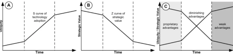
Generally, the adoption of information technology (IT) can be described by means of an S curve (cf. Fig. 1A) [10, 11, 62]. When new IT emerges at the market, it is unproven, expensive and difficult to use. Standards have not been established yet and best practices still have to established. At this point, only ”first movers” start projects based on the emerging IT. They assume that the high costs and risks for being an innovator will be later compensated by gaining competitive advantage [7].
Picking up an emerging IT at a later stage, by contrast, allows to wait until it becomes more mature and standardized, resulting in lower introduction costs and risks. However, once the value of IT has become clear, both vendors and users rush to invest in it. Consequently, technical standards emerge and license costs decrease.
Soon, the IT is widely spread, with only few enterprises having not made respective investment decisions. The S curve is then complete. Factors that typically push a new IT up the S curve include standardization, price deflation, best practice diffu-
sion, and consolidation of the vendor base. All these factors also erode the ability of IT as enabler for differentiation and competitive advantage. In fact, when dissemi- nation of IT increases, its strategic potential shrinks at the same time. Finally, once the IT has become part of the general infrastructure, it is difficult to achieve further strategic benefits (though rapid technological innovation often continues). This can be illustrated by a Z curve (cf. Fig. 1B).
Time
Ubiquity / Strategic Value
proprietary advantages
diminishing advantages
weak advantages
Time
Ubiquity
S curve of technology adoption
Time Strategic Value Z curve of
strategic value
A B C
Fig. 1 The Curves of Technology Adoption.
Considering the different curves of IT adoption, decisions about IT investments (and the right point in time to realize them) constitute a difficult task [5, 18] (cf. Fig. 1C).
Respective decisions are influenced by numerous factors [30, 36, 39, 37]. Hence, policy makers often demand for a business case [51] summarizing the key param- eters of an IT investment. Thereby, different evaluation dimensions are taken into account [31]. As examples consider the costs of an investment, its assumed profit, its impact on work performance, business process performance, and the achievement of enterprise goals.
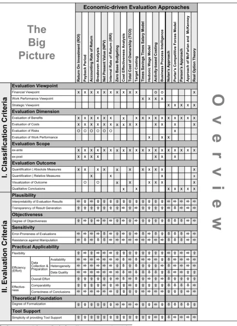
To cope with different evaluation goals, numerous evaluation approaches have been introduced (e.g. [48, 57, 58]). Fig. 2 shows results of an evaluation of 19 IT- evaluation approaches we presented in [45]. Today’s policy makers usually rely on simple and static decision models as well as on intuition and experiences rather than on a profound analysis of an IT investment decision. Further, rules of thumb such as ”invest to keep up with the technology” or ”invest if the competitors have been successful” are often applied. In many cases, there is an asymmetric consideration of costs and benefits. For example, many financial calculations (cf. Section 4) over- estimate benefits in the first years in order to realize a positive ROI. Besides, many standard evaluation approaches are often not suitable to be used at early planning stages of IT investments. In fact, many projects (especially those utilizing innovative information technology) - despite their potential strategic importance - have a nega- tive economic valuation result at an early stage. This situation results in a high risk of false rejection. This means that enterprises with independently operating busi- ness units, targeting at maximizing the equity of a company in short term, have to overcome the problem to not routinely reject truly important IT investments due to the use of insufficient evaluation techniques.
Visualization of Outcome Quantification | Absolute Measures Quantification | Relative Measures
Qualitative Conclusions
Evaluation Outcome
Interpretability of Evaluation Results Transparency of Result Generation
Error-Proneness of Evaluations Resistance against Manipulation
Flexibility
Efficiency (Effort)
DataCollection &
Preparation
Overall Effort Effective-
ness
Comparability Correctness of Conclusions
Simplicity of providing Tool Support Degree of Objectiveness
Heterogeneity Availability
Data Quality
Plausibility
Objectiveness Sensitivity
Practical Applicability
Tool Support
I. Classification Criteria
Degree of Formalization
Theoretical Foundation
Work Performance Viewpoint Financial Viewpoint
Evaluation Viewpoint
Strategic Viewpoint
Evaluation of Risks Evaluation of Benefits Evaluation of Costs
Evaluation of Work Performance
ex-post ex-ante
Evaluation Scope Evaluation Dimension
II. Evaluation Criteria Approach of McFarlan and McKenney
x x x
x
Parson’s Approach
x x x
x
Porter’s Competitive Forces Model
x x x x x
x x
Nolan’s Approach
x x x
x x
Times Savings Times Salary Model
x x
x
x
Total Cost of Ownership (TCO)
x x x
x
x
Target Costing
x x
x x
x
Internal Rate of Return (IRR)
x x
x O x
x
Net Present Value (NPV)
x x
x O x
x
Payback Period
x O x O x
x x
Return On Investment (ROI)
x x
x O x
x x
Accounting Rate of Return
x
O x x
x x
x
Zero Base Budgeting
x x x
x
x
Hedonic Wage Model
x x x
x x x
Breakeven Analysis
x
x x O
Cost Effectiveness Analysis
x x
x x
x
Activity-based Costing
o x
x x
x x
Business Process Intelligence
x o x
x x x
x x x x x x
Real Option Theory
x x
x x x x x
x
O x x x
x
Caption: x: supported o: optional :positive :negative :neutral
Economic-driven Evaluation Approaches
The Big Picture
O v e r v i e w
x
Fig. 2 IT Evaluation Approaches: The Big Picture.
1.3 Chapter Overview
Section 2 summarizes the EcoPOST cost analysis method. Section 3 introduces eval- uation patterns as an important means to simplify the application of the EcoPOST cost analysis approach. Section 4 introduces rules for designing EcoPOST eval- uation models, while Section 5 describes general modeling guidelines. Section 6 introduces a case study to illustrate the use of EcoPOST and its practical benefits.
Finally, Sections 7 and 8 conclude with a discussion of our approach and a summary.
2 The EcoPOST Cost Analysis Methodology
Our EcoPOST methodology was designed to support the introduction of Process- aware Information Systems (PAISs) [14, 50, 49] and BPM technology [13, 22, 70, 55] in the automotive industry (and was, consequently, also validated and piloted in several BPM projects in this domain). The EcoPOST methodology comprises seven steps (cf. Fig. 3). Step 1 concerns the comprehension of an evaluation scenario. This is crucial for developing problem-specific evaluation models. The following two steps (Steps 2 and 3) deal with the identification of two different kinds of Cost Fac- tors representing costs that can be quantified in terms of money (cf. Table 1): Static Cost Factors (SCFs) and Dynamic Cost Factors (DCFs).
Description
SCF Static Cost Factors (SCFs) represent costs whose values do not change during an BPM project (except for their time value, which is not further considered in the following). Typical examples: software license costs, hardware costs and costs for external consultants.
DCF Dynamic Cost Factors (DCFs), in turn, represent costs that are determined by activities related to an BPM project. The (re)design of business processes prior to the introduction of PAIS, for example, constitutes such an activity. As another example consider the performance of interview-based process analysis. These activi- ties cause measurable efforts which, in turn, vary due to the influence of intangible impact factors. The DCF
”Costs for Business Process Redesign” may be influenced, for instance, by an intangible factor ”Willingness of Staff Members to Support Process (Re)Design Activities”. Obviously, if staff members do not contribute to a (re)design project by providing needed information (e.g., about process details), any redesign effort will be inef- fective and result in increasing (re)design costs. If staff willingness is additionally varying during the (re)design activity (e.g., due to a changing communication policy), the DCF will be subject to even more complex effects.
In the EcoPOST framework, intangible factors like the one described are represented by impact factors.
Table 1 Cost Factors.
Step 4 deals with the identification of Impact Factors (ImFs), i.e., intangible fac- tors that influence DCFs and other ImFs. We distinguish between organizational, project-specific and technological ImFs. ImFs cause the value of DCFs (and other ImFs) to change, making their evaluation a difficult task to accomplish. As examples consider factors such as ”End User Fears”, ”Availability of Process Knowledge” and
”Ability to (Re-)design Business Processes”. Finally, ImFs can be static or dynamic (cf. Table 2).
Description
Static ImF Static ImFs do not change, i.e., they are assumed to be constant during an BPM project; e.g., when there is a fixed degree of user fears, process complexity, or work profile change.
Dynamic ImF
Dynamic ImFs may change during an BPM project, e.g., due to interference with other ImFs. As exam- ples consider process and domain knowledge which is typically varying during an BPM project (or a subsidiary activity).
Table 2 Impact Factors.
Unlike SCFs and DCFs the values of ImFs are not quantified in monetary terms.
Instead, they are ”quantified” by experts1using qualitative scales describing the de- gree of an ImF. As known from software cost estimation models, such as COCOMO [4], the qualitative scales we use comprise different ”values” (typically ranging from
”very low” to ”very high”). These values are used to express the strength of an ImF on a given cost factor (just like in COCOMO).
Impact Factors (ImF) Dynamic Cost Factors (DCF)
Static Cost Factors (SCF)
Steps 2 - 4 Step 5 Step 6
Design of Evaluation Models
Step 1 Step 7
Deriving Conclusions Simulation of
Evaluation Models Evaluation Context
Fig. 3 Main Steps of the EcoPOST Methodology.
Generally, dynamic evaluation factors (i.e., DCFs and dynamic ImFs) are difficult to comprehend. In particular, intangible ImFs (i.e., their appearance and impact in BPM projects) are not easy to follow. When evaluating the costs of BPM projects, therefore, DCFs and dynamic ImFs constitute a major source of misinterpretation and ambiguity. To better understand and to investigate the dynamic behavior of DCFs and dynamic ImFs, we introduce the notion of evaluation models as basic pil- lar of the EcoPOST methodology (Step 5; cf. Section 3). These evaluation models can be simulated (Step 6) to gain insights into the dynamic behavior (i.e., evolution) of DCFs and dynamic ImFs (Step 7). This is important to effectively control the design and implementation of PAIS as well as the costs of respective BPM projects.
2.1 Evaluation Models
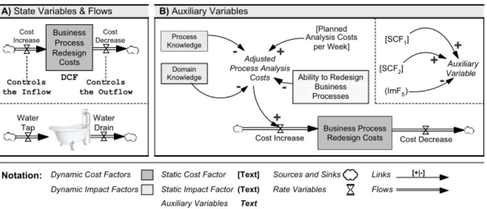
In EcoPOST, dynamic cost/impact factors are captured and analyzed by evaluation models which are specified using the System Dynamics [54] notation (cf. Fig. 4).
An evaluation model comprises SCFs, DCFs and ImFs corresponding to model vari- ables.
Different types of variables exist. State variables can be used to represent dynamic factors, i.e., to capture changing values of DCFs (e.g., the ”Business Process Re-
1The efforts of these experts for making that quantification is not explicitly taken into account in EcoPOST, though this effort also increases information system development costs.
design Costs”; cf. Fig. 4A) and dynamic ImFs (e.g., ”Process Knowledge”). A state variable is graphically denoted as rectangle (cf. Fig. 4A), and its value at time t is determined by the accumulated changes of this variable from starting point t0 to present moment t (t>t0); similar to a bathtub which accumulates – at a defined mo- ment t – the amount of water poured into it in the past. Typically, state variables are connected to at least one source or sink which are graphically denoted as cloud-like symbols (except for state variables connected to other ones) (cf. Fig. 4A). Values of state variables change through inflows and outflows. Graphically, both flow types are depicted by twin-arrows which either point to (in the case of an inflow) or out of (in the case of an outflow) the state variable (cf. Fig. 4A). Picking up again the bath- tub image, an inflow is a pipe that adds water to the bathtub, i.e., inflows increase the value of state variables. An outflow, by contrast, is a pipe that purges water from the bathtub, i.e., outflows decrease the value of state variables. The DCF ”Business Pro- cess Redesign Costs” shown in Fig. 4A, for example, increases through its inflow (”Cost Increase”) and decreases through its outflow (”Cost Decrease”). Returning to the bathtub image, we further need ”water taps” to control the amount of wa- ter flowing into the bathtub, and ”drains” to specify the amount of water flowing out. For this purpose, a rate variable is assigned to each flow (graphically depicted by a valve; cf. Fig. 4A). In particular, a rate variable controls the inflow/outflow it is assigned to based on those SCFs, DCFs and ImFs which influence it. It can be considered as an interface which is able to merge SCFs, DCFs and ImFs.
A) State Variables & Flows
Costs Business
Process Redesign
Controls the Inflow
Controls the Outflow DCF
Cost Increase
Cost Decrease
Auxiliary Variables
Rate Variables
Dynamic Cost Factors Sources and Sinks
Dynamic Impact Factors
Text Static Cost Factor [Text]
Static Impact Factor(Text) B) Auxiliary Variables
Cost Increase Cost Decrease
Adjusted Process Analysis
Costs
- -
+
Analysis Costs per Week]
+
Water Tap
Water Drain
[SCF1]
[SCF2] (ImFS)
Auxiliary Variable
+ + - -
Business Process Redesign Costs Ability to Redesign
Business Processes [Planned
Notation:
Flows Links [+|-]
Process Knowledge
Domain Knowledge
Fig. 4 Evaluation Model Notation and initial Examples.
Besides state variables, evaluation models may comprise constants and auxiliary variables. Constants are used to represent static evaluation factors, i.e., SCFs and static ImFs. Auxiliary variables, in turn, represent intermediate variables and typi- cally bring together – like rate variables – cost and impact factors, i.e., they merge SCFs, DCFs and ImFs. As example consider the auxiliary variable ”Adjusted Pro- cess Analysis Costs” in Fig. 4B, which merges the three dynamic ImFs ”Process Knowledge”, ”Domain Knowledge”, and ”Ability to Redesign Business Processes”
and the SCF ”Planned Analysis Costs per Week”. Both constants and auxiliary vari- ables are integrated into an evaluation model with links (not flows), i.e., labeled
arrows. A positive link (labeled with ”+”) between x and y (with y as dependent variable) indicates that y will tend in the same direction if a change occurs in x. A negative link (labeled with ”-”) expresses that the dependent variable y will tend in the opposite direction if the value of x changes. Altogether, we define:
Definition 2.1 (Evaluation Model) A graph EM = (V, F, L) is denotes as evaluation model, if the following holds:
• V :=S ˙∪X ˙∪R ˙∪C ˙∪A is a set of model variables with – S is a set of state variables,
– X is a set of sources and sinks, – R is a set of rate variables, – C is a set of constants,
– A is a set of auxiliary variables,
• F⊆((S×S)∪(S×X)∪(X×S))is a set of edges representing flows,
• L⊆((S×A×Lab)∪(S×R×Lab)∪(A×A×Lab)∪(A×R×Lab)∪ (C×A×Lab)∪(C×R×Lab))is a set of edges representing links with Lab :={+,−}being the set of link labels:
– (qi,qj,+)∈L with qi∈(S ˙∪A ˙∪C)and qj∈(A ˙∪R)denotes a positive link, – (qi,qj,−)∈L with qi∈(S ˙∪A ˙∪C)and qj∈(A ˙∪R)denotes a negative link.
Generally, the evolution of DCFs and dynamic ImFs is difficult to comprehend.
Thus, EcoPOST additionally provides a simulation component for capturing and analyzing this evolution (cf. Step 6 in Fig. 3).
2.2 Understanding Model Dynamics through Simulation
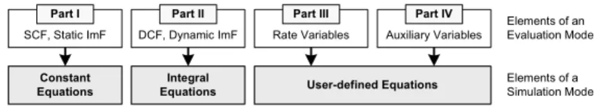
To enable simulation of an evaluation model we need to formally specify its behav- ior. EcoPOST accomplishes this by means of a simulation model based on mathe- matical equations. Thereby, the behavior of each model variable is specified by one equation (cf. Fig. 5), which describes how a variable is changing over time during simulation.
Constant Equations
Integral
Equations User-defined Equations SCF, Static ImF DCF, Dynamic ImF Rate Variables Auxiliary Variables
Elements of an Evaluation Model
Elements of a Simulation Model
Part I Part II Part III Part IV
Fig. 5 Elements of a Simulation Model.
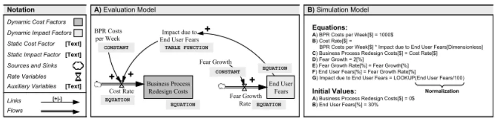
Fig. 6A shows a simple evaluation model.2Assume that the evolution of the DCF
”Business Process Redesign Costs” (triggered by the dynamic ImF ”End User Fears”) shall be analyzed. End user fears can lead to emotional resistance of users and, in turn, to a lack of user support when redesigning business processes (e.g., during an interview-based process analysis). For model variables representing an SCF or static ImF the equation specifies a constant value for the model variable;
i.e., SCFs and static ImFs are specified by single numerical values in constant equa- tions. As example consider EQUATIONA in Fig. 6B. For model variables repre- senting DCFs, dynamic ImFs or rate/auxiliary variables, the corresponding equa- tion describes how the value of the model variable evolves over time (i.e., during simulation). Thereby, the evolution of DCFs and dynamic ImFs is characterized by integral equations [16]. This allows us to capture the accumulation of DCFs and dynamic ImFs from the start of a simulation run (t0) to its end (t):
Definition 2.2 (Integral Equation) Let EM be an evaluation model (cf. Definition 2.1) and S be the set of all DCFs and dynamic ImFs defined by EM. An integral equation for a dynamic factor v∈S is defined as follows:
v(t) =tt0[in f low(s)−out f low(s)]ds+v(t0)where
• t0denotes the starting time of the simulation run,
• t represents the end time of the simulation run,
• v(t0)represents the value of v at t0,
• in f low(s)represents the value of the inflow at any time s between t0and t,
• out f low(s)represents the value of the outflow at any time s between t0and t.
A) Evaluation Model Notation
Flows Auxiliary Variables Rate Variables Dynamic Cost Factors
Links Sources and Sinks Dynamic Impact Factors
[Text]
[+|-]
Static Cost Factor [Text]
Static Impact Factor[Text]
TABLE FUNCTION
EQUATION Business Process
Redesign Costs End User
Fears Fear Growth
Rate Cost Rate
Impact due to End User Fears BPR Costs
per Week
Fear Growth
B) Simulation Model Equations:
A) BPR Costs per Week[$] = 1000$
B) Cost Rate[$] =
BPR Costs per Week[$] * Impact due to End User Fears[Dimensionless]
C) Business Process Redesign Costs[$] = Cost Rate[$]
D) Fear Growth = 2[%]
E) Fear Growth Rate[%] = Fear Growth[%]
F) End User Fears[%] = Fear Growth Rate[%]
G) Impact due to End User Fears = LOOKUP(End User Fears/100) Initial Values:
A) Business Process Redesign Costs[$] = 0$
B) End User Fears[%] = 30%
CONSTANT
CONSTANT EQUATION
EQUATION EQUATION
Normalization
+ + +
+
Fig. 6 Dealing with the Impact of End User Fears.
As example consider EQUATIONC in Fig. 6B which specifies the increase of the DCF ”Business Process Redesign Costs” (based on only one inflow). Note that in Fig. 6B the equations of the DCF ”Business Process Redesign Costs” and the dy- namic ImF ”End User Fears” are presented in the way they are specified in Vensim [65], the simulation tool used by EcoPOST, and not as real integral equations.
Rate and auxiliary variables are both specified in the same way, i.e., as user-defined functions defined over the variables preceding them in the evaluation model. In
2It is the basic goal of this toy example to illustrate how evaluation models are simulated. Generally, evaluation models are much more complex. Due to lack of space we do not provide a more extensive example here.
other words, rate as well as auxiliary variables are used to merge static and dy- namic cost/impact factors. During simulation, values of rate and auxiliary variables are dynamic, i.e., they change along the course of time. Reason is that they are not only influenced by SCFs and static ImFs, but also by evolving DCFs and dynamic ImFs. The behavior of rate and auxiliary variables is specified in the same way:
Definition 2.3 (User-defined Equation) Let EM be an evaluation model (cf. Def.
2.1) and X be the set of rate/auxiliary variables defined by EM. An equation for v∈X is a user-defined function f(v1,...,vn)with v1,...,vnbeing the predecessors of v in EM.
As example consider EQUATIONB in Fig. 6B. The equation for rate variable ”Cost Rate” merges the SCF ”BPR Costs per Week” with the auxiliary variable ”Impact due to End User Fears”. Assuming that activities for business process redesign are scheduled for 32 weeks, Fig. 7A shows the values of all dynamic evaluation factors of the evaluation model over time when performing a simulation. Fig. 7B shows the outcome of the simulation. As can be seen there is a significant negative impact of end user fears on the costs of business process redesign.
A) Computing a Simulation Run
TIME Change ($) BPR Costs ($)
00 - 0
01 1000 1000
02 1010 2010
03 1020 3030
04 1030 4060
05 1040 5100
06 1050 6150
... ... ...
30 1840 38300
31 1900 40200
32 2020 42220
Business Process Redesign Costs 60,000
45,000 30,000 15,000
0
0 2 4 6 8 10 12 14 16 18 20 22 24 26 28 30 32 Time (Weeks)
Business Process Redesign Costs : without User Fears Cost Rate ($)
1000 1010 1020 1030 1040 1050 1060 ...
1900 2020 2140
Change (%) - 2 2 2 2 2 2 ...
2 2 2
User Fears (%) 30 32 34 36 38 40 42 ...
90 92 94
B) Graphical Diagramm illustrating Simulation Outcome
Business Process Redesign Costs : with User Fears Costs
Fig. 7 Dealing with the Impact of End User Fears.
2.3 Sensitivity Analysis and Reuse of Evaluation Information
Generally, results of a simulation enable PAIS engineers to gain insights into causal dependencies between organizational, technological and project-specific factors.
This helps them to better understand resulting effects and to develop a concrete
”feeling” for the dynamic implications of EcoPOST evaluation models. To inves- tigate how a given evaluation model ”works” and what might change its behavior, we simulate the dynamic implications described by it – a task which is typically too complex for the human mind. In particular, we conduct ”behavioral experiments”
based on series of simulation runs. During these simulation runs selected simulation parameters are manipulated in a controlled manner to systematically investigate the effects of these manipulations, i.e., to investigate how the output of a simulation will
vary if its initial condition is changed. This procedure is also known as sensitivity analysis. Simulation outcomes can be further analyzed using graphical charts.
Designing evaluation models can be a complicated and time-consuming task.
Evaluation models can become complex due to the high number of potential cost and impact factors as well as the many causal dependencies that exist between them.
Taking the approach described so far, each evaluation and simulation model has to be designed from scratch. Besides additional efforts, this results in an exclusion of existing modeling experience and prevents the reuse of both evaluation and simu- lation models. In response to this problem, Section 3 introduces a set of reusable evaluation patterns (EP). EPs do not only ease the design and simulation of evalu- ation models, but also enable the reuse of evaluation information. This is crucial to foster the practical applicability of the EcoPOST framework.
2.4 Other Approaches
To enable cost evaluation of BPM technology, numerous evaluation approaches ex- ist – the most relevant ones are depicted in Fig. 2. All these approaches can be used in the context of BPM projects. However, only few of them address the specific challenges tackled by EcoPOST.
Activity-based costing (ABC) belongs to this category. It does not constitute an approach to unfold the dynamic effects triggered by causal dependencies in BPM projects. Instead, ABC provides a method for allocating costs to products and ser- vices. ABC helps to identify areas of high overhead costs per unit and therewith to find ways to reduce costs. Doing so, the scope of the business activities to be analyzed has to be identified in a first step (e.g., based on activity decomposition).
Identified activities are then classified. Typically, one distinguishes between value adding or non-value adding activities, between primary or secondary activities, and between required or non-required activities. An activity will be considered as value- adding (compared to a non-value adding one) if its output is directly related to cus- tomer requirements, services or products (as opposed to administrative or logistical outcomes). Primary activities directly support the goals of an organization, whereas secondary activities support primary ones. Required (unlike non-required) activities are those that must always be performed. For each activity creating the products or services of an organization, costs are gathered. These costs can be determined based on salaries and expenditures for research, machinery, or office furniture. Afterwards, activities and costs are combined and the total input cost for each activity is derived.
This allows for calculating the total costs consumed by an activity. However, at this stage, only costs are calculated. It is not yet determined where the costs originate from. Following this, the ”activity unit cost” is calculated. Though activities may have multiple outputs, one output is identified as the primary one. The ”activity unit cost” is calculated by dividing the total input cost (including assigned costs from secondary activities) by the primary activity output. Note that the primary output
must be measurable and its volume or quantity be obtainable. From this, a ”bill of activities” is derived which contains a set of activities and the amount of costs con- sumed by each activity. Then, the amount of each consumed activity is extended by the activity unit cost and is added up as a total cost for the bill of activity. Finally, the calculated activity unit costs and bills of activity are used for identifying candi- dates for business process improvement. In total, ABC is an approach to make costs related to business activities (e.g., business process steps) transparent. Therefore, aplying the method can be an accompanying step of EcoPOST in order to make certain cost and impact factors transparent. However, the correct accomplishment of an ABC analysis causes significant efforts and requires a lot of experience. Of- ten, it may be not transparent, for example, which costs are caused by which activity.
Besides, there are formalisms (no full evaluation approaches!) that can be applied to unfold the dynamic effects triggered by causal dependencies in BPM projects.
Causal Bayesian Networks (BN) [23], for example, promise to be a useful ap- proach. BN deal with (un)certainty and focus on determining probabilities of events.
A BN is a directed acyclic graph which represents interdependencies embodied in a given joint probability distribution over a set of variables. This allows to investigate the interplay of the components of a system and the effects resulting from this. BN do not allow to model feedback loops since cycles in BN would allow infinite feed- backs and oscillations that prevent stable parameters of the probability distribution.
Agent-based modeling provides another interesting approach. Resulting models comprise a set of reactive, intentional, or social agents encapsulating the behavior of the various variables that make up a system [6]. During simulation, the behavior of these agents is emulated according to defined rules [59]. System-level informa- tion (e.g., about intangible factors being effective in a BPM project) is thereby not further considered. However, as system-level information is an important aspect in our approach, we have not further considered the use of agent-based modeling.
Another approach is provided by fuzzy cognitive maps (FCM) [17]. An FCM is a cognitive map appyling relationships between the objects of a ”mental landscape”
(e.g., concepts, factors, or other resources) in order to compute the ”strength of impact” of these objects. To accomplish the latter task fuzzy logic is used. Most important, an FCM can be used to support different kinds of planning activities. As example consider (BPM) projects; for them, an FCM alows to analyze the mutual dependencies between respective project resources.
3 EcoPOST Evaluation Patterns
BPM projects often exhibit similarities, e.g., regarding the appearance of certain cost and impact factors. We pick up these similarities by introducing customizable patterns. This shall increase model reuse and facilitate practical use of the EcoPOST framework. Evaluation patterns (EPs) do not only ease the design and simulation of
evaluation models, but also enable the reuse of evaluation information [42, 35, 38].
This is crucial to foster practical applicability of the EcoPOST framework.
Specifically, we introduce an evaluation pattern (EP) as a predefined, but customiz- able EcoPOST model, i.e., an EP can be built based on the elements introduced in Section 2. An EP consists of an evaluation model and a corresponding simulation model. More precisely, each EP constitutes a template for a specific DCF or ImF as it typically exists in many BPM projects. Moreover, we distinguish between primary EPs (cf. Section 3.2) and secondary ones (cf. Section 3.3). A primary EP describes a DCF whereas a secondary EP represents an ImF. We denote an EP representing an ImF as secondary as it has a supporting role regarding the design of EcoPOST cost models based on primary EPs.
The decision whether to represent cost/impact factors as static or dynamic factors in EPs also depends on the model designer. Many cost and impact factors can be modeled both as static or dynamic factors. Consequently, EPs can be modeled in alternative ways. This is valid for all EPs discussed in the following.
Patterns were first introduced to describe best practices in architecture [1]. How- ever, they have also a long tradition in computer science, e.g., in the fields of software architecture (conceptual patterns), design (design patterns), and program- ming (XML schema patterns, J2EE patterns, etc.). Recently, the idea of using pat- terns has been also applied to more specific domains like workflow management [66, 68, 56, 26] or inter-organizational control [24]. Generally, patterns describe solutions to recurring problems. They aim at supporting others in learning from available solutions and allow for the application of these solutions to similar sit- uations. Often, patterns have a generative character. Generative patterns (like the ones we introduce) tell us how to create something and can be observed in the envi- ronments they helped to shape. Non-generative patterns, in turn, describe recurring phenomena without saying how to reproduce them.
Reusing System Dynamics models has been discussed before as well. Senge [61], Eberlein and Hines [15], Liehr [29], and Myrtveit [46] introduce generic struc- tures (with slightly different semantics) satisfying the capability of defining ”com- ponents”. Winch [72], in turn, proposes a more restrictive approach based on the parameterization of generic structures (without providing standardized modeling components). Our approach picks up ideas from both directions, i.e. we address both the definition of generic components and customization.
3.1 Research Methodology and Pattern Identification
As sources of our patterns (cf. Tables 3 and 4) we consider results from surveys [41], case studies [35, 43], software experiments [44], and profound experiences we gathered in BPM projects. These projects addressed a variety of typical settings in enterprise computing which allows us to generalize our experiences.
To ground our patterns on a solid basis we first create a list of candidate patterns.
For generating this initial list we conduct a detailed literature review and rely on
Pattern Name Discussed in chapter Survey Case Study Literature Experiment Experiences
Business Process Redesign Costs yes x x x - x
Process Modeling Costs yes - - x x x
Requirements Definition Costs yes - x x - x
Process Implementation Costs yes x x x x x
Process Adaptation Costs no x x x x x
Table 3 Overview of primary Evaluation Patterns and their Data Sources.
our experience with PAIS-enabling technologies, mainly in the automotive industry (e.g., [3, 34, 22]. Next we thoroughly analyze the above mentioned material to find empirical evidence for our candidate patterns. We then map the identified evalua- tion data to our candidate patterns and – if necessary – extend the list of candidate patterns.
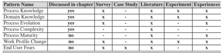
Pattern Name Discussed in chapter Survey Case Study Literature Experiment Experiences
Process Knowledge yes x - x x x
Domain Knowledge yes x - x x x
Process Evolution yes x - x - x
Process Complexity yes - - x - -
Process Maturity no - - x - x
Work Profile Change no x - x x x
End User Fears no x x x - x
Table 4 Overview of Secondary Evaluation Patterns and their Data Sources.
A pattern is defined as reusable solution to a commonly occurring problem. We re- quire each evaluation pattern to be observed at least three times in literature and our empirical research. Only those patterns, for which such empirical evidence exists, are included in the final list of patterns presented in the following.
3.2 Primary Evaluation Patterns
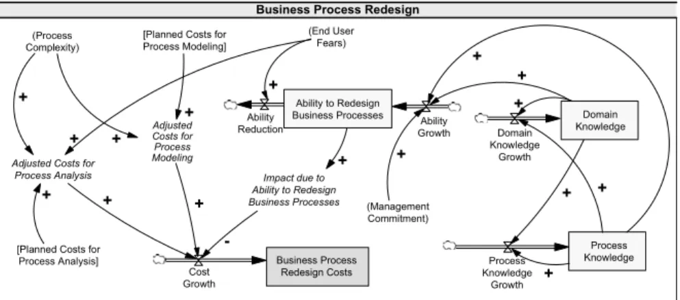
Business Process Redesign Costs. The EP shown in Fig. 8 deals with the costs of business process redesign activities. Prior to PAIS development such activities become necessary for several reasons. As examples consider the need to optimize business process performance or the goal of realizing a higher degree of process automation. This EP is based on our experiences (from several process redesign projects) that business process redesign costs are primarily determined by two SCFs:
”Planned Costs for Process Analysis” and ”Planned Costs for Process Modeling”.
While the former SCF represents planned costs for accomplishing interviews with process participants and costs for evaluating existing process documentation, the latter SCF concerns costs for transforming gathered process information into a new process design. Process redesign costs are thereby assumed to be varying, i.e., they are represented as DCF.
This EP reflects our experience that six additional ImFs are of particular importance when investigating the costs of process redesign activities: ”Process Complexity”,
Business Process Redesign
Business Process Redesign Costs Cost
Growth
Process Knowledge Ability
Growth (End User
Fears)
(Management Commitment) Adjusted Costs for
Process Analysis
Adjusted Costs for Process Modeling
+ +
Domain Knowledge
Growth
Process Knowledge
Growth
+ +
+
+
(Process Complexity)
[Planned Costs for Process Analysis]
[Planned Costs for Process Modeling]
+ +
+
+ +
+ +
Ability Reduction
Impact due to Ability to Redesign Business Processes
Ability to Redesign
Business Processes Domain
Knowledge
+
+
-
+
Fig. 8 Primary Evaluation Pattern: Business Process Redesign Costs.
”Management Commitment”, ”End User Fears”, ”Process Knowledge”, ”Domain Knowledge”, and ”Ability to Redesign Business Processes” (cf. Fig. 8). The impor- tance of these factors is confirmed by results from one of our surveys. While process analysis costs (i.e., the respective SCF) are influenced by ”Process Complexity” and
”End User Fears” (merged in the auxiliary variable ”Adjusted Costs for Process Analysis”), process modeling costs are only influenced by ”Process Complexity”
(as end users are typically not participating in the modeling process). Business pro- cess redesign costs are further influenced by a dynamic ImF ”Ability to Redesign Business Processes”, which, in turn, is influenced – according to our practical expe- riences – by four ImFs (causing the ImF ”Ability to Redesign Business Processes”
to change): ”Management Commitment”, ”End User Fears”, ”Process Knowledge”, and ”Domain Knowledge”. Note that – if desired – the effects of the latter three ImFs can be further detailed based on available secondary EPs.
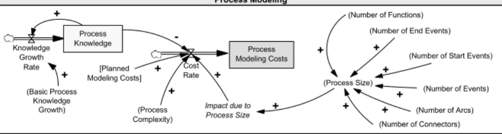
Process Modeling Costs. The EP depicted in Fig. 9 deals with the costs of process modeling activities in BPM projects. Such activities are typically accomplished to prepare the information gathered during process analysis, to assist software devel- opers in implementing the PAIS, and to serve as guideline for implementing the new process design (in the organization). Generally, there exist many notations that can be used to specify process models. Our EP, for example, assumes that process models are expressed as event-driven process chains (EPC).
Basically, this EP (cf. Fig. 9) reflects our experiences that ”Process Modeling Costs” are influenced by three ImFs: the two static ImFs ”Process Complexity” and
”Process Size” (whereas the impact of process size is specified based on a table function transforming a given process size into an EcoPOST impact rating [35]) and the dynamic ImF ”Process Knowledge” (which has been also confirmed by our survey described in [35]). The ImF ”Process Complexity” is not further discussed here. Instead, we refer to [35] where this ImF has been introduced in detail. The ImF ”Process Size”, in turn, is characterized based on (estimated) attributes of the
Process Modeling
Process Modeling Costs Cost
[Planned Rate
Modeling Costs] (Process Size)
(Process Complexity) Knowledge
Growth Rate
-
(Number of Events) (Number of Functions)
(Number of Connectors) (Number of Arcs)
+ +
+ +
(Number of Start Events) (Number of End Events)
+ +
Impact due to Process Size
+
Process Knowledge
+ +
+
+
(Basic Process Knowledge
Growth)
+
Fig. 9 Primary Evaluation Pattern: Process Modeling Costs.
process model to be developed. These attributes depend on the used modeling for- malism. As aforementioned, the EP from Fig. 9 builds on the assumption that the EPC formalism is used for process modeling. Taking this formalism, we specify process size based on the ”Number of Functions”, ”Number of Events”, ”Number of Arcs”, ”Number of Connectors”, ”Number of Start Events”, and ”Number of
”End Events”. Finally, the DCF ”Process Modeling Costs” is also influenced by the dynamic ImF ”Process Knowledge” (assuming that an increasing amount of process knowledge results in decreasing modeling costs).
Requirements Definition Costs. The EP from Fig. 10 deals with costs for defining and eliciting requirements [35]. It is based on the two DCFs ”Requirement Defini- tion Costs” and ”Requirement Test Costs” as well as on the ImF ”Requirements to be Documented”. This EP reflects the observation we made in practice that the DCF
”Requirements Definition Costs” is determined by three main cost factors: costs of a requirements management tool, process analysis costs, and requirements documen- tation costs. Costs of a requirements management tool are constant and are therefore represented as SCF. The auxiliary variable ”Adjusted Process Analysis Costs”, in turn, merges the SCF ”Planned Process Analysis Costs” with four process-related ImFs: ”Process Complexity”, ”Process Fragmentation”, ”Process Knowledge”, and
”Emotional Resistance of End Users” (whereas only process knowledge is repre- sented as dynamic ImF).
Costs for documenting requirements (represented by the auxiliary variable ”Re- quirements Documentation Costs”) are determined by the SCF ”Documentation Costs per Requirement” and by the dynamic ImF ”Requirements to be Docu- mented”. The latter ImF also influences the dynamic ImF ”Process Knowledge”
(resulting in a positive link from ”Analyzed Requirements” to the rate variable ”Pro- cess Knowledge Growth Rate”). ”Requirements Test Costs” are determined by two SCFs (”Costs for Test Tool” and ”Test Costs per Requirement”) and the dynamic ImF ”Requirements to be documented” (as only documented requirements need to be tested). Costs for a test tool and test costs per requirement are assumed to be constant (and are represented as SCFs).
Process Implementation Costs. The EP depicted in Fig. 11 deals with costs for implementing a process and their interference through impact factors [35]. An addi- tional EP (not shown here) deals with the costs caused by adapting the process(es)
Requirements Definition
Cost Rate [Planned Process
Analysis Costs]
Adjusted Process Analysis Costs
+
+
(Process Complexity) (Process Fragmentation) (Emotional Resistance
of End Users)
+ +
Process Knowledge Growth Rate
+
+
Requirements Documentation
Costs
[Costs for Requirements Management Tool]
Analyzed Requirements Completion
Rate
Documentation Rate (Basic
Comprehension Rate)
+
[Documentation Costs per Requirement]
(Relevance Rate)
Requirements Test Costs Test Cost
Rate
[Test Costs per Requirement]
[Costs for Test Tool]
Requirements to be Documented
Process Knowledge
Requirements Definition Costs
+
+ + + +
+ + +
+ +
Fig. 10 Primary Evaluation Pattern: Requirements Definition Costs.
Process Implementation
Process Implementation Costs Cost
Rate Adjusted Process
Modeling Costs [Data Modeling
Costs]
Adjusted Form Design Costs
Adjusted User/Role Management Costs
[Test Costs] [Miscellaneous Costs]
- +
+
+ + +
Domain Knowledge Growth Rate
Process Knowledge Growth Rate
+
+
(Process Complexity)
[Planned Process Modeling Costs]
[Planned User/Role Management Costs]
+
+ +
(Technical Maturity of Process Management Platform)
(Experiences in using Process Management Platform)
(Usability of Process Management Platform)
(Quality of Product Documentation) [Planned Form
Design Costs]
- + -
-
-
Process Knowledge Domain Knowledge
-
- -
Fig. 11 Primary Evaluation Pattern: Process Implementation Costs.
supported by an PAIS. This additional EP is identical to the previous EP ”Process Implementation Costs” – except for the additional ImF ”Process Evolution”.
Basic to this EP is our observation that the implementation of a process is deter- mined by six main cost factors (cf. Fig. 11): ”Adjusted Process Modeling Costs”,
”Adjusted User/Role Management Costs”, ”Adjusted Form Design Costs”, ”Data Modeling Costs”, ”Test Costs”, and ”Miscellaneous Costs”. The first three cost factors are characterized as ”adjusted” as they are influenced – according to in- terviews with software developers and process engineers – by additional process- related ImFs. Therefore, they are represented by auxiliary variables which merge the SCFs with ImFs. Process modeling costs, for example, are influenced by ”Process Knowledge”, ”Domain Knowledge”, and ”Process Complexity”. User/role manage- ment costs are only biased by ”Process Knowledge”. Form design costs are influ- enced by some technology-specific ImFs (cf. Chapter 4.7.4): ”Technical Maturity of Process Management Platform”, ”Experiences in using Process Management Plat- form”, ”Usability of Process Management Platform”, and ”Quality of Product Doc- umentation”. Note that this EP strongly simplifies the issue of process implemen- tation. In particular, we assume that the identified six main cost factors aggregate
all other potential cost factors. The SCF ”Data Modeling Costs”, for example, may include costs for providing database management functionality and for configuring a database management system. However, it is thereby not further distinguished be- tween subsidiary cost factors, i.e., other cost factors are not made explicit. If this is considered as necessary, additional SCFs or DCFs can be introduced in order to make specific cost factors more explicit. Note that we have analyzed this EP in more detail in a controlled software experiment [44].
3.3 Secondary Evaluation Patterns
We now summarize secondary EPs. Unlike a primary EP describing a particular DCF, a secondary EP represents an ImF. Again, as pattern sources we consider re- sults from two surveys [41], several case studies [35, 43], a controlled software experiment [44], and profound practical experiences gathered in BPM projects in the automotive and clinical domain [34, 28].
Process Knowledge. Fig. 12 shows an EP which specifies the ImF ”Process Knowl- edge”, i.e., causal dependencies on knowledge about the process(es) to be supported.
Process Knowledge
Process Knowledge Growth Rate +
+ AbilityRate
+
Domain Knowledge Growth Rate
+ (Emotional Resistance of End Users)
-
(Process Complexity)
(Process Fragmentation)
- + -
Domain Knowledge
Ability to Acquire Process Knowledge
Process Knowledge
Fig. 12 Secondary Evaluation Pattern: Process Knowledge.
Process knowledge includes, for example, knowledge about process participants and their roles as well as knowledge about the flow of data. Acquiring process knowl- edge necessitates the ability to acquire process knowledge. This ability, however, strongly depends on three ImFs: ”Emotional Resistance of End Users”, ”Process Complexity” and ”Process Fragmentation”. Besides, process knowledge is also in- fluenced by the dynamic ImF ”Domain Knowledge”.
Domain Knowledge. The EP from Fig. 13 deals with the evolution of domain knowledge along the course of an BPM project. Our practical experiences allow for the conclusion that ”Domain Knowledge” is a dynamic ImF influenced by three other ImFs: the period an PAIS engineer is working in a specific domain (captured by the dynamic ImF ”Experience”), the dynamic ImF ”Process Knowledge” and the complexity of the considered domain (represented by the static ImF ”Domain