Entropy–entropy dissipation techniques for nonlinear higher-order PDEs
Ansgar J¨ ungel
Vienna University of Technology, Austria Lecture Notes, June 18, 2007
1. Introduction
The goal of these lecture notes is to introduce in some aspects of entropy–entropy dis- sipation techniques. These techniques are used in order to understand the structure of nonlinear (higher-order) partial differential equations and the qualitative behavior of their solutions. In particular, we will detail a method recently developed in collaboration with Daniel Matthes (Pavia, Italy). Our approach is a more algebraic one; there exist also more geometric view points, see, for instance, the works of Carrillo, Otto, Savar´e and many others.
We have in mind the following partial differential equations:
• Porous-medium equation:
ut= ∆(um), u(·,0) =u0 ≥0 in Ω,
where Ω =Rdis the whole space or Ω =Tdis the d-dimensional torusTd∼[0, L)d, L > 0, and m > 1. The solution u(x, t) describes, for instance, the density of an unsaturated groundwater flow in a porous medium. If 0< m < 1, this equation is called the fast-diffusion equation. References: Vazquez, B´enilan/Crandell 1981.
• Thin-film equation:
ut+ div (uβ∇∆u) = 0, u(·,0) = u0 ≥0 in Ω,
whereβ >0. The solution describes, for instance, the thickness of a thin film. The case β = 1 models the flow in a Hele-Shaw cell; β = 3 models the viscous flow on a solid surface without slip driven by surface tension. References: Bertozzi, Pugh, Gr¨un, Garcke, dal Passo, Otto...
• Derrida-Lebowitz-Speer-Spohn (DLSS) equation:
ut+ div
u∇∆√
√ u u
= 0, u(·,0) =u0 ≥0 in Ω.
The solution u is the limit of a random variable related to the deviation of the interface of a two-dimensional spin system from a straight line, derived by Derrida, Lebowitz, Speer, and Spohn in 1994. It also arises in quantum semiconductor modeling. Here, u is the electron density. References: Carrillo, J¨ungel, Pinnau, Toscani, Unterreiter...
1
In order to explain what we mean by an entropy–entropy dissipation technique, we consider a simple example, the heat equation:
ut = ∆u, u(·,0) =u0 ≥0 in Td.
It is well known that for integrableu0, there exists a smooth nonnegative solution satisfying R u(x, t)dx =R
u0(x)dx =: ¯u for allt > 0. Set ¯v = ¯u/vol(Td). We introduce the following functionals which we call entropies:
E2(t) = Z
Td
(u−u)¯ 2dx, E1(t) = Z
Td
ulogu
¯ v
dx.
Observe that E1 is nonnegative. Indeed, since xlog(x/y)−x+y≥ 0 for allx, y≥ 0, we obtain
0≤ Z
Td
ulogu
¯ v
−u+ ¯v dx=
Z
Td
ulogu
¯ v
dx−
Z
Td
udx+ Z
Td
¯
vdx =E1. We claim that both functionals E1 and E2 are nonincreasing in time. First we consider E2. We obtain, using integration by parts,
dE2
dt = 2 Z
Td
(u−u)u¯ tdx= 2 Z
Td
(u−u)∆udx¯ =−2 Z
Td
|∇u|2dx≤0.
The expression on the right-hand side, R
|∇u|2dx, is called the entropy dissipation corre- sponding toE2. This term allows to conclude more than the monotonicity of E2. For this, we need the Poincar´e inequality
Z
Ω
(u−u)¯ 2dx≤CP
Z
Ω|∇u|2dx for all u∈H1(Ω).
For convex domains Ω, the constant satisfies CP ≤ (diam(Ω)/π)2 (Payne/Weinberger 1960); for Ω = T, the optimal constant is CP = (L/2π)2. The Poincar´e inequality re- lates the entropy E2 to the entropy dissipation. Then we conclude that
dE2
dt ≤ −2CP−1E2.
By Gronwall’s lemma (or just integrating the above differential inequality), E2(t)≤E2(0)e−2t/CP.
Hence, the solution u converges in the L2 norm exponentially fast to the steady state ¯u with rate 1/CP.
Next, we compute the derivative of E1: dE1
dt = Z
Td
logu
¯ v
+ 1
utdx=− Z
Td
∇
logu
¯ v
+ 1
· ∇udx=−4 Z
Td
|∇√ u|2dx.
Again, we need an expression relating the entropy E1 and the entropy dissipation. This is done by the logarithmic Sobolev inequality
Z
Ω
ulogu
¯
vdx≤CL
Z
Ω|∇√
u|2dx for all √
u∈H1(Ω), u≥0.
If Ω =T, the constantCLequals L2/2π2 (Rothaus 1980, Weissler 1980, or Dolbeault/Gen- til/J¨ungel 2006). Then we have
dE1
dt ≤ −4CL−1E1 and E1(t)≤E1(0)e−4t/CL.
The solution converges in the “entropy norm” exponentially fast to its steady state with rate 4/CL.
Sometimes, one is rather interested in the convergence of the solution in a Lebesgue norm, for instance in theL1 norm. The above estimate allows to derive such a conclusion by means of the Csisz´ar-Kullback inequality:
Z
Ω
ulogu v
−u+v
dx≥CK Z
Ω|u−v|dx2
for all u, v ∈L1(Ω), u, v ≥0.
By Bartier/Dolbeault/Illner/Kowalczyk 2006, the constant CK ≤ 1/4 max{kukL1,kvkL1}. Therefore,
ku−u¯kL1(Td) ≤ s
E1(0) CK
e−2t/CL.
The above example shows that the entropy–entropy dissipation method consists of the following ingredients:
• entropy functional,
• entropy–entropy dissipation inequality (depending on the PDE under considera- tion),
• study of the long-time behavior: relation between the entropy and entropy dissipa- tion.
In the following section we will specify which kind of entropies are of interest. An important step is the derivation of the entropy–entropy dissipation inequality, which was easy in the case of the heat equation, but which is rather involved for the (fourth-order) equations mentioned above. An algorithmic construction method will be presented in section 3.
Section 4 is concerned with additional results. We conclude in section 5 with some open problems.
2. Definitions and explanations
Let u(x, t) be a nonnegative solution to a PDE for x ∈ Ω, t > 0, and let E and P be functionals, defined byuand its derivatives. We call (E, P) an entropy–entropy production pair if and only if
(1) dE
dt +P ≤0 and E, P ≥0.
We are interested in the following entropies:
• Zeroth-order entropies:
Eα = 1 α(α−1)
Z
Ω
uαdx, α 6∈ {0,1}, E1 =
Z
Ω
(u(logu−1) + 1)dx, α= 1, E0 =
Z
Ω
(u−logu)dx, α= 0.
• First-order entropies:
E˜α = Z
Ω|∇(uα/2)|2dx, α6= 0.
Clearly, higher-order entropies can be also defined but we will study only entropies of zeroth or first order. The functional E1 represents (up to a sign) the physical entropy.
The functionalsEα give rise to estimates in the Lebesgue space Lα; ˜E2 provides a gradient estimate in L2, whereas ˜E1 is called the Fisher information.
Examples for entropy productions are, in one space dimension, P =
Z
Ω
(uα/2)2xdx, P = Z
Ω
(uα/2)2xxdx etc.
In the following we explain which kind of informations can be drawn from inequalities like (1).
1. Long-time behavior. Let u be a solution of a PDE and (E, P) be an entropy–entropy dissipation pair satisfyingdE/dt+c1P ≤0, wherec1 >0 is a constant. If there is a relation between the entropy and the entropy production of the form E ≤ c2P for some constant c2 >0 (like the Poincar´e or logarithmic Sobolev inequality; see the previous section), we derive
dE dt +c1
c2E ≤0.
Thus, by Gronwall’s lemma, E(t) ≤ E(0)e−c1t/c2 and we have an exponential decay with rate c1/c2. In some situations (for instance, whole-space problems without confinement), we can only expect to obtain inequalities like Eγ ≤ c2P for some γ > 1 (see Car- rillo/Dolbeault/Gentil/J¨ungel 2006 for some examples) such that
dE dt +c1
c2
Eγ ≤0.
Hence, after integration, E(t) behaves like t−1/(γ−1) for t → ∞. This gives an algebraic decay rate.
2. Existence of solutions. An existence proof of a nonlinear parabolic PDE of the type ut = F(u,∇u, . . .) with some initial and boundary conditions may have the following steps. First, approximate the PDE appropriately. An example is to replace the derivative ut by (u(t)−u(t− △t))/△t and to solve the sequence of elliptic problems
u(t)−(△t)F(u(t),∇u(t), . . .) = (△t)u(t− △t),
where z = u(t− △t) is given. Second, define a fixed-point operator by “linearizing” the elliptic problem, S :B →B, w7→u, for instance,
u−∆u+ (△t)F(w,∇w, . . .)−∆w
= (△t)z.
If the existence of a fixed point will be proved by the Leray-Schauder fixed-point theorem, we need appropriate uniform estimates for all fixed points. We recall the fixed-point theorem.
Leray-Schauder’s fixed-point theorem: Let B be a Banach space, S : B × [0,1] → B compact (i.e. S(B1(0)) is a compact set, where B1(0) = {x ∈ B :kxkB <1}) such thatS(x,0) = 0 for all x∈B and
∃c > 0 :∀x∈B, σ ∈[0,1], x=S(x, σ) :kxkB ≤c.
Thenx7→S(x,1) has a fixed point.
Third, let us suppose that for a given fixed point of S, i.e. a solution of the PDE under consideration (maybe including σ), we are able to prove an entropy–entropy dissipation inequality
(2) E(t) +
Z t 0
P(s)ds≤E(0).
Usually, the production term P contains derivatives (see above). The inequality should satisfy two requirements: (i) the estimate on Rt
0P ds should imply a bound for kukX in a Banach space X and (ii)X is compactly embedded inB. Then the Leray-Schauder fixed- point theorem applies. In general, the crucial step of the existence proof is the estimate (2).
3. Regularity of solutions. For instance, in the case of the DLSS equation with initial data
√u0 ∈ H1(Ω), it is possible to prove for a solution u that (see Dolbeault/Gentil/J¨ungel 2006)
Z
Ω
(√
u)2x(t)dx+c Z t
0
Z
Ω
(√
u)2xx+ (√ u)2xxx
dx≤ Z
Ω
(√u0)2xdx.
Thus, since u∈ L∞(0, T;L1(Ω)), √
u ∈L∞(0, T;H1(Ω))∩L2(0, T;H3(Ω)). This provides (slightly) more regularity than the definition of a weak solution to the DLSS equation.
4. Positivity of solutions. The proof of positivity is usually shown by means of the maximum principle. However, for higher-order equations, this principle generally does not apply, and other techniques have to be employed. The entropy–entropy dissipation inequalities can be helpful for some PDEs. The proof of positivity depends much on the studied PDE so that we present only an example, the 1D thin-film equation. Let the initial datumu0 ∈H1(0,1) be positive, 72 ≤β≤5, and let u be a solution to
ut+ (uβuxxx)x = 0 in (0,1), t >0, ux =uβuxxx = 0 for x∈ {0,1}, u(·,0) =u0 >0.
Beretta/Bertsch/dal Passo 1995 have shown that u∈C1/8([0, T];C1/2([0,1])) and that for all 32 ≤α+β ≤3,
(3)
Z 1 0
uα(x, t)dx is finite for all t >0.
(We will prove the second statement in section 3.) We claim that from this (entropy) estimate, the positivity of ufollows. The following proof is taken from Beretta et al. 1995.
Suppose, by contradiction, that there isx0 such that u(x0, t) = 0. By the regularity on u, 0≤u(x, t)≤C|x−x0|1/2 uniformly in t. Let us take α=−2 in (3). This is admissible since then 32 ≤ −2 +β ≤3 is equivalent to 72 ≤β ≤5. We obtain
∞>
Z 1 0
u(x, t)αdx≥Cα Z 1
0 |x−x0|α/2dx=C−2 Z 1
0 |x−x0|−1dx=∞, contradiction. Thus, u(x, t)>0 for all x (and t).
5. New functional inequalities. Using the entropy–entropy dissipation method, we can also prove inequalities involving derivatives of functions like
Z
T
uα(logu)4xdx≤Cα
Z
T
uα(logu)2xxdx, Cα = 9 α2. We refer to section 4 for details.
3. Entropy construction method
3.1. Idea of the method. We introduce the technique by first studying a rather simple example, the 1D thin-film equation
(4) ut+ (uβuxxx)x= 0 in T, u(·,0) =u0. Our goal is to derive estimates of the type
dEα
dt +P ≤0, where Eα is a zeroth-order entropy, Eα =R
uαdx/α(α−1). For this, we assume that u is a positive smooth solution to (4), we take the time derivative ofEα and integrate by parts once:
dEα
dt = 1 α−1
Z
T
uα−1utdx= Z
T
uα+β−2uxuxxxdx=:−Q.
In order to show that Q≥0, we integrate by parts once more:
Q= (α+β−2) Z
T
uα+β−3 u2xuxx
| {z }
=13(u3x)x
dx+ Z
T
uα+β−2u2xxdx
=−1
3(α+β−2)(α+β−3) Z
T
uα+β−4u4xdx+ Z
T
uα+β−2u2xxdx.
(5)
Now, Q≥0 if (α+β−2)(α+β−3)≤0 or if 2≤α+β ≤3.
Although the above computation shows the claim, there are two disadvantages of this approach:
• One may wonder if the second term (5) can compensate the first term in case the factor (α+β−2)(α+β−3) is negative. This is indeed the case. We will show below that Q ≥ 0 if (and only if) 32 ≤ α+β ≤ 3. Thus, the parameter range
3
2 ≤α+β <2 is not covered by the above computation.
• The integration by parts have been done in a non-systematic and ad-hoc way. Better results can be obtained by a different integration by parts (see below). Moreover, in several space dimensions, there are many possible integration by parts, and it is not clear how to apply them.
In view of these drawbacks, we suggest an approach which is based on a systematic use of integration by parts. For this, we describe integration by parts in a different way. The computation
(6) Q=− Z
T
uα+β−2uxuxxxdx = (α+β−2) Z
T
uα+β−3u2xuxxdx+ Z
T
uα+β−2u2xxdx can be written in the form
I2 = Z
T
uα+β
(α+β−2)ux u
2uxx
u +uxx u
2
+ux u
uxxx u
dx=
Z
T
uα+βux u
uxx u
xdx = 0.
Then (6) corresponds to
Q=Q+c·I2 with c= 1.
How many integration-by-parts rules do exist? There are three rules. The other two read as
I1 = Z
T
uα+β
(α+β−3)ux u
4
+ 3ux u
2uxx u
dx=
Z
T
uα+βux u
3
xdx= 0, I3 =
Z
T
uα+β
(α+β−1)ux
u uxxx
x + uxxxx
u
dx= Z
T
uα+βuxxx
u
xdx= 0.
The number of rules is determined by all integersp1,p2, andp3such that 1·p1+2·p2+3·p3 = 3. Thus,
(p1, p2, p3) = (3,0,0),(1,1,0),(0,0,1),
and there are exactly three rules. Then we can reformulate the problem of proving Q≥0 as
∃c1, c2, c3 ∈R:Q=Q+c1I1+c2I2+c3I3 ≥0.
Clearly, sinceIk = 0 for k = 1,2,3, the above equality is trivial.
Now comes our main idea. We identify the integrands (up to the factor uα+β) as poly- nomials via the identificationξ1 , uux, ξ2 , uuxx etc. Therefore, with ξ= (ξ1, ξ2, ξ3),
Q corresponds toS(ξ) =−ξ1ξ3,
I1 corresponds to T1(ξ) = (α+β−3)ξ14+ 3ξ12ξ2, I2 corresponds to T2(ξ) = (α+β−2)ξ12ξ2+ξ22+ξ1ξ3, I3 corresponds to T3(ξ) = (α+β−1)ξ1ξ3+ξ4.
The polynomialsTk are termed shift polynomials. If we can solve the polynomial problem (7) ∃c1, c2, c3 ∈R:∀ξ ∈R3 : (S+c1T1+c2T2+c3T3)(ξ)≥0,
then we have a pointwise estimate for the integrands, andQ≥0 follows.
Remark 1. We show a much stronger estimate than justQ=R
uα+βf(u, ux, uxx, . . .)dx ≥ 0 since we try to prove that f(u, ux, uxx, . . .)≥0 for allx∈T. One may wonder if by this approach entropy estimates may get lost. It is possible to show (see J¨ungel/Matthes 2006) that this is not the case for the 1D thin-film and DLSS equation. It is not known if this is true for the multi-dimensional situation or more general equations.
If the problem (7) is solved, we have only shown that the entropy is nonincreasing in time. In order to prove the stronger resultdE/dt+cP ≥0, where c >0 is a constant and P a (nonnegative) entropy production, we can proceed in a similar way as above. Since Q=−dE/dt, we have to prove that there exists a constant c >0 such that −Q+cP ≥0 or, with the above integration-by-parts rules,
(8) ∃c1, c2, c3 ∈R, c >0 :−Q+cP +c1I1+c2I2+c3I3 ≥0.
This problem is of the same type like (6) and therefore, it can be “translated” to a polyno- mial problem similar to (7). Possible entropy productions, for this fourth-order equation, are, for instance,
P = Z
T
(u(α+β)/4)4xdx, P = Z
T
(u(α+β)/2)2xxdx, P = Z
T
uα+β−2u2xxdx.
We summarize our algorithm:
(1) Calculate the functional Q and “translate” it into a polynomial S. (This step depends on the equation at hand.)
(2) Determine the shift polynomialsTk which represent the integration-by-parts rules.
(This step only depends on the order of the equation but not on the structure of the equation except for the parameter β.)
(3) Decide for which parameters α the problem (7) can be solved. This shows that Eα
is nonincreasing in time.
(4) Decide for which parameters α the problem (8) can be solved. As a result, the entropy–entropy production inequalitydEα/dt+cP ≤0 holds.
It remains to solve the problem (7). This is a decision problem which is well-know in real algebraic geometry. It was shown by Tarski in 1951 that such problems can be always treated in the following sense:
A quantified statement about polynomials can be reduced to a quantifier- free statement about polynomials in an algorithmic way.
Solution algorithms for the above quantifier elimination problem have been implemented, for instance, in Mathematica. There are also tools specialized on quantifier elimination, like QEPCAD (Quantifier Elimination using Partial Cylindrical Algebraic Decomposition), see Collins/Hong 1991. The advantage of these algorithms is that the solution is complete and exact. The disadvantage is that the complexity of the algorithms is doubly exponential in the number of variablesξiandci. An alternative approach is given by the sum-of-squares (SOS) method. This method tries to write the polynomial as a sum of squares. Therefore, the answer may be not complete since there are polynomials which are nonnegative but which cannot be written as a sum of squares. Fortunately, for some decision problems arising from 1D fourth-order equations, we can solve the problems directly without going into real algebraic geometry. This will be explained below.
We notice that our method is formal in the sense that positive smooth solutions have to be assumed in order to justify the calculations. The proofs can be made rigorous if an appropriate approximation of the original equation is available which (i) allows for positive smooth solutions and (ii) does not destroy the entropic structure. Clearly, such an approximation depends much on the specific equation.
3.2. The general scheme. In the following we only present the general scheme for spatial one-dimensional equations. A systematic treatment of multi-dimensional problems is in progress (but see section 4). We are concerned with equations of the type
ut=
uβ+1qux
u ,u2xx
u , . . . , ux...x
x
x inT, t >0,
where the derivativesux...x are up to order k−1 (with even k) andq(ξ1, . . . , ξk−1) is a real polynomial,
q(ξ1, . . . , ξk−1) = X
p1,...,pk−1
cp1,...,pk−1ξ1p1· · ·ξkpk−1
such that at most those coefficients cp1,...,pk−1 ∈Rwith 1·p1+· · ·+ (k−1)·pk−1 =k−1 are nonzero. We denote the set of those polynomials as Σk−1. In this notation, q ∈Σk−1. An example is the thin-film equation with k = 4 and q(ξ) = ξ3. In order to distinguish between the polynomial q and its differential operator, we set
Dq(u) =qux
u ,u2xx
u , . . . ,ux...x
x . Letu be a positive smooth solution to
ut= (uβ+1Dq(u))x, u(·,0) = u0,
where q ∈ Σk−1, with periodic boundary conditions. We need some definitions. For this, lets(u) be one of the following functions:
s(u) = uα
α(α−1), s(u) = u(logu−1) + 1, s(u) =u−logu,
where α∈R, α6∈ {0,1}. Notice that s′′(u) =uα−1.
• The functionE(t) =R
s(u(x, t))dx is called an entropyif E(t) is nonincreasing.
• The function P(t) = R
uα+βDp(u)dx with p ∈ Σk is called an entropy production for the entropy E if there exists c >0 such that for all t >0,
dE
dt +cP ≤0.
• The entropy E is calledgeneric if P is an entropy production for all p∈Σk. Step 1: characteristic polynomials. Taking the derivative of a function E and integrating by parts gives
dE dt =
Z
T
s′(u)utdx=− Z
T
s′′(u)ux(uβ+1Dq(u))dx=− Z
T
uα+βux
uDq(u)dx.
For the entropy–entropy dissipation method, we need to modify the polynomial corre- sponding to (ux/u)Dq(u). Therefore, we call s0 ∈Σk a characteristic polynomial if
dE dt =−
Z
T
uα+βDs0(u)dx.
Clearly, there is at least one characteristic polynomial, namely s0(ξ) = ξ1q(ξ1, . . . , ξk−1), which is called a canonical (characteristic) polynomial.
Step 2: shift polynomials. The integration-by-parts rules can be formalized as follows. We introduce for γ ∈R the operator δγ : Σk−1 →Σk by
(uγDp(u))x =uγDδγp(u), p∈Σk−1.
An explicit calculation shows that the image of the monomial p(ξ) = ξ1p1· · ·ξk−1pk−1 is (9) δγp(ξ) = (γ −p1− · · · −pk−1)ξ1p(ξ) +p1
ξ2
ξ1
p(ξ) +· · ·+pk−1
ξk
ξk−1
p(ξ).
Example 2. The three monomials r1(ξ) = ξ31,r2(ξ) =ξ1ξ2,r3(ξ) =ξ3 form a basis of Σ3. Then formula (9) gives
T1(ξ) := δα+βr1(ξ) = (α+β−3)ξ14+ 3ξ12ξ2, T2(ξ) := δα+βr2(ξ) = (α+β−2)ξ12ξ2+ξ22+ξ1ξ3, T3(ξ) := δα+βr3(ξ) = (α+β−1)ξ1ξ3+ξ4.
These polynomials are a basis of the linear space δα+βΣ3. They express our integration- by-parts rules.
In view of the above example, we choose a basis of monomials ri ∈ Σk−1, i = 1, . . . , d.
Then the functions Ti = δα+βri are also linearly independent. We will call them shift polynomials. We have to solve the following problem:
∃c1, . . . , cd∈R:∀ξ∈Rk :s(ξ) = (s0+c1T1+· · ·+cdTd)(ξ)≥0.
If this is true thenE is an entropy. This decision problem can be simplified by eliminating some integration-by-parts rules which are not useful. In terms of polynomial manipulations, this leads to the notion of a normal form.
Step 3: decision problems. We call a characteristic polynomialp∈Σkto be innormal form if for eachj, the highest exponent with which ξj occurs in pis even. Otherwise, ξja → −∞
if ξj → −∞ and the polynomial cannot be nonnegative.
Example 3. We are looking for the normal forms for s0+c1T1+· · ·+cdTd in the case of the thin-film equation. Recall that s0(ξ) =−ξ1ξ3. Since T3 contains ξ4 =ξ41 and 1 is odd, c3 = 0. The constant c2 must be chosen to eliminate ξ3 =ξ31. Hence, c2 = 1. There is no restriction onc1. Thus, the normal forms are given by
s :=s0+c1·T1+ 1·T2+ 0·T3 = (α+β−3)c1ξ14+ (α+β−2 + 3c1)ξ12ξ2+ξ22. Step 4: entropy production. Finally, we turn to an algebraic formulation of the entropy production P =R
uα+βDp(u)dx. To prove dE/dt+cP ≤ 0 for some c >0, it is sufficient to show that
s(ξ)−c·p(ξ)≥0.
Again, a decision problem has to be solved. Recall that an entropy E is generic if this inequality is true for all p ∈ Σk, with constants c depending on p. The idea behind this notion is that, for small c >0, s−cp is a polynomial with an c-small perturbation in the coefficients.
3.3. Solution of some decision problems. The notion of normal forms allows to reduce the number of variablesci in the decision problem. In this subsection, we give some lemmas by which decision problems for polynomials up to sixth order can be solved.
Lemma 4. Let the real polynomial p(ξ1, ξ2) = a1ξ14 +a2ξ12ξ2 +a3ξ22 be given. Then the quantified expression
∀ξ1, ξ2 ∈R: p(ξ1, ξ2)≥0 is equivalent to the quantifier-free statement that
either a3 >0 and 4a1a3−a22 ≥0 or a3 =a2 = 0 and a1 ≥0.
Lemma 5. Let the real polynomial
p(ξ1, ξ2, ξ3) = a1ξ61 +a2ξ14ξ2+a3ξ31ξ3+a4ξ12ξ22+a5ξ1ξ2ξ3+ξ32 be given. Then the quantified formula
∀ξ1, ξ2, ξ3 ∈R: p(ξ1, ξ2, ξ3)≥0 is equivalent to the quantifier free formula
either 4a4−a25 >0 and 4a1a4−a1a25−a22−a23a4+a2a3a5 ≥0 or 4a4−a25 = 2a2 −a3a5 = 0 and 4a1−a23 ≥0.
The (elementary) proofs of these lemmas can be found in J¨ungel/Matthes 2006. We can employ Lemma 4 to solve the decision problem for the 1D thin-film equation,
∃c1 ∈R:∀ξ ∈R2 : (s0+c1T1+T2)(ξ) = (α+β−3)c1ξ14+ (α+β−2 + 3c1)ξ12ξ2+ξ22 ≥0.
Since the coefficient for ξ22 is positive, the nonnegativity is guaranteed if and only if 0≤4a1a3−a22 = 4c1(α+β−3)−(α+β−2 + 3c1)2
=−9 c1+1
9(α+β)2
− 8
9(α+β)2+ 4(α+β)−4.
Choosing the maximizing valuec1 =−(α+β)/9, this inequality is satisfied if and only if 0≤ −8(α+β)2+ 36(α+β)−36.
The roots of the polynomial x 7→ −8x2 + 36x−36 are x1 = 3/2 and x2 = 3. Therefore, the inequality is valid if and only if 32 ≤α+β ≤3.
Entropy productions are derived by showing (s0 +c1T1 −cp)(ξ) ≥ 0 for some (small) c > 0. If, for instance, the entropy production is given by P = R
uα+β−2u2xxdx, we have p(ξ) = ξ22, and we need to solve
∃c1 ∈R, c >0 :∀ξ ∈R2 : (α+β−3)c1ξ14+ (α+β−2 + 3c1)ξ12ξ2+ (1−c)ξ22 ≥0.
It can be easily seen that this problem is solvable if 32 < α+β <3.
In the nongeneric cases α+β = 3/2 and α+β = 3, there may be still specific entropy productions. For instance, let α +β = 3/2. We choose c1 = −1/6 in the polynomial s0+c1T1+T2 which gives
(s0+c1T1+T2)(ξ) = 1
4ξ41 +ξ12ξ2 +ξ22 = ξ2− 1
2ξ122
. The corresponding functional reads as
(10) dEα
dt =− Z
T
u3/2uxx
u − ux
2u 2
dx =− Z
T
u1/2(u1/2)2xxdx.
Similarly, the caseα+β = 3 can be treated: Choosing c1 =−1/3 leads to
(11) dEα
dt =− Z
T
uu2xxdx.
We have shown:
Theorem 6. The functionals Eα(t) are nonincreasing in time (along solutions of the 1D thin-film equation) if 32 ≤ α+β ≤3. Moreover, if 32 < α+β <3, there exists c >0 such
that dEα
dt +c Z
T
uα+β−2u2xx+ (u(α+β)/2)2xx+ (u(α+β)/4)4x
dx≤0.
Furthermore, if α+β = 3/2 or α+β = 3, the inequalities (10), (11), respectively, hold.
More precisely, we have shown the last inequality only for the first entropy production term but the proof for the remaining terms is similar.
3.4. Second example: DLSS equation. We consider the DLSS equation ut+ (u(logu)xx)xx = 0 inT, t >0, u(·,0) =u0. Since
−(u(logu)xx)x =u
−ux
u 3
+ 2ux
u uxx
u − uxxx
u
,
we haveut= (uDp(u))xwith p(ξ) =−ξ13+ 2ξ1ξ2−ξ3. Hence, the (canonical) characteristic polynomial is s0(ξ) =ξ1p(ξ) =−ξ41 + 2ξ12ξ2 −ξ1ξ3. The shift polynomials are the same as for the thin-film equation choosing β = 0:
T1(ξ) = (α−3)ξ14+ 3ξ21ξ2, T2(ξ) = (α−2)ξ12ξ2+ξ22+ξ1ξ3, T3(ξ) = (α−1)ξ1ξ3+ξ4.
Similarly, the most general normal form is given by
s0+c·T1+ 1·T2+ 0·T3 = (c(α−3)−1)ξ14+ (3c+α)ξ12ξ2+ξ22. This polynomial is nonnegative for all ξ ∈R3 if, by Lemma 4,
0≤4a1a3−a22 = 4(c(α−3)−1)−(3c+α)2 =−9c2−2(α+ 6)c−(4 +α2)
=−9 c+1
9(α+ 6)2
− 8 9α
α−3 2
.
Choosing the maximizing valuec=−(α+ 6)/9, we obtain 0≤ −8
9α α− 3
2
,
This inequality is satisfied if and only if 0≤α ≤3/2. As before, the generic entropies are those for which 4a1a3−a22 >0, corresponding to 0< α <3/2.
Next, we turn to the nongeneric entropies α= 0 andα = 3/2. For α= 0, we have s0(ξ) +cT1(ξ) +T2(ξ) = −(3c+ 1)ξ14 + 3cξ12ξ2+ξ22.
Taking c=−2/3 gives (s0 +cT1 +T2)(ξ) = ξ41 −2ξ12ξ2+ξ22 = (ξ12−ξ2)2 which translates to the entropy production
Z
T
ux
u 2
− uxx
u 2
dx= Z
T
(logu)2xxdx.
Similarly, if α= 3/2, we takec=−5/6, leading to the entropy production 4
Z
T
u1/2(u1/2)2xxdx.
We summarize these results in the following theorem.
Theorem 7. The functionals Eα(t) are nonincreasing in time (along solutions of the 1D DLSS equation) if 0≤α≤3/2. Moreover, if 0< α <3/2, there exists c >0 such that
dEα
dt +c Z
T
uα−2u2xx+ (uα/2)2xx+ (uα/4)4x
dx≤0.
Furthermore,
dEα
dt + Z
T
(logu)2xxdx≤0 if α= 0, dEα
dt + 4 Z
T
u1/2(u1/2)2xxdx≤0 if α= 3 2. 4. Additional results
4.1. Higher-order entropies. Clearly, the approach of the previous section also applies to higher-order entropies, like the first-order entropies
E = Z
Ω
(uα/2)2xdx, α >0.
Consider again the 1D thin-film equation. Then, taking the derivative, dE
dt = 2 Z
Ω
(uα/2)x(uα/2)txdx=−2 Z
Ω
(uα/2)xx
α
2uα/2−1utdx
=−α Z
Ω
(uα/2)xxuα/2−1(uβuxxx)xdx.
Thus, we have to find all integration-by-parts rules involving a total of six derivatives. It can be seen that there are seven integration-by-parts rules giving seven shift polynomials.
Some of the shift polynomials do not need to be taken into account (i.e., the normal form does not contain them), like
T(ξ) = (α+β−1)ξ1ξ5+ξ6,
sinceξ6 appears in odd order. Writing down the normal form leads to the following decision problem:
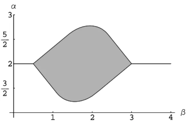
∃c1, c2 ∈R:∀ξ∈R3 : (α+β−5)c1ξ16+ (5c1+ (α+β−4)c2)ξ14ξ2+ 3c2ξ12ξ22 + (12(α2−5α+ 6)ξ13ξ3+ (2α−4)ξ1ξ2ξ3+ξ32 ≥0.
The quantifier elimination can be performed using Lemma 5 for polynomials in Σ6 in three variables up to order six. The result is displayed in Figure 1. (This result has been first found by Laugesen 2005.) Notice that there is always a trivial first-order entropy corresponding to α = 2, reading E =R
u2xdx. In fact, the corresponding entropy–entropy inequality can be easily obtained by differentiation:
d dt
Z
T
u2xdx = 2 Z
T
uxutxdx=−2 Z
T
uxxutdx = 2 Z
T
uxx(uβuxxx)xdx=−2 Z
T
uβu2xxxdx.
A similar result can be derived for the DLSS equation. The functional E =R
(uα/2)2xdx is an entropy if α lies in between the two reals roots of 20 − 100α + 53α2, i.e. α ∈ (0,2274. . . ,1.6593. . .).
The situation is more complicated concerning second-order entropies since even for fourth-order equations, polynomials of order 8 need to be solved. We have not found second-order entropies for the thin-film or DLSS equation using quantifier elimination or
1 2 3 4 Β
3 2 2
5 2 3
Α
1 2 3 4 Β
3 2 2
5 2 3
Α
Figure 1. Values ofα and β providing an entropy.
the sum-of-squares method. This does not mean that there are no second-order entropies for these equations since our proof is based on pointwise estimates of the integrand.
4.2. Multi-dimensional equations. In principle, the strategy for the one-dimensional PDEs can be generalized in a straight forward way to multi-dimensional equations. In this situation, we have to deal with polynomial variables for all the partial derivatives.
Integration-by-parts rules are obtained by differentiating products in all variables. Practi- cally, this strategy is useless since it leads to polynomial expression in many variables ξk
and a huge number of shift polynomials Ti. A better approach is not to incorporate all products of differential expressions. As this is still current research, we will only sketch some ideas.
Our main idea is to exploit the symmetry of the problem. For instance, consider the problem of deriving first-order entropies for a fourth-order equation indspace dimensions.
Then the polynomials are a linear combination of 14O(d)-invariant scalar expressions like k∇3uk3, ∇∆u· ∇2u· ∇u, |∇u|6, . . . ,
where∇2udenotes the Hessian ofuand∇3uthe corresponding 3-tensor. Then we perform the following steps:
(1) Restrict to those integration-by-parts rules which can be written in the above 14 expressions alone. This leads to 7 decision variables.
(2) Perform a rotation and/or dilation to eliminate all dependencies on first derivatives.
The remaining polynomials are at most of order three.
(3) Eliminating the third-order terms gives a quadratic problem in RN, where the variables represent derivatives of second and third order.
(4) Decomposing RN into certain subspaces, it is enough to consider the quadratic problem on the subspaces. This yields a semi-definite programming problem in 9 variables with 7 parameters.
Example 8. In this example we detail the problem of finding zeroth-order entropies for the thin-film equation,
ut+ div (uβ∇∆u) = in Td, t >0, u(·,0) =u0,
we proceed slightly different than above (see J¨ungel/Matthes 2006). There are 7 scalar expressions containing exactly four derivatives:
ηG4 =u−4|∇u|4, η2L=u−2(∆u)2, trace(ηH2) =u−2trace(∇2u)2,
ηG2ηL=u−3|∇u|2∆u, ηG2ηH =u−1(∇u)⊤∇2u(∇u), ηGηT =u−2∇∆u· ∇∆u, ηD =u−1∆2u.
The expressions on the left-hand sides have to be read as formal symbols and not as products. There are four shift polynomials of interest:
T1(η) = (α+β−3)η4G+η2GηL+ 2ηG2ηH, T2(η) = (α+β−2)η2GηL+η2L+ηGηT,
T3(η) = (α+β−2)η2GηH + trace(ηH2) +ηGηT, T4(η) = (α+β−1)ηGηT +ηD.
The (canonical) characteristic polynomial is s0(η) = −ηGηH. It can be shown that the general normal form reads as follows:
(s0+c1T1+c2T2+c3T3)(η) =c1(α+β−3)ηG4 +c2η2L+c3trace(η2H)
+ ((α+β−2)c2+c1)ηG2ηL+ ((α+β−2)c3+ 2c1)ηG2ηH, and c2 and c3 satisfy the relation c2+c3 = 1. Actually, it is even possible to reduce the quantifier elimination problem to three scalar variables kηGk, (trace(ηH2))1/2, and ηL and one decision variable. Then, employing the algebra tool QEPCAD, one can show that the zeroth-order functionals are entropies if 3/2≤α+β ≤3. This is the same condition as in the one-dimensional case.
4.3. New functional inequalities. The entropy–entropy dissipation approach can be also used to prove some functional inequalities. As an example, we will show that for all positive smooth functions u, it holds
(12)
Z
T
uα(logu)4xdx≤ 9 α2
Z
T
uα(logu)2xxdx, α >0.
This inequality resembles the logarithmic Sobolev inequality, mentioned in the introduc- tion,
Z
T
u2log u2
M2dx≤C Z
T
u2(logu)2xdx, where M2 =R
u2dx/L and T∼[0, L).
Inequality (12) can be written as 0≤
Z
T
uα (logu)2xx−c(logu)4x dx=
Z
T
(1−c)ux
u 4
−2ux
u 2uxx
u +uxx
u 2
.
Writing the integrand as a polynomial, (12) is shown if
∃c > 0 :∀ξ ∈R2 :q(ξ) = (1−c)ξ14−2ξ21ξ2+ξ22 ≥0.
There is only one integration-by-parts rule which is relevant here. Thus we have to show:
∃c1 ∈R, c >0 :∀ξ ∈R2 : (q+c1T1)(ξ) = (1−c−c1(α−3))ξ14+ (3c−2)ξ12ξ2+ξ22 ≥0.
We apply Lemma 4 and obtain eventually the relation 9c21+ 4αc1+ 4c≤0,
which is true if and only if 9c≤α2. It can be shown (see J¨ungel/Matthes 2006 for details) that this choice is optimal.
It is also possible, by the same technique, to prove multi-dimensional inequalities. For instance, we have shown in J¨ungel/Matthes 2007:
Theorem 9. Let u ∈ H2(Td)∩W1,4(Td)∩L∞(T2), d ≥ 2, and assume that infTu > 0.
Then, for any 0< γ <2(d+ 1)/(d+ 2),
(13) 1
2(γ −1) Z
Td
Xd
i,j=1
u2∂ij2(logu)∂ij2(u2(γ−1))dx≥κγ
Z
Td
(∆uγ)2dx, if γ 6= 1, or
Z
Td
Xd
i,j=1
u2|∂ij2(logu)|2dx≥κ1
Z
Td
(∆u)2dx, if γ = 1, respectively, where
(14) κγ = p(γ)
γ2(p(γ)−p(0)) and p(γ) =−γ2+ 2(d+ 1)
d+ 2 γ−d−1 d+ 2
2
. The constant κγ is positive if
(√
d−1)2
d+ 2 < γ <
√d+ 1)2 d+ 2 .
We sketch the proof of the above theorem. First, we define the variables in which will wish to work. Let θ, λ, and µ be defined by
θ = |∇u|
u , λ = 1 d
∆u
u , (λ+µ)θ2 = ∇u⊤ u
∇2u u
∇u u ,
where ∇2udenotes the Hessian of u. Furthermore, it is possible to show (see [8]) that the following expression defines the variableρ≥0:
k∇2uk2 u2 =
dλ2+ d
d−1µ2+ρ2 .
With these definitions, we can write the left-hand sideJ and the right-hand sideK of (13) as
J = 1
2(γ−1) Z
Td
Xd
i,j=1
u2∂ij2(logu)∂ij2(u2(γ−1))dx
= Z
Td
u2γ
dλ2+ d
d−1µ2+ρ2−2(2−γ)(λ+µ)θ2+ (3−2γ)θ4 dx, K = 1
γ2 Z
Td
(∆uγ)2dx= Z
Td
u2γ(dλ+ (γ−1)θ2)2dx.
Second, we identify those integration by parts which are useful for the analysis:
I1 = Z
Td
div (u2γ−2(∇2u−∆uI)· ∇u)dx= 0, I2 =
Z
Td
div (u2γ−3|∇u|2∇u)dx= 0.
Both integrals can be written in terms of θ, λ, µ, and ρ. (The precise expressions can be found in J¨ungel/Matthes 2007.) The problem of finding a constant c0 > 0 such that J−c0K ≥0 can now be formulated as:
Find c0, c1, c2 such that J−c0K =J−c0K+c1I1+c2I2 ≥0.
A tedious computation shows thatJ −c0K +c1I1+c2I2 equals J −c0K =
Z
Td
u2γ(dλ2a1+λθ2a2+Q(θ, µ, ρ))dx, where
a1 = 1−dc0−(d−1)c1,
a2 = 2(γ−1)(1−dc0 −(d−1)c1) + (d+ 2)c2−2, and Q(θ, µ, ρ) depends on θ,µ, and ρ but not onλ.
Third, we simplify the problem in the following way. We choose to eliminateλ by fixing c1 and c2 such that a1 =a2 = 0. Then Q(θ, µ, ρ) becomes
Q(θ, µ, ρ) = 1
(d−1)2(d+ 1)(b1µ2+ 2b2µθ2+b3θ4
| {z }
≥0 ifc0≤p(γ)/(p(γ)−p(0))
+ b4ρ2
|{z}
≥0 ifc0<1
),
wherebi depend ond, c0, andγ. Thus, Q≥0 if 0≤c0 ≤p(γ)/(p(γ)−p(0)), and choosing κγ =c0/γ2 gives the conclusion.
Elimination of λ from the above integrand is certainly not the only strategy to simplify the problem in such a way that it can be analytically solved. However, there is strong evidence from numerical studies of the multivariate polynomial that this strategy leads to the optimal values for c0, at least for γ close to one.
We notice that the inequality (14) for γ = 1 has been employed in the existence proof of the multi-dimensional DLSS equation. Indeed, one of the main steps of the existence
proof is the derivation of a priori estimates. For instance, ony may employ logu as a test function in the weak formulation of
ut+X
i,j
∂ij2(u∂ij2 logu) = 0.
Then
∂t
Z
Td
u(logu−1)dx= Z
Td
utlogudx =−X
i,j
Z
Td
u(∂ij2 logu)2dx, and (14) shows that
∂t
Z
Td
u(logu−1)dx+ 4κ1
Z
Td
(∆u)2dx≤0.
This provides essentially an H2 estimate for the solution u(·, t) and it is the key of the existence proof. Again, we refer to J¨ungel/Matthes 2007 for details.
5. Open problems
By the presented algorithmic entropy construction method, many properties for nonlin- ear PDEs can be derived. However, the method is still under development, and there are many open problems. We mention only a few:
• The results are all valid for positive smooth solutions to the corresponding PDEs. In order to make the computations rigorous, it is necessary to find an appropriate ap- proximation of the PDE which satisfies two constraints: It should allow for smooth positive solutions, and the approximation should not destroy the entropy structure of the equation. For the thin-film equation, the term uβ has been regularized (see Bernis/Friedman 1990). Concerning the DLSS equation, we have employed the exponential variable u = ey (see J¨ungel/Pinnau 2000, J¨ungel/Matthes 2007). It would be nice to have a general strategy for the approximation of a nonlinear PDE.
• We can allow for compound equations which are homogeneous inu, like the “desta- bilized” thin-film equation
ut+ (uβuxxx+quβux)x= 0 in T.
If q < 0, both terms in the brackets have the right sign (in the sense of well- posedness) and entropy estimates are straight forward (just add the admissible entropies for the thin-film and the porous-medium equation). However, if q > 0, the sign of the second-order term has a destabilizing effect. It is still possible to apply our method, and we found entropy estimates as long asq <(2π/L)2 (Lbeing the length of the 1D torus). We do not know how to handle an equation of the type
ut+ (uβuxxx+quγux)x = 0 in T,
if q >0 and β6=γ since our method is based on homogenity in u.