On the horizon entropy of a causal set

Research Collection

Working Paper

On the horizon entropy of a causal set

Author(s):

Machet, Ludovico; Wang, Jinzhao Publication Date:

2020-12-11 Permanent Link:

https://doi.org/10.3929/ethz-b-000460041

Rights / License:

Creative Commons Attribution 4.0 International

This page was generated automatically upon download from the ETH Zurich Research Collection. For more information please consult the Terms of use.

ETH Library

arXiv:2012.06212v1 [gr-qc] 11 Dec 2020

On the horizon entropy of a causal set

Ludovico Machet

and Jinzhao Wang

1Institute for Theoretical Physics, KU Leuven, Celestijnenlaan 200D, B-3001 Leuven, Belgium

2Theoretical and Mathematical Physics, ULB, Boulevard du Triomphe, B-1050 Bruxelles, Belgium

3Institute for Theoretical Physics, ETH, 8093 Z¨urich, Switzerland E-mail:ludovico.machet@kuleuven.be, jinzwang@phys.ethz.ch

Abstract. We discuss how to define a kinematical horizon entropy on a causal set. We extend a recent definition of horizon molecules to a setting with a null hypersurface crossing the horizon. We argue that, as opposed to the spacelike case, this extension fails to yield an entropy local to the hypersurface-horizon intersection in the continuum limit when the causal set approximates a curved spacetime. We then investigate the entropy defined via the Spacetime Mutual Information between two regions of a causal diamond truncated by a causal horizon, and find it does limit to the area of the intersection.

1. Introduction

In the last decades, the claim that thermodynamics-like laws apply to Black Holes has accumulated an ever-growing amount of evidence. After the pioneering work of Hawking [1] and Bekenstein [2] that estab- lished the Black Hole thermodynamic laws, those properties have been generalised to cosmological horizons and they are now believed to be valid for all causal horizons [3]. A quantum field theoretical approach to the problem, together with the finiteness of Black Hole entropy, suggest spacetime must exhibit a discrete structure at Planck scales. Thus, one can think of the thermodynamics of causal horizons as emerging from the dynamics of some microscopical degree of freedom, each of which roughly of the size of the Planck scale and carrying one bit of entropy.

Causal Set Theory (CST) offers a naturally discrete setup through which one can gain insights on these subjects. Spacetime is postulated to be a locally finite and partially ordered set, with the partial order encoding causality relations between the set elements, i.e. spacetime events. One call such a set a causal set, or causet. The continuum-like geometry usually invoked to describe gravity would then be a coarse grained average over a statistical ensemble of causets [4]. The intuition that classical thermodynamics hints towards the molecular nature of matter motivates studying horizon thermodynamics to look for signatures of the fine grained structure of spacetime. Multiple attempts have been made to define a kinematical entropy on a causal set. One way was to equal the number of causal links crossing the horizon to the horizon entropy, which gave rise to the horizon molecules program. Admittedly, horizon molecule can only be a coarse-grained notion of entropy, but it might offer a hint to a deeper understanding of gravitational entropy in the context of causal set theory or generally other discretized theories. See more motivations for studying horizon molecules in [5, 6, 7, 4]. There is another more fine-grained program that studied entropy for quantum fields defined on a causal set by studying correlation functions between spacetime regions. We shall not comment on this line of research but it is an interesting open problem to draw links between the two approaches [8, 9, 10].

In section 2, we will quickly review the horizon molecules proposal, recalling the original definition due to

Dou and Sorkin in 2D. Their proposal correctly produces the area law entropy given by the intersection

of the horizon with any null hypersurface. However, the drawback is that it cannot be applied to higher

dimensions due to divergence issues. Their proposal was recently refined by Barton et al and applied to all

spacetime dimensions concerning any spacelike hypersurface Σ crossing the horizon H . Their main result is

the following claim: in the continuum limit, the expected number of horizon molecules is equal to the area of

the horizon intersection with a spacelike hypersurface, J := Σ ∩ H , in discreteness units, up to a dimension dependent constant of order one.

ρ

lim

ρ

h H(Σ) i = a

Z

J

dV

, (1)

where ρ denotes the causet density and h H(Σ) i is the expectated number of horizon molecules with respect to the Poisson sprinkling on the region bounded by Σ (see details in section 2).

Note that the restriction here that Σ being spacelike is important to the arguments of Barton et al. One might naively expect that since (1) holds for any spacelike hypersurfaces, it should also hold for any null hypersurface Σ, which can be casted as a limit of a sequence of spacelike hypersurfaces Σ = lim

Σ

. We can construct an one-parameter family of spacelike hypersurfaces Σ

that continuously deform to the null hypersurface Σ as we pass to the limit. This is promising as the region we sprinkle into and so the probability measure is also continuous with respect to the deformations. However, we need to be extra careful here because we are also taking the infinite density limit, and it is not a priori true that the limits can be exchanged. We would like to have

ρ

lim

ρ

h H(Σ) i = lim

ρ→∞

lim

t→∞

ρ

h H(Σ

) i = lim

t→∞

lim

ρ→∞

ρ

h H(Σ

) i = lim

t→∞

a

Z

Jt

dV

= a

Z

J

dV

. (2) where J

:= Σ

∩ H and we’ve applied (1) and the continuity of the codimension-two volume in the last two equalities.

Since in general the limits do not commute, we shall expect a different limiting behaviour as opposed to (1).

We will then apply the Barton et al proposal to two specific cases of null hypersurfaces crossing the horizon, one being folded null planes and the other being downward light-cones. In the continuum limit, we recover the same area law in the Minkowski spacetime in section 3. However in section 4, we argue that whenever the hypersurface contains a null segment crossing the horizon, there are generically non-local contributions from the null segment to the horizon molecules expectation values in the continuum limit, which is in contrast with a definition of entropy local to the horizon. The area law is therefore distorted.

In the continuum limit, the expected number of horizon molecules is generically not equal to the area of the horizon intersection J with a hypersurface Σ containing a null segment in the neighbourhood of J in discreteness units.

ρ

lim

ρ

h H(Σ) i 6 = a

Z

J

dV

, (3)

We explicitly calculate the deviations in the downward light-cone case example. It uses a causal diamond volume expansion in the limit that the causal diamond shrinks towards a null geodesic. The volume formula might be of independent interest in order problems so we include the details in the Appendix.

We don’t immediately see a sensible way to adjust the Barton et al proposal such that it recovers the area law for both spacelike or null hypersurfaces. On the other hand, an alternative definition for horizon entropy is given by the spacetime mutual information (SMI) proposal, which looks at the failure of additivity of the causet action between two regions in order to infer the entropy of a causal horizon. In section 5, we shall consider the SMI of a causal diamond in Minkowski spacetime sliced through by a Rindler horizon, and show that the SMI between the top and bottom region of the diamond yields the expected area law for the horizon entropy. From this result, we can also infer a non-trivial check of the Benincasa-Dowker (BD) action conjecture on the causet action continuum limit [11].

2. Horizon molecules

Dou and Sorkin [5] proposed the causal relations between causal set’s elements are the fundamental structures

giving rise to the horizon entropy. In particular, they equated the horizon entropy, defined on a hypersurface

Σ crossing the horizon, to the number of causal links crossing the horizon in the vicinity of Σ. Let’s consider a spacetime M faithfully approximated by a causal set C . Let H be a black hole horizon and let Σ be a non-timelike hypersurface crossing the horizon and on which we want to measure the horizon entropy. One can therefore define a horizon molecule as

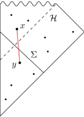
Definition 0 (Dou-Sorkin) - The pair { x, y } of elements of C is a horizon molecule if (i) y ∈ I

(Σ) ∩ I

( H ),

(ii) x ∈ I

(Σ) ∩ I

( H ),

(iii) | I[y, x] | = 0, i.e. y ≺ x is a link,

(iv) y is maximal in I

(Σ) ∩ I

( H ) and x is minimal in I

( H ).

x

y Σ

H

Figure 1.A Dou-Sorkin horizon molecule in a black hole spacetime.

An intuition of this definition is given in figure 1. The expected number of horizon molecules defined as such was shown to be proportional to the horizon area in the case of a 2-dimensional black hole spacetime. This promising result was soon undercut by the realisation that this definition yields a pathological divergence in d > 2. The intersection of the horizon with the future light-cone of y is an unbounded surface and ele- ments x are allowed to be sampled arbitrarily far away along this intersection. This IR divergence issue was pointed out in [6], where new definitions were introduced to cure this divergence. However, that make the mathematical handling of the subject lengthy and cumbersome.

Recent work from Barton et al [7] revisited the Dou-Sorkin proposal and extended the definition to more general causal horizons. The idea is to modify Definition 0 and require the hypersurface Σ to be strictly spacelike. The definition goes as follows. Let (M, g) be a globally hyperbolic spacetime with a Cauchy surface Σ. Let H be a causal horizon, defined as the boundary of the past of a future inextendible timelike curve γ, i.e. H := ∂I

(γ), and consider a random causal set ( C , ≺ ) generated on M through a Poisson sprinkling.

Definition 1 (Barton et al) - A horizon molecule is a pair of elements of C , { p

, p

} , such that (i) p

≺ p

,

(ii) p

∈ I

(Σ) ∩ I

( H ), (iii) p

∈ I

(Σ) ∩ I

( H ),

(iv) p

is the only element in I

(Σ) and in the future of p

.

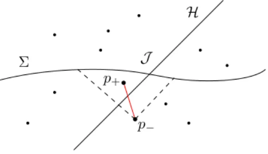
We give a graphical intuition on figure 2. This definition can be extended to a n-molecule { p

, p

, ..., p

}

by requiring p

≺ p

and { p

, ..., p

} to be the only elements in the future of p

and in I

(Σ). We are

going to use Definition 1 for the rest of this paper. It was shown that in the continuum limit, the expected

number of such defined horizon molecules limits to the area of the intersection of Σ and H up to a constant

dependent on the spacetime dimension. Mathematically, we restate (1) here:

ρ

lim

ρ

h H i = a

Z

J

dV

, (4)

where H is the random variable counting the number of horizon molecules in the sprinkling realisations, J = Σ ∩ H and dV

the surface measure on J .

p

p

Σ

H

J

Figure 2.Barton et al definition of horizon molecules with respect to a spacelike hypersurface Σ.

2.1. Horizon molecule counting with null hypersurfaces

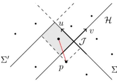
We now discuss the possibility to apply the Barton et al definition to a null hypersurface Σ. To avoid the IR divergence issues of Dou-Sorkin, we cannot use a straight null plane that renders the sprinkling domain unbounded. Instead, we shall put some regulators to bound the domain, or better to have it included as part of the null hypersurface. It’s natural to consider the case of Σ being a folded null plane and a downward light-cone respectively. The idea comes from the formulation of Einstein field equations solutions in term of a characteristic Cauchy problem [12]. Let us consider a spacetime ( M , g) and a null submanifold H defining a causal horizon. Let us then consider a null hypersurface Σ transverse to the horizon with a kink in the future of H . Call J the intersection J := H ∩ Σ. Let us assume a causal set C is sampled on ( M , g) through a Poisson sprinkling at density ρ. Then, the definition of horizon molecules given by Barton et al still holds and we are left with the setup of figure 3.

Σ H J p

p

Figure 3.We define the horizon molecule to be constrained into the past ofs$.

Defining now the expectation value of the number of horizon n-molecules as in [7], and calling p the element p

, one gets to the following identity

ρ

H

= ρ

Z

I−(J)

dV

(ρV

(p))

n! e

, (5)

where the volumes entering the integral are defined as

V

(p) :=vol I

(Σ) ∩ I

( H ) ∩ I

(p) , V (p) :=vol I

(Σ) ∩ I

(p)

. (6)

In order to make the computations more straightforward, it is useful to revert the time direction of our system, so that one lets p run in the future of the intersection hypersurface J . Equation (5) takes the form

ρ

H

= ρ

Z

I⁺(J)

dV

(ρV

(p))

n! e

. (7)

3. Minkowski spacetime

We will now probe our definition on a Minkowski d-dimensional spacetime. Let’s consider a d-dimensional Minkowski spacetime ( M

, η) with a submanifold H defining a Rindler causal horizon. We’re going to compute the expected number of horizon molecules with two distinct null hypersurface configurations, and find that they both agree with the area-law entropy.

3.1. Folded null planes

Let Σ be a null hypersurface transverse to the horizon and intersecting it in a co-dimension 2 surface J = Σ ∩ H . We set up the coordinates (v, u, y

) and let Σ be the v = 0 hypersurface and H the u = 0 one. We define the hypersurface Σ

given by u = λ, with λ > 0, which then lies in the future of H and it is parallel to the horizon. The union Σ

∪ Σ form a ∧ -shaped folded null plane, and we can ignore the leftover parts on the top.

Σ

Σ H J u v

p

Figure 4.A folded null plane crossing the horizon. The volumeV+, fis shaded

In this setup, the integrand of equation (7) is independent of y

. Thus one can write ρ

H

= Z

J

d

y I

(l, λ), (8)

with the function I

(l, λ) given by I

(l, λ) = l

n!

Z

0

dv Z

0

du (V

(u, v, λ))

e

, (9) Where we denoted with a f subscript the quantities evaluated on the Minkowski spacetime. As already said, for convenience we will work with a reversed time direction, so that p ∈ I

( J ). Then, the surface Σ

will be given by u = − λ. One can compute the volumes V

and V

in a coordinate system (x

, x

, y

) such that

v = x

+ x

√ 2 , u = x

− x

√ 2 , (10)

and so that the point p as x

= 0. Thus, V

:= V

− V

is given by the difference between the volume of

a cone of height x

and the volumes of two identical regions between the surfaces Σ (and H ) and a spacelike

surface x

= 0. One has

V

= Ω

d(d − 1) (x

)

− 2 Z

0

dx

Z

x^′0−x⁰

dx

Z √

(x⁰−x^′0)²−(x^′1)² 0

dR Z

S_d

−3

dΩ

R

= α

(x

)

, (11) where α

is a constant dependent on the dimension. This suggests volumes of the form of V

and V

are dependent only on the proper time between the origin and the point p. Thus, one gets

V

(u, v, λ) = α

(2v(u + λ))

, (12)

V

(u, v, λ) = α

(2v)

(u + λ)

− u

. (13)

Substituting equations (12) and (13) into (9) yields the result

I

(l, λ) = l

n!

Z

0

du Z

0

dv α

(2v)

(u + λ)

− u

e

d 2

,

= l

n!

Z

0

du α

d l

(u + λ)

− u

(u + λ)

Γ 2

d + n

,

= α

n!d Γ

2 d + n

Z

0

du

(u + λ)

− u

(u + λ)

. (14)

One can now evaluate the integral for different values of n, for example

I

= a

= α

d Γ

d + 2 d

H

2

, I

= a

= α

2d Γ

2 + 2 d

2H

2

− H

, (15)

with H

the n

harmonic number. We notice the result is independent of the Σ

hypersurface position with respect to the horizon, i.e. of the parameter λ. It follows that

ρ

lim

ρ

H

= a

Z

J

dV

(16)

holds in M

. This result is surprising as one would expect the locality argument given in Barton et al to fail in this setup. This is because in (5) the term exp( − ρV ) suppresses the contributions of points for which ρV ≫ 1, thus the points far from the intersection J in the case Σ is spacelike. With Σ null, contributions from points sampled arbitrarily close to Σ and arbitrarily far away from J will not be exponentially suppressed in the continuum limit. However, because of dimensional analysis, one can argue that the continuum limit of (8) must be dependent only of geometrical quantities at J . This is because of the symmetries of flat spacetime. One can always boost the system in the u direction to pull the surface Σ

arbitrarily close to H , thus the independence on λ, or points far in the past of J closer to the intersection.

3.2. Downward Light-cone

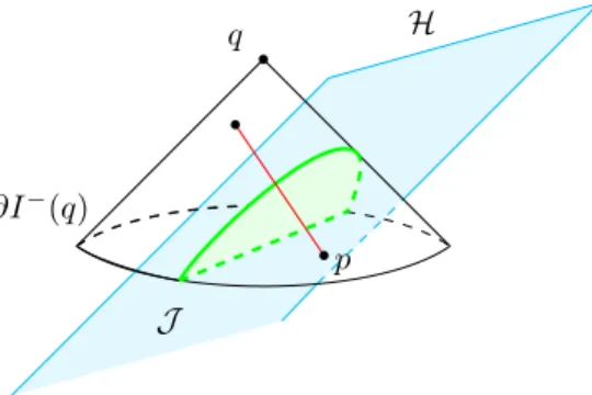
Now we consider Σ given by a downward light-cone, that is the boundary of the past of a point q ∈ I

( H ).

Then the horizon molecules will be sprinkled in the causal interval defined by the points p and q, i.e. I[p, q], see figure 5. Equation (5) remains the same, with the volumes given by

V

(p) :=vol I[p, q] ∩ I

( H ) ,

V (p) :=vol I[p, q]). (17)

q H

J

∂I

(q)

p

Figure 5.Sketch of a horizon molecules defined with respect to a downward light-cone.

We claim equation (16) holds in this configuration too. To supply evidence for this result, consider a causal diamond I[p, q] as defined above of proper length τ. In analogy to the previous calculations, suppose the time direction to be swapped, so that p ∈ I

( H ) and q ∈ I

( H ). By Lorentz invariance, one can compute its volume in a frame in which de diamond is spherically symmetric. Again we set up the coordinates system (x

, x

, y

) such that the origin sits in the middle of the diamond and we choose

p

= τ

2 , 0, ..., 0

, q

=

− τ

2 , 0, ..., 0

. (18)

Suppose then the horizon H is a Rindler horizon given by the condition x

= x

+ α, with α ∈ ( −

,

).

Therefore, one can write the volume of the region I

∩ I

( H ) as

V

=

Z

(

)

−^τ2

dx

Z

−x⁰−^τ2

dx

Z

q

(

)

dR Z

S_d

−3

dΩ

R

+ Z

−¹2

(

) dx

Z

x⁰−α

dx

Z

q

(

)

dR Z

Sd−3

dΩ

R

+

Z

(

)

0

dx

Z

x⁰−α

dx

Z

q

(

)

dR Z

S_d

−3

dΩ

R

.

(19)

These integrals are easily evaluated fixing the sprinkling spacetime dimension. For d = 4 one gets V

= π

48 τ(τ − α)(τ + 2α)

, (20)

which is consistent with the known formula for the volume of the whole diamond if α = 0 or α → τ /2. In order to be useful, the volume must be expressed in a Lorentz invariant way. The parameter α is not satisfactory, as it is proper to the reference frame in which the diamond is symmetric. Considering null coordinates v and u defined centred on q, one can see that the horizon intersects the lower diamond boundary at a point λ away from q in the u direction. This is useful to define the relation

λ = 1

√ 2 τ

2 + α

⇒ α

τ = √ 2 λ

τ − 1

2 . (21)

Identifying the quantity

2

= u

, τ = p

2u

v

and calling c the ratio c = λ/u

, one gets the form

V

= π 4 τ

1 2 c

− 1

3 c

= π(v

u

)

1 2

λ u

− 1 3

λ u

!

. (22)

We are now ready to estimate I

, which takes the form

I

(l, λ) = l

n!

Z

λ

du Z

0

dv π

(vu)

1 2

λ u

− 1 3

λ u

!

e

,

= ✘ ✘ ✘ ✘ l

n!

Z

λ

du ✘ ✘ ✘ l

λ

r 3 2π Γ

1 2 + n

u

(3u − 2λ)

,

=Γ 1

2 + n 1

2n!

r 3 2π

2

27

Γ(2n) Q

j=1

( − n − j) −

F

1, 1 − 2n, 1 − 3n;

3n

!

= a

. (23) We obtain a result independent on the discreteness scale and on the affine distance between the horizon and the point q. Claim (16) follows.

4. Curved spacetimes

The results of the previous sections suggest that the expected number of horizon molecules is indeed proportional to the area of the intersection between the horizon and Σ, when evaluated on a causal set approximating a Minkowski spacetime and once the continuum limit is taken. In generic curved spacetimes without any symmetries, however, it’s possible that the limit might receive some geometric contributions that is characterized by the scale λ introduced in the problem. Recall that in the two previous examples, λ is the affine distance between the fold, or the point q, and the horizon. Since λ itself can be arbitrarily rescaled, here we expect the contributions to have the invariant form combining λ and curvature tensors on the null hypersurface. For example, suppose the null congruence along Σ intersecting the horizon has zero expansion and shear at the intersection J , we ask how much does the cross section area expand/shrink at affine distance λ away from the J . Suppose λ is small as compared to the intrinsic curvature scale at J , the Raychaudhuri equation predicts the area increment to be approximately

∆A A = −

Z

Z

Ric(l, l) du du

. (24)

This dimensionless geometric quantity is of course invariant under reparameterization of the affine parame- ter, for that we also need to rescale the null generators l in accordance with the λ rescaling. For the problem at hand, the horizon molecule count can in principle depend on other geometric quantities that character- ized by λ, the intrinsic and extrinsic curvature data on the null hypersurface Σ. On the other hand, one might ask why the scale λ isn’t apparent in the two examples evaluated in Minkowski spacetime. In the folded null plane case, there is no intrinsic or extrinsic curvatures on Σ, so there is no curvature tensor to pair with λ. In the downward light-cone case, however, it does have non-zero extrinsic curvature. But the extrinsic curvature is directly given by 1/λ so it cancels with λ when we take the dimensionless combina- tion. We therefore expect a possibly different behaviour of the expected number of horizon molecules in not only in generic curved spacetimes, but also whenever the null hypersurface itself has some non-trivial extrin- sic curvatures. In this section, we shall only focus on the effect of the intrinsic curvature in curved spacetimes.

4.1. Folded null planes

Let us now consider a generic d-dimensional globally hyperbolic spacetime ( M , g) with a subregion H defining

a causal horizon. Let Σ be a null hypersurface transverse to the horizon and intersecting it in a co-dimension

2 surface J = Σ ∩ H . One can define coordinates adapted to this setting as follows [13]: choose first a set

of generic coordinates y

on an open subset ˜ J of J . On a neighbourhood of ˜ J in H let k

be a smooth

non-vanishing vector field such that the integral curves of k

are the null geodesic generators of H . Assume

k

is future directed. On an open neighbourhood ˜ H of ˜ J one can take as coordinates the (d − 1)-tuple (v, y

),

with v a parameter running on the integral curves of k

. At each point p ∈ H ˜ one can find a unique null

vector field l

normal to the spatial direction of H and such that k

l

= − 1, so that it is also future directed.

We can build coordinates (v, u, y

) on an open neighbourhood N of ˜ H with u the affine parameter along null geodesics generated by l

at the point (v, y

) on ˜ H . These coordinates are known in the literature as Gaussian Null coordinates (GNC). We define now a null hypersurface Σ

as the collection of the integral lines of the vector field k

, where k

is the vector field obtained by parallel transporting k

along the geodesics defining the surface Σ of a parameter s = λ.

Consider again a causal set ( C , ≺ ) sprinkled into M with a Poisson point process of density ρ = l

. In the tubular neighbourhood N ⊃ J in which GNC are constructed define the region

R

:= { p ∈ I

( J ) ∩ N | 0 < v(p) < − Λ, 0 < u(p) < − Λ } , (25) where Λ sets an intermediate scale between the discreteness length of C and the geometric length scale of the problem, i.e. l ≪ Λ ≪ L

. In order for the entropy to be a quantity local to the intersection J , one hopes to show equation (7) to be dominated by the integral on R

ρ

H

= ρ

Z

R^Λ

dV

(ρV

(p; λ))

n! e

+ . . . , (26)

with . . . denoting terms decaying exponentially fast in the limit of l → 0. As already discussed in the flat spacetime case, we believe this is not true in general in the case of Σ being a null hypersurface. The argument goes as follows: when v(p) ≤ − Λ and for all values of u(p), the volume V (p) will be large enough so that the exponential term in (5) effectively suppresses the contributions coming from this region in the continuum limit. In this case, one can suppose the set of values of V (p) foliates the integration domain and the bounds of [7], section IV.B, apply.

On the other hand, when u(p) ≤ − Λ this argument fails, as one can pick the point p to be close to the axis v(p) = 0 so that the volume V (p) is close to zero for values of u arbitrarily far in the past of J . Thus, the integral would in principle receive contributions coming from far away along the past light-cone of the intersection hypersurface. These contributions are not guaranteed to be convergent, as the coordinate u can run up to past infinity. In addition, they could also be ill defined, as the assumption for the curvature to be well behaved on a neighbourhood of the origin fails far away from it and caustics could in general appear along the light-cone. It is therefore difficult to give a formal treatment of the integral behaviour in this region. Therefore, we believe that the presence of information coming from far away in the past of the origin, even in the continuum limit, is a first indication the proposal of counting horizon molecules with a null hypersurface Σ is a flawed way to define entropy for a causal set.

One could however ask if the proposal of Barton et al together with a null hypersurface is still viable after considering Λ as a IR cutoff in the u direction, in order to exclude contributions from the far past of the intersection in the final count of the entropy. In the next subsection, where we consider a finite segment of null hypersurface attached with spacelike tails, such IR cutoff is automatically imposed by locality arguments as in Barton et al. We will therefore for the moment put it by hand and restrict our attention to the R

region. We shall explicitly write the (26) in GNC, always after inverting the time direction so to integrate p over the future of J ,

ρ

H

= ρ

n!

Z

J

d

y Z

0

dv Z

0

du p

− g(v, u, y) ρV

(v, u, y; λ)

e

+ . . .

= Z

J

d

y p

σ(y) I

(y; l, Λ, λ) + . . . ,

(27)

where we made explicit the dependence of the volumes on the parameter λ and we defined σ(y) the induced metric on J . This defines the function for any point y ∈ J ,

I

(y; l, Λ, λ) := l

n!

Z

dv Z

0

du s

− g(v, u, y)

σ(y) V

(v, u, y; λ)

e

. (28)

Here we can expand the above function in l up to the O (l) order. As compared to the previous calculations in the flat case where I

essentially localises to J , we expect here deviations due to the non-vanishing curvature tensors. Since I

is dimensionless, we need to contract any curvature tensors with objects with length dimensions. There are three independent scales in this problem: l, λ and Λ. They correspond to the discreteness scale, the distance between the fold and the horizon and the cutoff scale. By dimensional analysis and locality arguments, I

(y; l, Λ, λ) admits a small l expansion of the form

I

(y; l, Λ, λ) = a

+ X

j

c

F

(y, λ, Λ) + l X

i

b

G

(y, λ, Λ) + O (l

), (29) where a

, b

and c

are constants dependent on d and n. The set {G

(y, λ, Λ) } is the set of mutually independent geometric scalars of length dimension L

evaluated on the geodesic segment γ

(s). Likewise, the set {F

(y, λ, Λ) } is the set of mutually independent dimensionless geometric scalars evaluated on the geodesic segment γ

(s). These scalars can be obtained by from curvature tenors contracting with objects carrying scale λ or Λ. Equation (29) implies

lim

I

(y; l, Λ, λ) = a

+ X

j

c

F

(y, λ, Λ). (30) It is worth noting the difference between our analysis and [7] in the spacelike case. The case thereby discussed sees the volumes V and V

tend to the point y in the continuum limit and the integrand of I

is non-negligible in a neighbourhood of this point. The small l expansion is therefore dependent only on the geometric scalars evaluated at y. There are no other scales than l which can pair with the curvature tensors, so their I

does not have any such {F

(y, λ, Λ) } contributions. Their corresponding I

reads

I

(y; l, τ) = a

+ l X

i

b

G

(y) + O (l

) (31) where τ is a middle scale corresponding to our Λ and the curvature contributions are all localized to y ∈ J . In our null setup, however, the small l expansion must include geometric information evaluated on the geodesic segment from the horizon to the hypersurface Σ

, which carries with it additional scales λ and Λ.

Since such contributions {F

(y, λ, Λ) } are not forbidden on dimensional grounds, we expect generically part of these corrections to be present also in the continuum limit, which is summarised by equation (30). One can verify this by considering mild curvature perturbations close to J . These perturbations will enter the volume expressions V, V

in (28), and they generally do not cancel out. In the next subsection, we confirm this limiting behaviour in the downward light-cone example with explicit calculations.

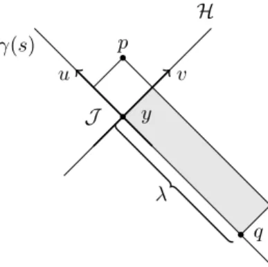
4.2. Downward Light-cone

We consider the same setup as in section 3.2. Consider Σ as the past-pointing light-cone of the point q, which is of affine distance λ away from J . The codimension-2 region J is defined as J := ∂I

(q) ∩ H . Again, the volumes of interest are

V

(p) :=vol I

∩ I

( H ) ,

V (p) :=vol I

). (32)

There will be a unique null geodesic γ passing through q, being transverse to the generators of the future

light-cone of p and crossing the horizon at a point y. Once again we will reverse the temporal direction to

perform the computations, so that p ∈ I

( H ) and q ∈ I

( H ). We will assume this geodesic to be affinely

parametrised so that γ(0) = y, γ( − λ) = q. In the continuum limit we expect the point p to shrink towards γ,

and the volumes V and V

shall tend to a skinny causal interval. Thus, we can set up a Null Fermi Normal

Coordinates system (v, u, y

) centred on this geodesic and with origin on J , where y

are carried from the

local coordinates of y in J . The horizon is given by the surface u = 0. A sketch of the coordinate system is

given in Figure 6.

H

J

v u

p

y

q λ

γ(s)

Figure 6.Time-reversed coordinate system in the skinny diamond setup. The volumeV₊ is shaded.

As in the previous section, the horizon molecules expectation value can be written as (27) in a tubular neighbourhood of J containing the point q and controlled by the parameter Λ. Thus we are once again left with the function I

(y; l, Λ, λ) defined as in equation (28). For the sake of simplicity we consider a spacetime dimension d = 4. We assume λ, Λ to be small relative to the local curvature scales such that we can obtain perturbative volume expansions for V and V

in u, v using the geometric data on γ. These were computed in the Appendix. Calling (v, u) the null coordinates of point p and fix a point y ∈ J , the volume expansion reads as (cf. (A.1))

V

(u, v, y; λ) = πτ

24 1 + 12 Z

−λ

du

(u − u

)

(u + λ)

(u

+ λ)

Z

−λ

dx Z

−λ

dx

(x

+ λ)R

(x

+ λ)

!

+ O ((u + λ)

, v

),

= V

1 + F (λ, u)

!

+ O ((u + λ)

, v

) (33)

where we define F(λ, u) to denote the integral. Analogously, defining c the ratio c = λ/(u+λ), the truncated diamond volume becomes

V₊⁽⁴⁾(u, v, y;λ) = πτ⁴ 4

c² 2 −c³

3

+πτ⁴ 2

Z 0

−λ

du^′(u^′+λ)²(u−u^′)² (u+λ)⁶

Z u^′

−λ

dx Z x

−λ

dx^′(x^′+λ)Ru′u′(x^′+λ) +O((u+λ)³, v³),

=V_+,f⁽⁴⁾ 1 + 2 c²

2 −c³ 3

−1Z 0

−λ

du^′(u^′+λ)²(u−u^′)² (u+λ)⁶

Z u^′

−λ

dx Z x

−λ

dx^′(x^′+λ)Ru′u′(x^′+λ)

!

+O((u+λ)³, v³),

=V_+,f⁽⁴⁾ 1 + ˜F(λ, u)

!

+O((u+λ)³, v³) (34)

where we define ˜ F (λ, u) to denote the integral.

Our goal is to show that the continuum limit of I

contains non-vanishing curvature terms. We can now insert those expansions in equation (28) and ignore henceforth the O (v

, (u + λ)

) tails as we assume λ, Λ are much smaller than the curvature scales.

In^(d)(y;l,Λ, λ) =l^−(4n+2) n!

Z Λ

0

dv ZΛ

0

du e^{−l−4Vf(4)(u,v,y;λ)}

V_+,f⁽⁴⁾(u, v, y;λ)n

1−l⁻⁴V_f⁽⁴⁾F(λ, u) +nF˜(λ, u)

! ,

=l^−(4n+2) n!

Z Λ

0

dv ZΛ

0

du e^{−l−4Vf(4)(u,v,y;λ)}

V_+,f⁽⁴⁾(u, v, y;λ)n

−l^−(4n+2) n!

Z Λ

0

dv Z Λ

0

du e^{−l−4Vf(4)(u,v,y;λ)}

V_+,f⁽⁴⁾(u, v, y;λ)n

l⁻⁴V_f⁽⁴⁾F(λ, u)

+l^−(4n+2) n!

Z Λ

0

dv Z Λ

0

du e^−l−4V

(4)

f (u,v,y;λ)

V_+,f⁽⁴⁾(u, v, y;λ)n

nF˜(λ, u). (35)

The first term of equation (35) is the all-flat term computed in section 3.2. Assuming the integrals in the second and third lines are suppressed exponentially fast for v > Λ, we can write

− l

n!

Z

dv Z

0

du e

V

(u, v, y; λ)

l

V

(u, v, y; λ)F (λ, u),

= − q

2π

Γ

+ n Γ (n + 1)

Z

du F(λ, u) u + λ 3

λ u + λ

− 2 λ

u + λ

!

+ ..., (36)

where ... denote terms decaying exponentially fast in the limit l → 0. Analogously, the third term becomes l

(n − 1)!

Z

dv Z

0

du e

V

(u, v, y; λ)

F ˜ (λ, u),

= q

2π

Γ

+ n Γ (n)

Z

du F(λ, u) ˜ u + λ 3

λ u + λ

− 2 λ

u + λ

!

+ .... (37)

We can now evaluate F (λ, u) and ˜ F(λ, u). For simplicity we assume that R

(y) = R (y) is constant over u, which is good enough to support our claim. Thus,

F(λ, u) = R (y)

15 (u + λ)

, F ˜ (λ, u) = R (y) 90

1 2

λ u + λ

− 1 3

λ u + λ

!

λ

(λ

+ 5λu + 10u

) (λ + u)

. (38) Inserting now (38) into (36) and (37) we get

− q

2π

Γ

+ n Γ (n + 1)

Z

du F (λ, u) u + λ 3

λ u + λ

− 2 λ

u + λ

!

,

= − q

2π

Γ

+ n R (y) 15Γ (n + 1)

Z

du (u + λ) 3 λ

u + λ

− 2 λ

u + λ

!

∼

( R (y)λ

log(λ + Λ) if n = 1 R (y)λ

f (λ, Λ) if n > 1,

(39) with f (λ, Λ) ∼ O (1) if Λ ≫ λ; and

q

2π

Γ

+ n Γ (n)

Z

du F ˜ (λ, u) u + λ 3

λ u + λ

− 2 λ

u + λ

!

,

= q

2π

Γ

+ n R (y) 15Γ (n)

Z

du λ

(λ

+ 5λu + 10u

) (λ + u)

λ

(λ + 3u) (λ + u)

∼ R (y)[λ

+ ˜ f (λ, Λ)], (40)

with ˜ f (λ, Λ) → 0 if Λ ≫ λ. Thus, the horizon molecules expectation value admits a continuum limit of the

form (30), i.e.

l

lim

I

(y; l, Λ, λ) = a

+ R (y)c

(λ, Λ) + · · · (41) where the · · · contains other curvature terms that are higher order in the volume expansions, e.g. ∼ R

λ

. We see that the limit is not local to the intersection J . We thus conclude that this horizon molecule definition does not yield a well behaved area law for the entropy when evaluated on a null hypersurface crossing a causal horizon.

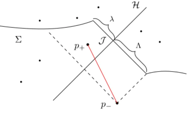
4.3. Hypersurfaces of mixed signature

So far we have studied the particular example of downward light-cone and shown that horizon molecule count in the continuum limit is not proportional to the horizon area, but rather it is also influenced by the curvature data on the null surface. It can be traced down to the fact that the dominant region of contribution localizes to the entire neighbourhood of bounded null segment, rather than J as in the spacelike case. As we argued from the dimensional grounds, we believe this dependence is generic whenever we have a null hypersurface crossing the horizon. In particular, this can even be a piece of null segment that is part of an elsewhere spacelike hypersurface as illustrated in figure 7.

λ

Λ

p

p

Σ

H

J

Figure 7.Mixed signature hypersurface Σ which is everywhere spacelike except for a null segment crossing the horizon. The contribution from the region beyond the dashed line is exponentially suppressed.

Consider such a hypersurface of mixed signature, whose null segments spans a parameter distance λ+Λ. The advantage of this setup as opposed to the infinitely past-extending null hypersurface is that the spacelike sections provide natural IR cutoffs as we alluded to earlier. One can apply the locality argument of Barton et al up to the point where the local neighbourhood to J crosses the spacelike sections and contains mostly the null segments. (See the shaded region in Figure 7.) This defines for us a cutoff scale Λ beyond which the contribution is exponentially suppressed. Then we just need to compute (28) and it’s clear from above arguments that generically this integral is not going to localize to J as we approach the continuum limit.

Note that the hypersurface signature at the intersection J needs not be everywhere null for this argument to hold. The null segment can also have finite extent in the transverse direction, which is enough to distort the area law behaviour.

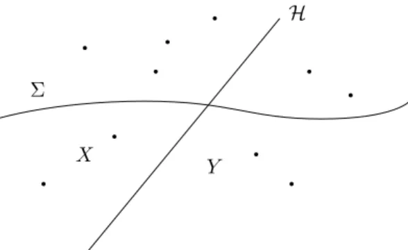
5. Entropy from SMI

In the previous sections, we discussed the issues of applying the horizon molecules program to null Σ hyper-

surfaces. To still be able to properly define a horizon entropy in this situation, we now focus on the spacetime

mutual information (SMI) proposal. Take a spacetime ( M , g) approximated by a causal set ( C , ≺ ). A causal

horizon H can be given in the causal set, mapping a future-inextensible timelike curve in M to a future-

infinite chain of causal set elements. Considering then a non-timelike hypersurface Σ crossing the horizon,

which can also be defined in similar ways in a causal set, one is left with two regions X and Y laying in the

past of Σ and separated by H (Figure 8). Defining Y as the region at the past of the horizon, we see that it

will evolve independently of X as far as causality is preserved.

Σ

H

X Y

Figure 8.Partition of a spacetime and of a causal set by a causal horizonH.

In [14], this latest fact together with the properties of the Causal Set action led to define a quantity that can be a candidate for a horizon entropy. Recall the definition of the Benincasa-Dowker action for causal sets in dimension 4 [15, 16],

S

(C) = 4

√ 6l

h N − N

+ 9N

− 16N

+ 8N

i , (42)

where N is the cardinality of the causal set, l is a fundamental length, N

the number of m-inclusive intervals in C . If one partitions the causal set C into two subsets X and Y so that C = X ∪ Y and X ∩ Y = ∅ the action, noted from now on by S for shortness, will not be local and additive, i.e.

S[ C ] 6 = S[X ] + S[Y ]. (43)

Taking the cue from thermodynamics and information theory, one can therefore define the Spacetime Mutual Information (SMI) between two regions X and Y as

I

[X, Y ] :=

l

l

S

[X] + S

[Y ] − S

[ C ]

. (44)

In [14] is conjectured that the expectation value of the SMI tends, in the continuum limit, to the volume of the intersection between the horizon and the hypersurface Σ, i.e. J := H ∩ Σ, times a dimension-dependent constant,

l

lim

D I

[X, Y ] E

= b

vol( J ) l

. (45)

This would then suggest the SMI gives the continuum area law for the horizon entropy, at least from a kinematical point of view. The evidence to support this conjecture has been collected from numerical simulations and it seems to be consistent with the expectations. We shall thereby consider a simple setup with a causal interval in 4D Minkowski spacetime and analytically confirm (45):

lim

D I

[X, Y ] E

= vol( J )

l

. (46)

with b

= 1.

We demonstrate the calculations in Minkowski spacetime ( M

, η). We suppose the spacetime is partitioned

by a Rindler causal horizon H . We pick two points in M

, p and q, sitting in the past and in the future of

the horizon respectively. And we consider the causal diamond I[p, q] between these two points. We define

Null Fermi Normal Coordinates, set up as in the Appendix. From the point p, we shoot a null geodesic γ(p, o) of affine length L. At o, a second null geodesic orthogonal to γ(p, o) is shot, defining γ

(o, q), with q at an affine parameter s along it. This defines the causal interval I[p, q]. We then define Null Fermi Normal Coordinates adapted to the geodesic γ(p, o), (x

, x

, r, θ). Note the transverse spatial part is described in spherical coordinates. Thus, the metric reads

ds

= − 2dx

dx

+ dr

+ r

dθ

(47)

and the relevant points in our construction have coordinates p

= (0, ..., 0), o

= (L, 0, ..., 0) and q

= (L, s, 0, ..., 0). The horizon is given by the hypersurface H = { (cL, x

, r, θ) } , with c ∈ (0, 1).

Consider now as usual a causal set C sprinkled in the interval I[p, q] at a density ρ. In this setup, the causal diamond is partitioned by the horizon into two regions X and Y , with X lying in the future of the horizon and Y in its past. The computation of the spacetime mutual information between these two regions can be tackled in different ways, either looking for N

(X, Y |C ) or by computing the action of the regions X and Y separately. The first approach turns out to be difficult, especially because of the reduced spherical symmetry of the problem due to the presence of the horizon as a boundary of X and Y . Looking for the action on the two subregions is easier, especially noticing that the region X has the horizon sitting only on the past boundary. The inner integral in the usual action evaluation is thus blind to the presence of the horizon and can be straightforwardly carried out considering a properly boosted causal diamond. One has

D N

(X) E

= ρ

Z

X

d

x Z

X∩I⁺(x)

d

y e

= ρ

X

n

− ρ

n!

Z

X

d

x πΓ(2n + 4)

4(n + 1)Γ(2n + 4) τ

. (48) The integration measure over X becomes in NFNC

Z

X

d

x = Z

cL

dx

Z

0

dr r Z

x⁻_min

dx

Z

S1

dθ, (49)

with

x

= r

2x

, x

= r

2(x

− L) + s, (50)

fixing the boundaries of the causal diamond and r

= p

2sx

(1 − x

/L) is the radius at which the upper and lower light-cones intersect. Furthermore, the proper time between x and q is given by

τ

= 2(L − x

)(s − x

) − r

. (51)

Equation (48) therefore becomes

D N

(X ) E

= ρ

X

n

− ρ

n!

Z

X

d

x πΓ(2n + 4)

4(n + 1)Γ(2n + 4) τ

,

= ρ

X

n

− ρ

n!

π

Γ(2n + 4) 2(n + 1)Γ(2n + 4)

Z

dx

Z

0

dr

· Z

x⁻_min

dx

r 2(L − x

)(s − x

) − r

,

= ρ

X

n

− ρ

n!

π

(1 + 2c(n + 2))(1 − c)

2

(n + 1)

(n + 2)

(2n + 1)(2n + 3)

(2n + 5) (τ

)

,

= X

n

( − N

)

n!

9 (1 + 2c(n + 2))

(1 + 2c)

(n + 1)

(n + 2)

(2n + 1)(2n + 3)

(2n + 5) . (52) In the third equality we used the identity τ

= 2Ls and in the last step we wrote the sum as a function of N

, i.e. the number of causal set elements sprinkled in the region X , which is given by

N

= ρ vol(X ) = ρ π τ

24 (1 − c)

(1 + 2c). (53)

After differentiation of equation (52) with respect to ρ to obtain the number of m − inclusive intervals in X , we are ready to insert the results into the definition of the causal set action in 4 dimensions

1

~

D S

(X ) E

= α

l l

N

− D

N

(X ) E + 9 D

N

(X) E

− 16 D

N

(X) E + 8 D

N

(X ) E

. (54) Taking the continuum limit, i.e. sending N

to infinity, one gets that the action has a leading contribution

1

~ D

S

(X ) E

∼ l

l

2 p

6π N

(1 + c)

√ 1 + 2c . (55)

Inserting equation (53) into (55) we can express the continuum limit as a function of the number of points sprinkled on the whole I[p, q] interval, which then reads

1

~

D S

(X) E

∼ l

l

2 √

6π N (1 − c

). (56)

We can now use the relation between N and the proper length of the interval N = ρV = ρ ζ

τ

= ρ π

24 τ

(57)

and write the continuum limit of the action as

ρ

lim

1

~

D S

(X ) E

= 1

l

πτ

(1 − c

). (58)

From this result we can easily infer the continuum limit of the action evaluated on the region Y . The BD action is invariant under time reversion, then when evaluated on the region Y , its value will only depend on the position of the horizon, i.e. c → 1 − c. We infer

ρ

lim

1

~

D S

(Y ) E

= 1

l

πτ

c(2 − c). (59)

We are now able compute the SMI between the regions X and Y . Recalling

ρ

lim

1

~

D S

( C ) E

= 1

l

πτ

, (60)

one has, using (44),

D I

[X, Y ] E

= 2

l

πτ

c(1 − c). (61)

One shall now compare this result to the volume of the dimension 2 joint of the region X. This joint is

composed of three sections: the intersection of the future light-cone of p with the past light-cone of q J

,

and the intersections J

, J

between both those light-cones and the horizon H . These are named after their

q

p X

Y J

J

J

H

Figure 9. Three dimensional I[p, q] diamond cut by an horizonH. The black bold line is the null-null joint section contributing to the action of regionX. The green bold arch is the cone-horizon joint section contributing in regionX, whereas the red arch contributes in regionY.

colour labels in Figure 9.

We start considering the cone-cone piece of the joint J

(i.e the black bold curve in Figure 9). For a diamond of proper length τ, boosted such that it is spherically symmetric around the time direction, the intersection of the light-cones emanating from p and q is a sphere of radius τ /2. Considering now the spacetime to be mapped by a chart (x

, x

, r, θ) centred in the middle of the diamond, one can parametrise the joint as the surface

J

(x

, θ) = 0, x

, r

τ 2

− x

sin θ, r

τ 2

− x

cos θ

!

. (62)

One can then see the joint as a surface of revolution around the segment x

∈ [ − τ /2, τ /2]. The truncation induced by the horizon limits the span of the coordinate x

to x

∈ [ − τ /2, τ /2 − √

2λ]. Thus, the surface area of the joint is given by

vol ( J

) = Z

0

dθ

Z

x1,min

dx

r(x

) p

1 + r

(x

)

,

= Z

0

dθ

Z

−^τ2

dx

r τ

2

− x

v u u u t 1 +



 x

q

− x





2

,

= πτ

1 −

√ 2λ τ

!

= πτ

(1 − c) . (63)

The intersection of the light-cones with the horizon are dimension 2 null surfaces in M

, in red and green on Figure 9. In order to compute their surface area, we consider the coordinate chart (t, x, y, z) on M and first look at the future light-cone L

, up to a time coordinate t ≤ τ /2. In this coordinate, the horizon is at H = { t − x = √

2λ } . We can therefore find a condition for x, i.e. x = t − √

2λ. We can now impose the light-cone definition to the 4-tuple (t, t − √

2λ, y, z)

0 = − t

+ x

+ y

+ z

⇒ y

+ z

= 2 √

2tλ − 2λ. (64)