The massive dirac equation in Kerr Geometry: Separability in Eddington- Finkelstein-type coordinates and

Universit¨ at Regensburg Mathematik

The massive dirac equation in Kerr Geometry: Separability in Eddington- Finkelstein-type coordinates and

asymptotics

Christian R¨ oken

Preprint Nr. 12/2015

Eddington-Finkelstein-Type Coordinates and Asymptotics

Christian R¨oken

Universit¨at Regensburg, Fakult¨at f¨ur Mathematik, 93040 Regensburg, Germany (Dated: June 29, 2015)

ABSTRACT. The separability of the massive Dirac equation in a rotating Kerr black hole back- ground in advanced Eddington-Finkelstein-type coordinates is shown. To this end, the Kerr space- time is described in the framework of the Newman-Penrose formalism by a local Carter tetrad, and the Dirac wave functions are given on a spin bundle in a chiral Newman-Penrose dyad representation.

Applying mode analysis techniques, the Dirac equation is separated into coupled systems of radial and angular ordinary differential equations. Asymptotic radial solutions at infinity and the event and Cauchy horizons are explicitly derived and, by means of error estimates, the decay properties are analyzed. Solutions of the angular ordinary differential equations matching the Chandrasekhar-Page equation are discussed. These solutions are used in order to study the scattering of Dirac waves by the gravitational field of a Kerr black hole for an observer described by a frame without coordinate singularities at the inner horizon boundaries such that Dirac waves can be seen to actually cross the event horizon.

Contents

I. Introduction 2

II. Preliminaries 3

A. General Relativity in the Newman-Penrose Formalism 3

B. The General Relativistic Dirac Equation in the Newman-Penrose Formalism 5 III. Newman-Penrose Representation of Kerr Geometry in Advanced Eddington-Finkelstein-Type

Coordinates 6

IV. The Dirac Equation in the Extended Kerr Black Hole Spacetime 14

A. Mode Ansatz and Separability 14

B. Asymptotic Analysis of Radial Solutions at Infinity 15

C. Asymptotic Analysis of Radial Solutions at the Event Horizon 18

D. Asymptotic Analysis of Radial Solutions at the Cauchy Horizon 20

E. Angular Solutions 20

V. Scattering of Dirac Waves by the Gravitational Field of a Kerr Black Hole 21

VI. Summary and Outlook 22

e-mail: christian.roeken@mathematik.uni-regensburg.de

arXiv:1506.08038v1 [gr-qc] 26 Jun 2015

Acknowledgments 23

References 23

I. INTRODUCTION

Over the last five decades, the dynamics of relativistic spin-¹₂ fermions (Dirac waves) in black hole spacetimes was studied extensively using different approaches. The probably most established approach is based on Chan- drasekhar’s mode analysis [6–8, 12, 23, 39], where the massive Dirac equation in a Kerr-Newman black hole back- ground geometry is separated by means of time and azimuthal angle modes and rewritten in terms of 1-dimensional radial wave equations and coupled angular ordinary differential equations (ODEs). Within this framework, the asymptotic behavior of solutions of the Dirac equation can be studied, giving further rise to spectral estimates [17].

This opened up the possibility to study many physical processes like the emission and absorption of Dirac waves by black holes or the stability of black hole spacetimes under fermionic field perturbations [3, 22, 28, 30–32, 34–

36]. Moreover, the dynamics of Dirac waves was analyzed in the framework of scattering theory [1, 5, 9, 10, 20].

More recently, a functional analytic construction, that is, an integral representation of the Dirac propagator in the Cauchy problem formulation of the Dirac equation [16, 18], was used.

The basis of the mode analysis approach is Chandrasekhar’s famous finding that the Dirac equation in a Kerr black hole background given in Boyer-Lindquist coordinates is separable, which was worked out in his original article from 1976 [6] and led to a major breakthrough in the field. At that time, this remarkable result came a bit as a surprise because the Dirac system of coupled first-order partial differential equations (PDEs) was not expected to be separable. Despite the tremendous impact of this finding, the validity of the solutions is naturally restricted to those regions of the Kerr spacetime where the Boyer-Lindquist coordinates are well-defined, and since they have coordinate singularities at the Cauchy horizon and the event horizon, respectively, the description of Dirac waves in the vicinity of these horizons is ill-defined, i.e., Dirac waves cannot be propagated across these inner boundary surfaces. This poses a profound problem in all studies which rely on a proper description of their dynamics near and across these horizons as in the transmission and reflection of incident waves at the gravitational field of the black hole evaluated at the event horizon.

In this article, this problem is resolved by using an analytic extension of the Boyer-Lindquist coordinate frame to an advanced Eddington-Finkelstein-type coordinate system which is well-defined at the Cauchy and event horizons (for another coordinate system with similar characteristics, called Doran coordinates, see [13]). This coordinate system covers the interior and exterior black hole regions and yields a smooth transition of Dirac waves between them. Based on this description of Kerr geometry, a proper mode analysis of Dirac waves is conducted as follows.

Firstly, Kerr geometry is described in the Newman-Penrose formalism by a Carter tetrad in advanced Eddington- Finkelstein-type coordinates. Secondly, the associated spin coefficients are calculated and by their means, one formulates the Dirac equation in the chiral representation in terms of two bi-spinor equations with a Newman- Penrose dyad basis for the spinor space. In this form, the Dirac equation has no irregular singularities on the event and Cauchy horizons. Considering a factorization of the Dirac waves in coordinate time and azimuthal angle modes, separability of the Dirac equation in the advanced Eddington-Finkelstein-type coordinates into radial and polar angular ODEs is shown. Asymptotic radial solutions at infinity and at the event and Cauchy horizons are determined. Moreover, error estimates for these asymptotic solutions are given, and it is proven that the errors have suitable decay properties. The angular ODEs yield the usual Chandrasekhar-Page equation. The corresponding set of eigenfunctions and the discrete, non-degenerate spectrum of eigenvalues are briefly, however appropriately,

discussed. Finally, the radial asymptotics at infinity and at the event horizon are applied to the physical problem of scattering of Dirac waves by the gravitational field of a Kerr black hole. More precisely, the net current of incident Dirac waves, which emerge from space-like infinity, expressed in terms of the reflection and transmission coefficients, is considered and evaluated at infinity and at the event horizon. Note that here, in contrast to the usual treatment in Boyer-Lindquist coordinates, where the Dirac waves are observed to approach the event horizon only asymptotically, the Dirac waves are seen to actually cross the event horizon. Furthermore, due to the boundary conditions for the scattering problem, the discontinuity in the radial Dirac current across the event horizon coming from a horizon contribution to the Dirac waves, is removed. The well-known main results of the scattering problem in a Boyer-Lindquist representation are reproduced in this context, namely that the conserved net current stays positive across the event horizon and that superradiance cannot occur.

This work provides the fundamental quantities necessary for the construction of an integral representation of the Dirac propagator in advanced Eddington-Finkelstein-type coordinates acting on Dirac waves with compact support in the black hole interior and exterior regions, which is presented in a separate article [33].

II. PRELIMINARIES

In this section, a general overview of the local Newman-Penrose null tetrad formalism of general relativity and of the local dyad Newman-Penrose formulation for spinors for a description of the general relativistic Dirac equation are given. These formulations are very well suited for the analysis of radiative transport in curved spacetimes, especially Dirac wave propagation in a (vacuum) Kerr black hole background, because they can be chosen to reflect underlying symmetries and can be adapted to certain aspects of the spacetime, which subsequently leads to a reduction in the number of conditional equations and simplified expressions for geometric quantities.

A. General Relativity in the Newman-Penrose Formalism

Let (M,g) be a Lorentzian 4-manifold endowed with an affine connectionω, the unique, torsion-free Levi-Civita connection, and dual basis (eµ) and (e^µ),µ∈ {1,2,3,4}, on sections of the tangent and cotangent bundlesTMand TM^?, respectively. In addition, one sets up a flat (orthonormal or null) frame bundleFMand a spin bundleSM onM. The basis of the local frames of the fibers inFMat each point of spacetime consists of four vectors e(a)

, a ∈ {1,2,3,4}, and the basis of the corresponding dual frames are denoted by e^(a)

. The basis vectors of these internal frame bundles are related to the basis vectors of the tangent and cotangent bundles viae_(a)=e^µ_(a)e_µ and e^(a)=eµ^(a)e^µ, wheree^µ_(a) is an invertible linear map, namely a (4×4)-matrix, from TM toFM. Geometrical structures in the framework of general relativity can be described in terms of these local tetrad frames since they encode the same information as the metric tensor on the tangent bundle [37].

In the Newman-Penrose formalism [26], the tetrad basis consists of two real null vectors, l = e₍₀₎ =e⁽¹⁾ and n=e₍₁₎=e⁽⁰⁾, and a complex conjugate pair,m=e₍₂₎=−e⁽³⁾ andm=e₍₃₎=−e⁽²⁾. A Newman-Penrose frame has to fulfill the null conditions

l·l=n·n=m·m=m·m= 0, (1) the orthogonality conditions

l·m=l·m=n·m=n·m= 0, (2)

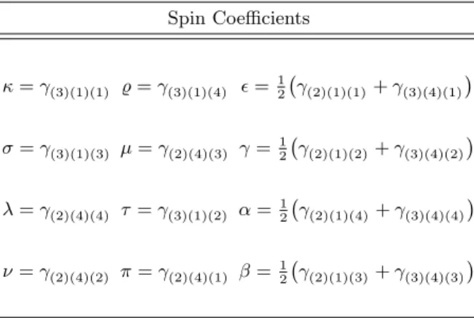
Spin Coefficients

κ=γ_(3)(1)(1) %=γ_(3)(1)(4) =¹₂ γ_(2)(1)(1)+γ_(3)(4)(1)

σ=γ_(3)(1)(3) µ=γ_(2)(4)(3) γ=¹₂ γ_(2)(1)(2)+γ_(3)(4)(2)

λ=γ_(2)(4)(4) τ =γ_(3)(1)(2) α=¹₂ γ_(2)(1)(4)+γ_(3)(4)(4)

ν=γ_(2)(4)(2) π=γ_(2)(4)(1) β= ¹₂ γ_(2)(1)(3)+γ_(3)(4)(3)

TABLE I: Various spin coefficients of the Newman-Penrose formalism expressed in terms of the Ricci rotation coefficients.

and the cross-normalization conditions (depending on the signature convention)

l·n=−m·m= 1. (3)

The metric gin terms of the Newman-Penrose null basis vectors becomes g=l⊗n+n⊗l−m⊗m−m⊗m.

Acting with this metric on the dual Newman-Penrose basis vectors, one obtains the local, non-degenerate, constant metricηon the null frame bundle

η=g

e^(a), e^(b)

=













0 1 0 0

1 0 0 0

0 0 0 −1 0 0 −1 0











 .

Since the connectionωis torsion-free, the first Maurer-Cartan equation of structure reduces to de^µ+ω^µ_ν∧e^ν = 0.

In the tetrad formulation this equation becomes

de^(a)=γ^(a)_(b)(c)e^(b)∧e^(c),

where the symbols γ^(a)_(b)(c) denote the Ricci rotation coefficients which are related to the Levi-Civita connection by means of the formula

γ^(a)_(b)(c)e^(c)=e_µ^(a)de^µ_(b)+e_µ^(a)e^ν_(b)ω^µ_ν.

The Ricci rotation coefficients in the framework of the Newman-Penrose formalism are called spin coefficients and designated by the twelve symbols given in TABLE I. They represent the Levi-Civita connection on the internal frame bundle described in terms of a Newman-Penrose null basis. The first Maurer-Cartan equation of structure in this formalism reads

dl= 2<()n∧l−2n∧ <(κm)−2l∧ < [τ−α−β]m

+ 2i=(%)m∧m

dn= 2<(γ)n∧l−2n∧ < [α+β−π]m

+ 2l∧ <(νm) + 2i=(µ)m∧m (4)

dm= dm

= (π+τ)n∧l+ 2i=()−%

n∧m−σn∧m+ µ+ 2i=(γ)

l∧m+λl∧m−(α−β)m∧m.

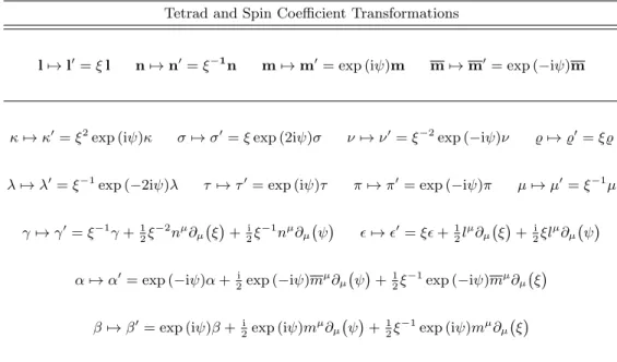
Tetrad and Spin Coefficient Transformations

l7→l⁰=ξl n7→n⁰=ξ⁻¹n m7→m⁰= exp (iψ)m m7→m⁰= exp (−iψ)m

κ7→κ⁰=ξ²exp (iψ)κ σ7→σ⁰=ξexp (2iψ)σ ν7→ν⁰=ξ⁻²exp (−iψ)ν %7→%⁰=ξ%

λ7→λ⁰=ξ⁻¹exp (−2iψ)λ τ7→τ⁰= exp (iψ)τ π7→π⁰= exp (−iψ)π µ7→µ⁰=ξ⁻¹µ

γ7→γ⁰=ξ⁻¹γ+¹₂ξ⁻²n^µ∂µ ξ

+₂ⁱξ⁻¹n^µ∂µ ψ

7→⁰=ξ+¹₂l^µ∂µ ξ

+₂ⁱξl^µ∂µ ψ

α7→α⁰= exp (−iψ)α+₂ⁱexp (−iψ)m^µ∂µ ψ

+¹₂ξ⁻¹exp (−iψ)m^µ∂µ ξ

β7→β⁰= exp (iψ)β+₂ⁱexp (iψ)m^µ∂µ ψ

+¹₂ξ⁻¹exp (iψ)m^µ∂µ ξ

TABLE II: Effect of a type III local Lorentz transformation on the Newman-Penrose basis vectors and the spin coefficients.

The quantitiesξ∈R\{0}andψ∈Rare functions depending on the spacetime coordinatesx^µ.

The relevant transformations that are applied on the Newman-Penrose tetrad frame in this study are elements of the 2-parameter subgroup of the 6-parameter group of local Lorentz transformations known as type III or spin-boost Lorentz transformations. These renormalize the real Newman-Penrose vectors l andn, but leave their directions unchanged, and rotate the complex conjugate pairmandmby an angleψin the (m,m)-plane. The effect of these transformations on the Newman-Penrose basis vectors and the spin coefficients is shown in TABLE II. There are various aspects of the Newman-Penrose formalism that are not explicitly discussed in this subsection such as the different types of local Lorentz transformations or the Weyl scalars with their algebraic classification because here, they are of no relevance. They can be found elsewhere in the literature. The interested reader may be referred to [27, 29].

B. The General Relativistic Dirac Equation in the Newman-Penrose Formalism

The general relativistic, massive Dirac equation without an external potential [19, 38] is given by the homogeneous linear first-order PDE system

γ^µ∇µ+ im

Ψ(x^µ) = 0,

where theγ^µ denote the general relativistic Dirac matrices which satisfy the anticommutator relations{γ^µ, γ^ν}= 2g^µνid_C4, Ψ(x^µ) the Dirac 4-spinor on sections of the spin bundle SM, ∇µ the covariant derivative on sections of the tangent bundle TM, and m the fermion rest mass. Using the chiral bi-spinor representation of the Dirac 4-spinors and matrices in terms of the 2-component spinorsP^A andQB˙ and the Hermitian (2×2)-Infeld-van der Waerden symbols σ^µ

AB˙ [20]

Ψ = P^A QB˙

!

and γ^µ=√

2 0 σ^µAB˙

σ^µ

AB˙

T

0

!

with A∈ {1,2} and B˙ ∈ {˙1,˙2},

one obtains the following 2-spinor form of the Dirac equation

∇BA˙ P^A+ iµ_?QB˙ = 0

∇BA˙ Q^A+ iµ?PB˙ = 0,

(5)

whereµ_?:=m/√

2 and∇_AB˙ =σ^µ

AB˙∇_µ. Note that a dot over an index indicates that the index transforms via the complex conjugated transformation. Introducing a local dyad basis ζ^(k),k∈ {1,2}, on the spin bundle analogous to the tetrad representation of the tangent bundle, the local Dirac 2-spinors O^(m) in terms of the 2-spinors O^A read O^(m)=ζ^(m)_AO^A, where ζ^(m)_A is an invertible (2×2)-matrix. In this dyad formalism, the spinor covariant derivative acting on the local 2-spinorO^(m)becomes

∇_{(k)( ˙l)}O^(m)=ζ^A_(k)ζ^B˙_{( ˙l)}ζ^(m)_C∇_AB˙O^C =∂_{(k)( ˙l)}O^(m)+ Γ^(m)

(n)(k)( ˙l)O⁽ⁿ⁾

with the spinor partial derivative

∂_{(k)( ˙l)}=σ^µ

(k)( ˙l)∂_µ and the spin coefficients

Γ^(m)

(n)(k)( ˙l)= Γ^{(m)( ˙o)}

(n)( ˙o)(k)( ˙l)=√

2^{(m)(q)( ˙o)( ˙p)}σ^µ_{(q)( ˙p)}σ^ν_{(n)( ˙o)}σ^λ_{(k)( ˙l)}e_µ^(a)e_ν^(b)e_λ^(c)γ_(a)(b)(c). (6) The 2-dimensional Levi-Civita symbolacts as skew metric on the fibers of the local spin bundle and the Infeld-van der Waerden symbols in the Newman-Penrose spinor formalism yield

σ^µ

(k)( ˙l)= l^µ m^µ m^µ n^µ

!

. (7)

With the spin coefficients of the dyad formalism (6) expressed in terms of the spin coefficients of the tetrad formalism (TABLE I), the Infeld-van der Waerden symbols (7), and the functions F1 :=P⁽⁰⁾,F2 :=P⁽¹⁾,G1 :=Q^{( ˙1)}, and G2:=−Q^{( ˙0)}, the general relativistic Dirac equation (5) in the Newman-Penrose formalism is given in the following form

(l^µ∂_µ+ε−%)F1+ (m^µ∂_µ+π−α)F2= iµ_?G1

(n^µ∂µ+µ−γ)F2+ (m^µ∂µ+β−τ)F1= iµ?G2

(l^µ∂µ+ε−%)G2−(m^µ∂µ+π−α)G1= iµ?F2

(n^µ∂_µ+µ−γ)G1−(m^µ∂_µ+β−τ)G2= iµ_?F1.

(8)

III. NEWMAN-PENROSE REPRESENTATION OF KERR GEOMETRY IN ADVANCED EDDINGTON-FINKELSTEIN-TYPE COORDINATES

Kerr geometry [24] is an asymptotically flat Lorentzian 4-manifold (M,g) with inner event and Cauchy horizon inner boundaries and with topology S²×R². It consists of a differentiable manifold Mand a stationary, axisymmetric Lorentzian metric g with signature (1,3), which is given in Boyer-Lindquist coordinates (t, r, θ, ϕ) [2], wheret ∈ R, r∈R>0, θ∈[0, π], andϕ∈[0,2π), by

g=∆

Σ dt−asin²(θ)dϕ

⊗ dt−asin²(θ)dϕ

−sin²(θ)

Σ [r²+a²]dϕ−adt

⊗ [r²+a²]dϕ−adt

−Σ

∆dr⊗dr−Σdθ⊗dθ.

(9)

The horizon function is ∆(r) := (r−r+)(r−r₋) = r²−2M r+a², r_± := M ±√

M²−a² denote the event and Cauchy horizons, respectively, M is the mass of the black hole, athe angular momentum per unit mass of the black hole with 0 ≤ a ≤M, and Σ(r, θ) := r²+a²cos²(θ). In order to evaluate the Dirac equation in the dyadic Newman-Penrose spinor representation Eq.(8) in a Kerr black hole background, one first reformulates Kerr geometry in terms of a local Newman-Penrose null tetrad frame which is chosen to be adapted to the Kerr principal null geodesics, i.e., the tetrad coincides with the two principal null directions of the Weyl tensor. In this so-called Kinnersley frame [25], since Kerr geometry is algebraically special and of Petrov type D, one is presented with the computational advantage that the four spin coefficients κ, σ, λ, and ν vanish and only one non-zero Weyl scalar, Ψ2, exists. In other words, the congruences formed by these two principal null directions must both be geodesic and shear-free [27]. The Kinnersley tetrad in Boyer-Lindquist coordinates can be constructed directly from the class of principal null geodesics of Kerr geometry given by their tangent vectors

dt

dχ =r²+a²

∆ E, dr

dχ =±E, dθ

dχ = 0, and dϕ dχ = a

∆E, (10)

where χis the parametrization and E denotes a constant. The real Newman-Penrose vectorsl andnare aligned with the principal null directions and the complex conjugate pair (m,m) is appropriately adapted such that it satisfies the Newman-Penrose conditions (1)-(3), yielding

l= 1

∆

r²+a²

∂t+ ∆∂r+a∂ϕ

n= 1 2Σ

r²+a²

∂_t−∆∂_r+a∂_ϕ

m= 1

√2 r+ iacos (θ) iasin (θ)∂_t+∂_θ+ i csc (θ)∂_ϕ

m=− 1

√2 r−iacos (θ) iasin (θ)∂t−∂θ+ i csc (θ)∂ϕ .

(11)

For the calculation of the corresponding spin coefficients (TABLE I), i.e., for solving the first Maurer-Cartan equation in the Newman-Penrose formalism (4), one requires the dual representation of this Newman-Penrose tetrad which is given by

l= dt− Σ

∆dr−asin²(θ)dϕ

n= ∆ 2Σ

dt+Σ

∆dr−asin²(θ)dϕ

m= 1

√2 r+ iacos (θ)

iasin (θ)dt−Σdθ−i

r²+a²

sin (θ)dϕ

m=− 1

√2 r−iacos (θ)

iasin (θ)dt+ Σdθ−i

r²+a²

sin (θ)dϕ .

It is possible to introduce further computational advantages by making use of the discrete time and angle reversal isometries of Kerr geometry leading to a transformation into a tetrad frame with only six independent spin co- efficients, whereas in the case of a Kerr spacetime two of them are zero. From the metric (9), it can be directly

seen that Kerr geometry is isometrically isomorphic under the composition of the discrete time and the discrete azimuthal angle transformations

t7→ −t and ϕ7→ −ϕ.

Applying the composite transformation on the tangent bundle and, in addition, a type III local Lorentz transfor- mation (TABLE II) with parameters of the form

ξ= r|∆|

2Σ and exp (iψ) =

√ Σ

r−iacos (θ) (12)

to the Kinnersley tetrad (11), one induces the local isomorphism

l7→ −sign(∆)n, n7→ −sign(∆)l, m7→m, and m7→m, where

sign(∆) :=







+1 ,∆≥0

−1 ,∆<0

is the signum function. This leads to the so-called Carter (symmetric) frame [4] which has spin coefficients with structure

κ=−ν, π=−τ, α=−β, σ= sign(∆)λ, µ= sign(∆)%, and = sign(∆)γ.

This can be proven easily using the relation γ_(a)(b)(c) =e_(a)^µe_(c)^ν∇νe_(b)µ between the Ricci rotation coefficients and the tetrad. Thus, applying the type III local Lorentz transformation with parameters (12) to the Kinnersley tetrad (11), one obtains the Carter tetrad

l= sign(∆) p2Σ|∆|

r²+a²

∂_t+ ∆∂_r+a∂_ϕ

n= 1 p2Σ|∆|

r²+a²

∂t−∆∂r+a∂ϕ

m= 1

√2Σ iasin (θ)∂_t+∂_θ+ i csc (θ)∂_ϕ

m=− 1

√

2Σ iasin (θ)∂t−∂θ+ i csc (θ)∂ϕ

.

(13)

The dual of this Carter tetrad reads l=

r|∆|

2Σ

dt− Σ

∆dr−asin²(θ)dϕ

n= r|∆|

2Σ sign(∆)

dt+ Σ

∆dr−asin²(θ)dϕ

m= 1

√ 2Σ

iasin (θ)dt−Σdθ−i

r²+a²

sin (θ)dϕ

m=− 1

√2Σ

iasin (θ)dt+ Σdθ−i

r²+a²

sin (θ)dϕ .

(14)

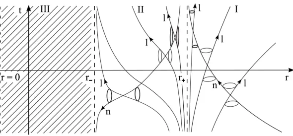
Boyer-Lindquist coordinates are not well-defined at the event horizon atr=r+ (as well as at the Cauchy horizon atr=r−). Light cones of observers approaching the event horizon from outside the black hole close up and become degenerate (see FIG. 1). Moreover, space and time reverse their roles inside the black hole. This makes a direct study of the propagation of Dirac waves across the event horizon impossible in these coordinates. In order to have a consistent description of Dirac waves in the black hole exterior and interior that resolves this problem, advanced Eddington-Finkelstein-type coordinates (AEFTC) are used (see [14, 15] for the original Eddington-Finkelstein null coordinates). This analytically extended coordinate system covers the complete black hole region of the Kruskal manifold and allows for a smooth, well-defined transition across the event horizon. It possesses a proper coordinate time unlike in the case of the original advanced Eddington-Finkelstein null coordinates, which is relevant for a Hamiltonian formulation of the Dirac equation. The AEFTC are constructed as follows. By means of the tangent vectors (10), one can derive two relations between the time and radial coordinates along the principal null geodesics of Kerr geometry given by

dt

dr =±r²+a²

∆ ⇒ t=±

Z r²+a²

∆ dr+c_±=±r_?+c_±, where

r?=r+ r₊² +a²

r+−r₋ ln|r−r+| − r₋² +a²

r+−r₋ ln|r−r₋|

is the so-called Regge-Wheeler coordinate andc_± are constants of integration. These relations motivate the trans- formation

R×R>0×[0, π]×[0,2π)→R×R>0×[0, π]×[0,2π), (t, r, θ, ϕ)7→(τ, r, θ, φ) with orthonormal coordinates adapted to ingoing null geodesics

τ=t+r_?−r=t+ r²₊+a² r+−r−

ln|r−r₊| − r²₋+a² r+−r−

ln|r−r₋| φ=ϕ+

Z a

∆dr=ϕ+ a r+−r₋ ln

r−r+

r−r₋ . This yields the two relations between the new time and radial coordinates

dτ

dr =−1 and dτ

dr = 1 +4M r

∆ .

In the AEFTC system, the event horizon is located at a finite value of the radial coordinate, ingoing light rays are represented by straight lines, and the causal structure is such that the light cones are not degenerate at the event horizon (see FIG. 2). Instead, approaching the event horizon, the light cones tip over until their future light cones are aligned with the horizon, indicating the trapping property of event horizons. The metric (9) represented in these coordinates becomes

g=

1−2M r Σ

dτ⊗dτ−2M r Σ

dr−asin²(θ)dφ

⊗dτ+ dτ⊗

dr−asin²(θ)dφ

−

1 +2M r Σ

dr−asin²(θ)dφ

⊗ dr−asin²(θ)dφ

−Σ dθ⊗dθ−Σ sin²(θ)dφ⊗dφ.

(15)

The associated dual metric tensor reads g= 1

Σ

Σ + 2M r

∂τ⊗∂τ−2M r ∂τ⊗∂r+∂r⊗∂τ

−∆∂r⊗∂r−a ∂r⊗∂φ+∂φ⊗∂r

−∂_θ⊗∂_θ−csc²(θ)∂_φ⊗∂_φ .

r r

r r = 0

II I

-

t

r r = 0

III

- l n

l

l l

l

n l

FIG. 1: Causal structure of Kerr geometry in Boyer-Lindquist coordinates. A projection onto the (t, r)-plane is presented, where every point is a 2-sphere. The real Newman-Penrose null vectorslandn, pointing along the principal null directions of Kerr geometry, form the light cones. The light cones of an observer approaching the event horizon from outside the black hole (r&r+) close up and become degenerate at the event horizon atr=r+. In contrast, they open up when the observer approaches the event horizon from inside the black hole (r %r+). This stems from the fact that the roles of space and time are reversed in the black hole interior. Whenr→ ∞, the light cones become 45^◦-Minkowski light cones because the spacetime is asymptotically flat. In order to avoid the ring singularity, the focus is on regions I and II.

r r r

r = 0

II I III

-

τ

n l

l

l

l

FIG. 2: Causal structure of Kerr geometry in advanced Eddington-Finkelstein-type coordinates. A projection onto the (τ, r)-plane is presented, where every point is a 2-sphere. The real Newman-Penrose null vectors land n, pointing along the principal null directions of Kerr geometry, form the light cones. Ingoing light rays are straight lines pointing in the n-direction. The light cones of an observer approaching the event horizon atr=r+ from outside the black hole (r&r+) tip over until at the event horizon the future light cone is, except from the part that overlaps with the horizon, completely in the black hole interior. This shows the trapping characteristic of the event horizon. Whenr→ ∞, the light cones become 45^◦-Minkowski light cones because the spacetime is asymptotically flat. In order to avoid the ring singularity, the focus is again on regions I and II.

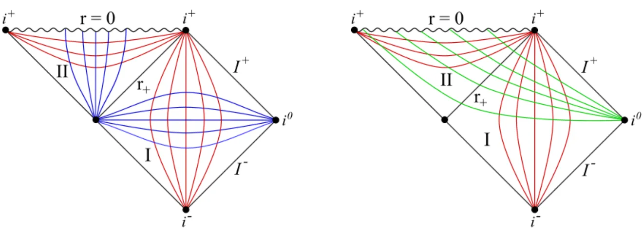
Considering the induced metric on constant-τ hypersurfaces by restricting the metric (15) directly reveals that the constant-τhypersurfaces are space-like and thatτ is a proper coordinate time. In the conformal diagrams shown in FIG. 3 and FIG. 4, the behaviors of the constant-tand constant-rhypersurfaces in Boyer-Lindquist coordinates and of the constant-τ and constant-rhypersurfaces in AEFTC for Schwarzschild and Kerr geometries are schematically depicted. While the Boyer-Lindquist constant-t hypersurfaces become time-like inside the black hole in region II, the AEFTC constant-τ hypersurfaces are always space-like and are smoothly continued through the event horizon at r=r₊. The Carter tetrad (13) and its dual (14) in AEFTC read

l= 1

p2Σ|∆| [∆ + 4M r]∂τ+ ∆∂r+ 2a∂φ

n= r|∆|

2Σ ∂_τ−∂_r

m= 1

√2Σ iasin (θ)∂τ+∂θ+ i csc (θ)∂φ

m=− 1

√

2Σ iasin (θ)∂_τ−∂_θ+ i csc (θ)∂_φ and

l= r|∆|

2Σ sign(∆) dτ+

1−2Σ

∆

dr−asin²(θ)dφ

!

n= r|∆|

2Σ dτ+ dr−asin²(θ)dφ

m= 1

√2Σ

iasin (θ)[dτ+ dr]−Σdθ−i

r²+a²

sin (θ)dφ

m=− 1

√ 2Σ

iasin (θ)[dτ+ dr] + Σdθ−i

r²+a²

sin (θ)dφ .

(16)

Substituting the dual Carter tetrad (16) into the first Maurer-Cartan equation in the Newman-Penrose formalism Eqs.(4), one obtains the spin coefficients for Kerr geometry described by a Carter tetrad in AEFTC

κ=σ=λ=ν= 0, α=−β =− 1 (2Σ)^3/2

r²+a²

cot (θ)−irasin (θ)

π=−τ = iasin (θ)

√

2Σ r−iacos (θ), µ= sign(∆)%=− r|∆|

2Σ

1 r−iacos (θ)

= sign(∆)γ= 1 p|∆|(2Σ)^3/2

M

r²−a²cos²(θ)

−ra²sin²(θ)−iacos (θ)∆

.

i

+

-

0

i

+

i i

I

I - r

r = 0 II

I

i

+

-

0

i

+

i

i r = 0

II I r

I

I -

FIG. 3: Conformal diagrams for Schwarzschild geometry witha= 0 in Boyer-Lindquist coordinates (left) and in advanced Eddington-Finkelstein-type coordinates (right). The blue lines represent constant-thypersurfaces, the red lines constant-r hypersurfaces, and the green lines constant-τ hypersurfaces. The constant-tand constant-rhypersurfaces are restricted to either the black hole exterior or to the black hole interior. Their characters change going from the exterior to the interior, i.e., space-like hypersurfaces become time-like and vice versa. There is no transition across the event horizon. The constant-τ hypersurfaces are space-like outside and inside the black hole, smooth across the event horizon, and end in the curvature singularity atr= 0. The bifurcation 2-sphere is avoided.

i

+

-

0

i i

I II

r = 0

i

III

r

r -

I

I - r -

r

r

i

+

-

0

i i

I II i

r = 0

III

I

I - r -

r -

r

r

r

FIG. 4: Conformal diagrams for Kerr geometry with M² > a² in Boyer-Lindquist coordinates (left) and in advanced Eddington-Finkelstein-type coordinates (right). The blue lines represent constant-thypersurfaces, the red lines constant-r hypersurfaces, and the green lines constant-τ hypersurfaces. As in the Schwarzschild geometry, the constant-thypersurfaces and the constant-rhypersurfaces are restricted to either the black hole exterior or to the black hole interior, changing their characters going from the exterior to the interior without a transition across the event horizon. The constant-τhypersurfaces (cut-off at the Cauchy horizon atr=r−in order to avoid the ring singularity region) are space-like outside and inside the black hole, smooth across the event horizon, and circumvent the bifurcation 2-sphere.

Since the real Newman-Penrose vector lin (16) and, therefore, the spin coefficientsandγ are not well-defined at the event horizon, a renormalization in terms of a type III local Lorentz transformation with the parameters

ξ= p|∆|

r+

and ψ= 0 is applied, leading to a well-defined Carter tetrad

l= 1

√2Σr₊ [∆ + 4M r]∂τ+ ∆∂r+ 2a∂φ

n= r+

√2Σ ∂τ−∂r

m= 1

√

2Σ iasin (θ)∂_τ+∂_θ+ i csc (θ)∂_φ

m=− 1

√2Σ iasin (θ)∂τ−∂θ+ i csc (θ)∂φ

(17)

and dual representation

l= ∆

√2Σr₊ dτ+

1−2Σ

∆

dr−asin²(θ)dφ

!

n= r+

√

2Σ dτ+ dr−asin²(θ)dφ

m= 1

√2Σ

iasin (θ)[dτ+ dr]−Σdθ−i

r²+a²

sin (θ)dφ

m=− 1

√ 2Σ

iasin (θ)[dτ+ dr] + Σdθ−i

r²+a²

sin (θ)dφ .

The corresponding spin coefficients are also finite at the event horizon, yielding κ=σ=λ=ν= 0, α=−β=− 1

(2Σ)^3/2

r²+a²

cot (θ)−irasin (θ)

π=−τ= iasin (θ)

√2Σ r−iacos (θ), µ=− r+

√2Σ r−iacos (θ), %=− ∆

√2Σr+ r−iacos (θ)

γ=− r₊

2^3/2√

Σ r−iacos (θ), =r²−a²−2iacos (θ)(r−M) 2^3/2√

Σr+ r−iacos (θ) .

(18)

In this specific symmetric, renormalized frame represented in AEFTC, the Dirac equation is, as shown in the next section, separable.

IV. THE DIRAC EQUATION IN THE EXTENDED KERR BLACK HOLE SPACETIME

A. Mode Ansatz and Separability

Substituting the renormalized Carter tetrad (17) and the spin coefficients (18) into the Dirac equation in the Newman-Penrose formalism (8), and employing a separation ansatz, which is adapted to the stationarity and axial symmetry of Kerr geometry, intoτ- andφ-modes following the techniques used in Chandrasekhar’s mode analysis (see, e.g., [8])

Fi(τ, r, θ, φ) = exp i(ωτ +kφ)

pr−iacos (θ) Hi(r, θ) and Gi(τ, r, θ, φ) =exp i(ωτ+kφ)

pr+ iacos (θ) Ji(r, θ) (19) with the frequency ω ∈ R, k ∈Z+ 1/2, andi∈ {1,2}, one obtains the coupled, linear, homogeneous first-order PDE system

1

r₊ ∆∂r+r−M+ iω(∆ + 4M r) + 2iakH1+ ∂θ+¹₂cot (θ) +aωsin (θ) +kcsc (θ)H2

=√

2iµ? r−iacos (θ) J1

r₊ ∂_r−iω

H2− ∂_θ+¹₂cot (θ)−aωsin (θ)−kcsc (θ)

H1=−√

2iµ_? r−iacos (θ) J2

1

r₊ ∆∂_r+r−M+ iω(∆ + 4M r) + 2iakJ2− ∂_θ+¹₂cot (θ)−aωsin (θ)−kcsc (θ)J1

=√

2iµ? r+ iacos (θ) H2

r+ ∂r−iω

J1+ ∂θ+¹₂cot (θ) +aωsin (θ) +kcsc (θ)

J2=−√

2iµ? r+ iacos (θ) H1.

(20)

The particularτ- andφ-dependences in the class of mode solutions given by (19) describe perturbations of the black hole background geometry in form of plane waves propagating along the directions of the translation isometries∂_τ and ∂φ of Kerr geometry in AEFTC. Along these directions, the plane wave forms are preserved. The system of Dirac PDEs (20) is separable by means of the product ansatz

H1(r, θ) =R+(r)T+(θ) H2(r, θ) =R−(r)T−(θ) J1(r, θ) =R−(r)T+(θ) J2(r, θ) =R+(r)T−(θ).

(21)

Note that the separability of the Dirac equation depends on the specific choice of the underlying coordinate systems of the fibers of the tangent bundle and of the form of the local tetrad frame. Hence, it is a peculiarity of the Carter tetrad in AEFTC (17) and the corresponding spin coefficients (18) that (20) can be separated via the ansatz (21).

Applying (21) to (20) yields the quadruple of coupled radial equations written in compact form

∆∂r+r−M + iω(∆ + 4M r) + 2iak

R+ =r+ ξ1/3+√ 2iµ?r

R−

r₊ ∂_r−iω

R−= ξ_2/4−√ 2iµ_?r

R+

(22)

and the quadruple of coupled angular equations

∂_θ+¹₂cot (θ) +aωsin (θ) +kcsc (θ)T−=− ξ_1/4−√

2µ_?acos (θ)T+

∂θ+¹₂cot (θ)−aωsin (θ)−kcsc (θ)T+= ξ_2/3+√

2µ?acos (θ)T−,

(23)

where ξi, i∈ {1,2,3,4}, are constants of separation. From the radial equations, it can be directly seen that the identifications ξ1=ξ3 andξ2=ξ4 have to hold, while from the angular equations, one obtains the identifications ξ1=ξ4 andξ2=ξ3. Thus, definingξ:=ξ1=ξ2=ξ3=ξ4, the systems of radial and angular equations (22) and (23) reduce to

∆∂r+r−M + iω(∆ + 4M r) + 2iakR+=r+ ξ+√

2iµ?rR−

r+ ∂r−iω

R−= ξ−√ 2iµ?r

R+

(24)

and

∂_θ+¹₂cot (θ) +aωsin (θ) +kcsc (θ)T−=− ξ−√

2µ_?acos (θ)T+

∂θ+¹₂cot (θ)−aωsin (θ)−kcsc (θ)T+= ξ+√

2µ?acos (θ)T−,

(25)

respectively. The system of radial ODEs (24) can be brought into a more symmetric form by means of the functions Re+=p

|∆|R+ andRe−=r+R−, resulting in the equations

∆∂r+ iω(∆ + 4M r) + 2iak

Re+=p

|∆| ξ+√ 2iµ?r

Re−

∆ ∂r−iω

Re−= sign(∆)p

|∆| ξ−√ 2iµ?r

Re+.

(26)

In a matrix representation, whereRe= Re+,Re−

T

and the partialr-derivative is expressed in terms of the Regge- Wheeler coordinate ∂r= (r²+a²)∆⁻¹∂r_?, these equations become

"

∂r_?+ i r²+a²

ω(∆ + 4M r) + 2ak 0

0 −ω∆

!#

Re= p|∆|

r²+a²

0 ξ+√

2iµ?r sign(∆) ξ−√

2iµ?r 0

!

Re. (27) This representation is advantageous for the subsequent study of the radial asymptotics which is required for a description of the scattering process of Dirac waves by the gravitational field of a black hole or for the construction of an integral representation of the Dirac propagator. Note that in the examination of the asymptoticsr→ ∞and r→r+, the signum function sign(∆) = 1 and forr→r−, sign(∆) =−1. A matrix representation of the angular equations (25), withT = (T+,T−)^T, is given by

√2µ?acos (θ) − ∂θ+¹₂cot (θ) +aωsin (θ) +kcsc(θ)

∂θ+¹₂cot (θ)−aωsin (θ)−kcsc(θ) −√

2µ?acos (θ)

!

T =ξT. (28)

B. Asymptotic Analysis of Radial Solutions at Infinity

In this subsection, following the approach of [18], asymptotic solutions of the radial ODE system (27) forr→ ∞ (r? → ∞) are derived and decay properties of these solutions are examined, showing the control of the error.

Rewriting (27) in the form

∂r_?Re=T(r)Re, (29)

where

T(r) := 1 r²+a²

−i ω(∆ + 4M r) + 2ak p

|∆| ξ+√ 2iµ_?r sign(∆)p

|∆| ξ−√ 2iµ_?r

iω∆

!

, (30)

one can find asymptotic solutions at infinity by first diagonalizing the matrix T by means of the invertible matrix D,D⁻¹T D=S, whereS = diag(λ1, λ2) is the diagonal matrix corresponding toT andλ1/2are the eigenvalues of T. Note that in this limit, ∆>0 and sign(∆) = 1. In terms of the diagonal matrixS, Eq.(29) becomes

∂r_? D⁻¹Re

=

S−D⁻¹(∂r_?D)

D⁻¹Re .

Then, using the ansatz

Re(r_?) =D(r_?) exp iφ−(r?) f1(r?) exp −iφ+(r_?)

f2(r_?)

! ,

one obtains a linear, homogeneous, first-order ODE system for f= (f₁,f₂)^T

∂_r?f=h

S−W⁻¹D⁻¹(∂_r?D)W −i diag ∂_r?φ₋,−∂r?φ₊i f withW := diag exp (iφ−),exp (−iφ+)

. The functionsφ±are fixed by demanding thatS= i diag ∂r_?φ−,−∂r_?φ+

, i.e., ∂r_?φ−=−iλ1and∂r_?φ+= iλ2, yielding

∂r_?f=−W⁻¹D⁻¹(∂r_?D)Wf. (31)

Lemma IV.1. Every nontrivial solutionReof (29) is asymptotically as r→ ∞(r_?→ ∞)of the form

Re(r_?) =Re∞(r_?) +E_∞(r_?) =D_∞ exp iφ₋(r_?) f⁽¹⁾∞

exp −iφ+(r_?) f⁽²⁾_∞

!

+E_∞(r_?) (32)

with the asymptotic diagonalization matrix

D_∞:=































cosh (Ω) sinh (Ω) sinh (Ω) cosh (Ω)



 for ω²≥2µ²_?

√1 2





cosh (Ω) + i sinh (Ω) sinh (Ω) + i cosh (Ω) sinh (Ω) + i cosh (Ω) cosh (Ω) + i sinh (Ω)



 for ω²<2µ²_?,

(33)

where

Ω :=

















 1

4 ln ω+√ 2µ_? ω−√

2µ_?

!

for ω²≥2µ²_?

1 4 ln

√2µ?+ω

√2µ?−ω

!

for ω²<2µ²_?,

(34)

the asymptotic phases

φ_∓(r_?)'



















−p

ω²−2µ²_? r?−2M ±ω+ µ²_? pω²−2µ²_?

!

ln (r?) for ω²≥2µ²_?

p2µ²_?−ω² ir_?−2M ±ω+ iµ²_? p2µ²_?−ω²

!

ln (r_?) for ω²<2µ²_?,

(35)

and the error

||E_∞(r_?)||=

eR(r_?)−Re∞(r_?) ≤ a

r?

(36) for a suitable constant a∈R>0. The asymptotics of the function ffor larger(cf. Eq.(31)) is given by

f_∞= f⁽¹⁾_∞,f⁽²⁾_∞^T

= const.

with an error

||E_f(r_?)||=||f(r_?)−f_∞|| ≤ b r?

for a suitable constant b∈R>0.

Proof. The matrixT defined in (30) converges forr→ ∞ to the matrix T_∞:= lim

r→∞T = i −ω √

2µ?

−√

2µ? ω

! .

Further, it has a regular expansion in powers of 1/r and, thus, in powers of 1/r_?, i.e., T =T_∞+O(1/r_?). The eigenvalues of T_∞ read

λ1/2'







±ip

ω²−2µ²_?∈C for ω²≥2µ²_?

±p

2µ²_?−ω²∈R for ω²<2µ²_?.

The transformation matrixD_∞, which diagonalizesT_∞, is given by (33) with arguments (34). This can be easily shown by direct calculation. SinceT has a regular expansion in powers of 1/r?, both the diagonal matrixS and the transformation matrixDalso have regular expansions in powers of 1/r?. Therefore, with the asymptotic eigenvalues of the matrix T up to first order in 1/r_?

λ_1/2'



















∓ip

ω²−2µ²_?−2iM r?

ω± µ²_? pω²−2µ²_?

!

for ω²≥2µ²_?

∓p

2µ²_?−ω²−2M

r_? iω∓ µ²_? p2µ²_?−ω²

!

for ω²<2µ²_?,

one solves the ODEs for the asymptotic phases stated above Eq.(31) by integration, and immediately obtains (35). With the upper bounds of the Hilbert-Schmidt norms of the inverse and of the partial r?-derivative of the transformation matrix D forr? sufficiently close to infinity

||D⁻¹||_HS≤c and ||∂_r?D||_HS≤ d r²_?,

where candddenote positive constants, one can estimate theC²-norm of Eq.(31)

||∂r_?f|| ≤2||D⁻¹||HS· ||∂r_?D||HS· ||f|| ≤ 2cd

r_?² ||f|| (37)

with ||W||HS =||W⁻¹||HS =√

2. Using the triangle and Cauchy-Schwarz inequalities, it can be shown that the following inequality holds

∂r_?||f||

= |∂r_?hf,fi|

2||f|| = |hf, ∂r_?fi+h∂r_?f,fi|

2||f|| ≤ |hf, ∂r_?fi|+|h∂r_?f,fi|

2||f|| =|hf, ∂r_?fi|

||f|| ≤||f|| · ||∂r_?f||

||f|| =||∂r_?f|| (38)

and, consequently,

∂r_?||f||

≤ 2cd

r²_? ||f||. (39)

Note that||f|| 6= 0 becauseRehas to be nontrivial. Integrating (39) over the Regge-Wheeler coordinate fromr0to r? and applying the triangle inequality for integrals gives

Z r_? r0

∂r_?⁰ ln||f||dr⁰_?

≤ Z r_?

r0

∂r⁰_?ln||f||

dr_?⁰ ≤2cd Z r_?

r0

dr_?⁰

r_?⁰² (40)

for all 0< r₀≤r_?and, hence,

ln||f||

r_? r₀

≤ −2cd r_?⁰

r?

r0

. (41)

Since 0<2cd/r⁰_?

r₀

r_?<∞for all 0< r₀≤r_?<∞, there exists a constantN >0 such that 1

N ≤ ||f|| ≤N (42)

holds. Substituting this into (37), one finds for sufficiently large r?

||∂r_?f|| ≤ b

r²_? (43)

withb:= 2cdN, implying thatfis integrable and has according to (42) a finite, non-zero limitf∞:= limr_?→∞f(r?)6=

0 at infinity. Integrating (43) from r? to ∞and again using the triangle inequality for integrals, one obtains the error estimate

||Ef||=||f−f∞||=

Z ∞ r_?

∂r⁰_?fdr_?⁰

≤ Z ∞

r_?

||∂r⁰_?f||dr⁰_?≤ b r?

. (44)

The 1/r?-decay of the errorE_∞(cf. (36)) follows directly from the substitution of (44) into theC²-norm ofE_∞in (32). Note that the error ED=D−D∞ in (32) is absorbed into the errorE∞.

C. Asymptotic Analysis of Radial Solutions at the Event Horizon

Using the solution ansatz

Re=





 exp

−2ih

ω+kΩ⁽⁺⁾_Kerri r_?

g₁(r_?) g2(r?)







in Eq.(29), where Ω⁽⁺⁾_Kerr:=a/(2M r₊) is the angular velocity of the event horizon of a Kerr black hole, yields an ODE system for the vector-valued functiong= (g1,g2)^T

∂_r?g= i r²+a²







 2k

2MΩ⁽⁺⁾_Kerrr−a 1 0 0 0

! +√

∆

×













√

∆

ω+ 2kΩ⁽⁺⁾_Kerr

exp

2ih

ω+kΩ⁽⁺⁾_Kerri r?

√

2µ?r−iξ

−exp

−2ih

ω+kΩ⁽⁺⁾_Kerri r?

√

2µ?r+ iξ √

∆ω























 g.

(45)

Approaching the event horizon r → r+ (r? → −∞), the right-hand side vanishes and, thus, one obtains the asymptotic solution gr₊:= limr→r₊g= const.

Lemma IV.2. Every nontrivial solutionReof (29) is asymptotically as r→r+ (r?→ −∞)of the form

Re(r?) =Rer₊(r?) +Er₊(r?) =





 exp

−2ih

ω+kΩ⁽⁺⁾_Kerri r?

g⁽¹⁾r+

g⁽²⁾r+





+Er₊(r?) (46) with

g_r+= g⁽¹⁾_r

+,g⁽²⁾_r

+

^T

= const.6= 0 and error with exponential decay

||Er₊(r?)|| ≤pexp (qr?) (47)

forr sufficiently close tor+ and suitable constantsp, q∈R>0. Proof. From Eq.(45), it follows that

∂_r?g=O p

r−r₊

g=O exp (qr_?) g, where r'r₊+ exp (2qr_?) andq:= (r₊−r₋)/ 2(r²₊+a²)

∈R>0. Thus, it exists a constantp⁰∈R>0 such that

||∂r_?g|| ≤p⁰exp (qr?)||g|| (48)

holds for r? sufficiently close to −∞. Similar to the steps (38)-(44) of the previous subsection, one can show that ||g|| is bounded and the error ||g−gr₊|| of the asymptotic solutiongr₊ = const. 6= 0 decays exponentially.

Accordingly, by means of (48), one finds

ln||g||

r₀ r_?

≤ p⁰

q exp (qr⁰_?)

r0

r?

for allr_?≤r₀ and because 0<exp (qr_?⁰)|^r_r⁰

?<∞for all−∞< r_?≤r₀<∞, there is a constantN⁰ >0 such that the norm||g||is bounded

1

N⁰ ≤ ||g|| ≤N⁰. (49)

Substituting (49) into (48) yields

||∂r_?g|| ≤pexp (qr?), (50)

where p:=p⁰N⁰, implying that gis integrable and has a finite, non-zero limit for r? → −∞. Again integrating (50) from−∞tor₀ and applying the triangle inequality for integrals, one obtains

||E_g||=||g−g_r+||=

Z r?

−∞

∂_r⁰

?gdr⁰_?

≤ Z r?

−∞

||∂_r⁰

?g||dr_?⁰ ≤pexp (qr_?), (51) proving the exponential decay of the errorEgof the asymptotic functiongr₊and, therefore, its control forr?→ −∞.

Subsequently, the exponential decay of the error Er₊ (cf. (47)) follows by using (51) in the C²-norm of Er₊ in

(46).