Universit¨ at Regensburg Mathematik
Self-adjointness of the Dirac
Hamiltonian for a class of non-uniformly elliptic boundary value problems
Felix Finster and Christian R¨ oken
Preprint Nr. 18/2015
FOR A CLASS OF NON-UNIFORMLY ELLIPTIC BOUNDARY VALUE PROBLEMS
FELIX FINSTER AND CHRISTIAN R ¨OKEN DECEMBER 2015
Abstract. We consider a boundary value problem for the Dirac equation in a four- dimensional, smooth, asymptotically flat Lorentzian manifold admitting a Killing field which is timelike near and tangential to the boundary. A self-adjoint extension of the Dirac Hamiltonian is constructed. Our results also apply to the situation that the space-time includes horizons, where the Hamiltonian fails to be elliptic.
Contents
1. Introduction 1
2. A Double Boundary Value Problem 6
3. Solution of the Cauchy Problem 11
4. Self-Adjointness of the Dirac Hamiltonian 13
References 13
1. Introduction
Let (M, g) be a four-dimensional, smooth, asymptotically flat Lorentzian manifold with boundary ∂M. We assume that there is a Killing field K which is tangential to and timelike on ∂M. Moreover, we assume that the integral curves of K, defined by the differential equation
˙
γ(t) =K γ(t) ,
exist for all t ∈ R. We also assume that there exists a spacelike hypersurface N with compact boundary ∂N, having the property that every such integral curve γ intersectsN exactly once. This implies thatMand its boundary∂Mhave the product structures
M=R×N and ∂M=R×∂N. (1.1)
Note that our assumptions also imply that the metric g is smooth up to the bound- ary ∂M, thus inducing on∂N a two-dimensional Riemannian metric.
For clarity, we now mention two well-known special cases. If ∂N is empty and N is complete, the product structure (1.1) implies that (M, g) is globally hyperbolic.
Moreover, ifK is timelike in the asymptotic end, the manifold isstationary. However, we point out that we merely assume that K is timelike on the boundary ∂M, but it does not need to be timelike everywhere.
Supported by the DFG research grant “Dirac Waves in the Kerr Geometry: Integral Representa- tions, Mass Oscillation Property and the Hawking Effect.”
1
arXiv:1512.00761v1 [math-ph] 1 Dec 2015
In order to get a better geometric understanding of the above setting, we now con- struct a convenient coordinate system. Choosing the parametrization of each curveγ such that γ(0)∈N, we obtain a global coordinate functionT defined by
T : M→R with T γ(t)
=t . (1.2)
The level sets of this time function give rise to a foliation Nt := T−1(t) by spacelike hypersurfaces with N0 =N. Moreover, the integral curves give rise to isometries
Φt : N→Nt, Φt γ(0)
=γ(t).
Choosing coordinates x on N, the mapping x◦Φ−1t gives coordinates on Nt. Com- plementing this coordinate system by the functiont=T, we obtain coordinates (t, x) with t∈Rand x∈N such that K=∂t. In these coordinates, the line element takes the form
ds2 =gij dxidxj =a(x)dt2+bα(x)dt dxα− gN(x)
αβ dxαdxβ,
whereaandbαare smooth functions, andgN is the induced Riemannian metric onN.
Here we denote the space-time indices by latin lettersi, j∈ {0,1,2,3}, whereas spatial indices are denoted by greek letters α, β ∈ {1,2,3}. This coordinate system can be understood as describing an observer who is co-moving along the flow lines of the Killing field. We note that in the regions where K is timelike, the function a(x) is positive, and the metric is stationary. This is the case if x is near the boundary∂N. However, away from∂N, the functiona(x) could be negative, in which case the metric is not stationary, and t is not a time coordinate. This situation is illustrated in the following example.
Example 1.1. (Kerr geometry in Eddington-Finkelstein-type coordinates) In the recent paper [12], horizon-penetrating Eddington-Finkelstein-type coordinates
(τ, r, θ, φ) with τ ∈R, r∈R+, θ∈(0, π), φ∈(0,2π)
are introduced in the non-extreme Kerr geometry. In these coordinates, the line ele- ment takes the form
ds2=
1−2M r Σ
dτ2−4M r
Σ dr−asin2θ dφ dτ
−
1 +2M r Σ
dr−asin2θ dφ2
−Σdθ2−Σ sin2θ dφ2,
where Σ = r2+a2cos2θ. Moreover, M and aM denote the mass and the angular momentum of the black hole, respectively. The surfacesr±=M ±√
M2−a2 are the event horizonand theCauchy horizonof the black hole. Note that these coordinates are regular on and across the horizons. The two Killing fields describing the stationarity and axisymmetry of the Kerr geometry are ∂τ and∂φ.
We choose a radiusr0< r− inside the Cauchy horizon and let
M={r > r0}, N ={τ = 0, r > r0} and ∂M={r =r0}.
Direct computation shows that the Killing field ∂τ isnot everywhere timelike on∂M (due to an ergo-like region inside the Cauchy horizon; for details see [7]). But takingK as a suitable linear combination of∂τ and ∂φ,
K =∂τ+b ∂φ
with a real constant b=b(r0)6= 0, it turns out that K is a Killing field which satisfies all the above assumptions. This Killing field is spacelike near spatial infinity. ♦ Next, we shall formulate the Dirac equation. To describe spinors one introduces the spinor bundle SM, a vector bundle with fibers SpM 'C4,p ∈M. Each fiber is endowed with an inner product of signature (2,2), referred to as spin scalar product and denoted by
≺.|.p : SpM×SpM→C. The geometric Dirac operator Dtakes the form
D=iγj∇j, (1.3)
where the Dirac matricesγjare related to the metric by the anti-commutation relations γj, γk = 2gjk 11SpM,
and ∇ is the metric connection on the spinor bundle (for more details see [10]). In order to allow for an external potential (like for example an electromagnetic potential), instead of (1.3) we shall consider the more general Dirac operator
D=iγj∇j +B, (1.4)
where B is a smooth matrix-valued potential which we assume to be symmetric with respect to the spin scalar product, i.e. ≺φ|Bψ=≺Bφ|ψ.
We are interested in solutionsψ of the Dirac equation of mass m
(D −m)ψ= 0, (1.5)
with the Dirac operator according to (1.4). In order to analyze the dynamics of Dirac waves, it is useful to write the Dirac equation in the Hamiltonian form
i∂tψ=Hψ , (1.6)
where H is the Dirac Hamiltonian given by H=− γt−1
iγα∇α+B−m
. (1.7)
Taking the domain of definition
D(H) =C0∞
N◦, SM , where
N◦ =N\∂N denotes the interior of N, this Hamiltonian is indeed symmetric (i.e. formally self-adjoint) with respect to the scalar product
(ψ|φ)N = ˆ
N≺ψ|/νφxdµN(x),
where ν is the future-directed normal on N and dµN is the volume form on (N, gN).
This can be verified with the following computation. Using current conservation to- gether with the fact that the metric coefficients do not depend on the coordinate t, we obtain
0 =∂t ψ(t) φ(t)
N = ( ˙ψ|φ)N+ (ψ|φ)˙ N
= (−iHψ) φ
N + ψ
(−iHφ)
N =i (Hψ|φ)N −(ψ|Hφ)N .
In order to pose the Cauchy problem for the Dirac equation (1.5), one needs to specify initial and boundary conditions. We choose initial data which is smooth and compactly supported,
ψ|N =ψ0 ∈C0∞(N, SM). (1.8)
Moreover, we impose the boundary conditions
(n/−i)ψ|∂M= 0, (1.9)
where the slash denotes Clifford multiplication, and n is the inner normal on ∂M (meaning that for everyp∈∂Mthere is a curvec: [0, δ)→Mwithc(0) =pand ˙c(0) = n(p)). Clearly, the initial data must be compatible with the boundary conditions, meaning that (/n−i)ψ0|∂M= 0. These boundary conditions, which are very similar to those introduced in [5, Section 2], have the effect that Dirac waves are reflected on∂M. They can also be understood in analogy to the chiral boundary conditions in [3, 8]. The difference is that, instead of the intrinsic Dirac operator on the hypersurface, we here consider the Hamiltonian obtained from the Dirac operator in space-time by separating thet-dependence. This gives rise to the additional factor (γt)−1in (1.7). Our boundary conditions (1.9) can be understood as an adaptation of the chiral boundary conditions in [3, 8] to the Hamiltonian (1.7).
The boundary conditions (1.9) must be incorporated in the functional analytic set- ting. To this end, one extends the domain of definition to
D(H) =
ψ∈C0∞(N, SM) with (/n−i)ψ|∂N = 0 . (1.10) Then the operator H is again symmetric, as the following consideration shows. First, we rewrite the scalar product (ψ|Hφ)N in a more convenient form. Applying the relations (γt)2 =gtt11SxM andν/=γt/p
gtt, we obtain /
ν(γt)−1 = 1
gtt /ν γt= 11SxM pgtt . Making use of the form of the Hamiltonian (1.7), this leads to
(ψ|Hφ)N =−i ˆ
N≺ψ|γα∇αφx 1
pgtt dµN(x) + (lower order terms). Now a direct computation of the boundary terms yields
(ψ|Hφ)N−(Hψ|φ)N =i ˆ
∂N≺ψ|/nφx 1
pgtt dµ∂N(x)
(we note that the angular derivatives do not give rise to boundary terms because∂N is compact without boundary). Using the boundary conditions in (1.10), for all x∈∂N we obtain
i≺ψ|φx =≺ψ|nφ/ x=≺nψ|φ/ x =−i≺ψ|φx,
proving that the boundary values indeed vanish. This shows that H is symmetric.
In order to solve the Cauchy problem and to analyze the long-time behavior of its solutions, it is of central importance to construct a self-adjoint extension ofH. Namely, with such a self-adjoint extension at hand, the solution of the Cauchy problem for the Dirac equation (1.5) with initial values (1.8) and boundary conditions (1.9) can be expressed using the spectral theorem for self-adjoint operators as
ψ(t) =e−itH ψ0 = ˆ
σ(H)
e−iωtdEωψ0.
This formula is also the starting point for a detailed analysis of the long-time behavior of ψ using spectral methods, similar as carried out in the exterior region of Kerr geometry in [5, 4]. In the present paper, we succeed in constructing a self-adjoint extension:
Theorem 1.2. The Dirac Hamiltonian (1.7) with domain of definition D(H) =n
ψ∈C0∞(N, SM) with (/n−i) Hpψ
∂N = 0 for allp∈N0
o
(1.11) is essentially self-adjoint.
Note that the domain (1.11) is smaller than (1.10). This is preferable because we want that the Cauchy problem has a global solution inC0∞(N, SM) (see the strategy of our proof as described at the end of this section).
We conclude this section by putting our result into the context of previous work, and explaining the strategy of our proof. The Cauchy problem and the problem of constructing a self-adjoint extension of the Dirac Hamiltonian have been studied in several simpler situations:
(i) IfNis a complete manifold without boundary, the Cauchy problem can be solved using the theory of symmetric hyperbolic systems (see for example [9, 14, 6]). In this construction, one works with local charts with local time functions. Since the resulting local solutions coincide in the regions where the charts overlap, this procedure gives rise to a unique, global smooth solution inM. Then, restricting this solution to the spacelike hypersurfaces of constant t, one obtains a family of time evolution operators
Ut0,t : C∞ {t} ×N, SM
→C∞ {t0} ×N, SM ,
which form a group. This makes it possible to apply [2] to conclude that the Hamiltonian is essentially self-adjoint on C∞(N, SM).
(ii) In the ultrastatic situation
ds2=dt2− gN
αβdxαdxβ, the Hamiltonian can be written as
H=
0 DN DN 0
,
where DN is the intrinsic Dirac operator onN. This makes it possible to apply the results in the Riemannian setting as worked out in detail in [1].
(iii) In the static situation
ds2 =a(x)dt2− gN
αβ dxαdxβ, the Hamiltonian can be written as
H =p a(x)
0 DN DN 0
+ (zero-order terms).
Introducing a suitable scalar product on the Dirac wave functions, this Hamilton- ian is again symmetric, making it possible to again apply the results of [1].
In the situation under consideration here, there is the major complication that the Hamiltonian is in general not uniformly elliptic, so that the methods in [1] no longer apply. In order to explain the problem, we now consider the principal symbol of the Dirac Hamiltonian. According to (1.7), the principal symbol takes the form
P(x, ξ) =−i γt−1
γαξα.
The ellipticity condition states that the principal symbol should be bounded from below by
P(x, ξ)
≥δkξk2
for a suitable constantδ >0 (for basics on the principal symbol and the connection to ellipticity see for example [13, Section 5.11]). In order to verify whether this condition holds, it is most convenient to compute the determinant of the principal symbol.
Namely,
detP(x, ξ) = det (γt)−1
det γαξα , and using that
(γt)−1(γt)−1= 11SxM
gtt , γαξαγβξβ =gαβξαξβ11SxM, we obtain
detP(x, ξ) =
gαβξαξβ gtt
2
.
This computation shows that the Hamiltonian fails to be elliptic if gαβξαξβ = 0 for a non-zero ξ. In the example of the Kerr metric in Eddington-Finkelstein-type coordinates [12], this is the case precisely on the event and Cauchy horizons. More generally, the points where the Hamiltonian fails to be elliptic can be used as the definition of the horizonsof our space-time. Thus we face the major problem that the Hamiltonian is not elliptic on the horizons.
Our strategy to solve this problem is to split up the solution of the Cauchy problem into two separate problems: Near the boundary, we rewrite the problem in a form where the results in [1] apply. Away from the boundary, however, we use the theory of symmetric hyperbolic systems. Making essential use of finite propagation speed, adding the two solutions gives rise to a unique solution of our boundary value problem for small times. By iterating the procedure, we get unique global, smooth solutions, making it possible to proceed as in (i) above by applying [2].
2. A Double Boundary Value Problem
As a technical tool for the proof of Theorem 1.2, we need to show that the Cauchy problem (1.5), (1.8) with boundary conditions (1.9) has global smooth solutions. Our method is to split up the Cauchy problem into two separate problems near and away from the boundary. In preparation, we now introduce additional boundary conditions on a suitable surfaceY near∂M. We work in Gaussian normal coordinates in a tubular neighborhood inN of ∂N. Thus for anyp∈∂N, we letcp(r) for 0≤r < rmax(p) be the geodesic in N with the initial conditions
cp(0) =p and c0p(0) =u ,
whereu∈TpN is the inner normal to∂N. Since∂N is compact, we can choosermax>
0 independent ofp to obtain a mapping
c : [0, rmax)×∂N→N, c(r, p) =cp(r).
Applying the implicit function theorem, possibly by decreasing rmax we can arrange that c is a diffeomorphism. We introduce the sets obtained from∂N by the geodesic flow by
∂N(r) =c(r, ∂N).
Choosing coordinates Ω = (ϑ, ϕ) on∂N gives a corresponding coordinate system (r,Ω) on N. In these coordinates, the metric on N takes the form
(gN)αβ =
1 0 0 g∂N(r)
and thus (gN)αβ =
1 0 0 g∂N(r)−1
. (2.1)
Taking againtas the time coordinate, we obtain a coordinate system (t, r,Ω) witht∈ R,r∈[0, rmax) ofM which describes a neighborhood of∂M.
We now introduce the following new boundary value problem. Let X be the space- time region
X=
(t, r,Ω)
0≤r≤rmax/2 .
This is a Lorentzian manifold whose boundary ∂X consists of ∂M as well as the three-dimensional surface
Y :=
(t, rmax/2,Ω) .
Possibly by decreasingrmax, we can arrange that K is timelike inX, implying that Y is a timelike surface. The inner normal on Y is again denoted byn. We consider the initial value problem
(D −m)ψ= 0 inX , ψ|N =ψ0 ∈C∞(N∩X, SM), (2.2) with the boundary conditions
(/n−i)ψ|∂X = 0, (2.3)
where∂X =∂M∪Y now has two components. It is again useful to rewrite the Dirac equation in the Hamiltonian form (1.6) with the Hamiltonian (1.7). In order to take into account the boundary conditions, we now choose the domain of definition as the Sobolev space
D(H) =
ψ∈W1,2(X∩N, SM)
(/n−i)ψ|∂X∩N = 0 . (2.4) The next proposition gives a spectral decomposition ofH.
Proposition 2.1. There is a countable orthonormal basis (ψn)n∈N, ψn ∈ D(H), of eigenfunctions of H.
Proof. Our method is to apply the abstract spectral theorem given in [1, Theorem 4.1].
The task is to verify the spectral conditions (C0)–(C4), which in our setting are stated as follows:
(C0) H : D(H)→L2(X) is linear and bounded in the W1,2-topology onD(H).
(C1) The G˚arding inequality holds: There exists a constant C such that for all ψ ∈ D(H),
kψk2W1,2(X∩N)≤C ˆ
X∩N
(≺Hψ|/νHψx+≺ψ|νψ/ x)dµN(x). (2.5) (C2) Weak solutions are strong solutions (“elliptic regularity”): If φ ∈ L2(X ∩N)
satisfies ˆ
X∩N
≺Hψ|/νφxdµN(x) = 0 for all ψ∈D(H), thenφ∈D(H).
(C3) H is symmetric, i.e. for allψ, φ∈D(H), ˆ
X∩N
≺ψ|νHφ/ xdµN(x) = ˆ
X∩N
≺Hψ|νφ/ xdµN(x). (C4) D(H) is dense inL2(X∩N).
The validity of condition (C0) follows immediately from the fact thatHis a differential operator of first order. The symmetry property (C3) was verified after (1.10). The denseness property (C4) is obvious. In order to verify the G˚arding inequality (C1), we exploit the specific form of the Hamiltonian (1.7). The contribution to≺Hψ|/νHψx involving first derivatives squared is estimated by
≺(γt)−1γα∇αψ|/ν(γt)−1γβ∇βψx≥c gNαβk∇αψk k∇βψk
(for a suitable constantc >0), where we used that the inner product≺.|ν./ is positive definite and that the matrices (γt)−1andγαare uniformly bounded onX. Introducing the notation k∇ψk2 =gNαβk∇αψk k∇βψkand estimating the coefficients of the lower order terms by suitable constants d1, d2 >0, we obtain the estimate
≺Hψ|νHψ/ x ≥ck∇ψk2−d1k∇ψk kψk −d2kψk2
≥ c
2 k∇ψk2− d21
2c +d2
kψk2. Hence
kψk2W1,2(X∩N)= ˆ
X∩N
k∇ψk2+kψk2
dµN(x)
≤ ˆ
X∩N
2
c ≺Hψ|/νHψx+2 c
d21 2c +d2
kψk2+kψk2
dµN(x). This shows that condition (C1) holds.
It remains to derive the regularity condition (C2). This consists of two parts: the interior regularity and the regularity at the boundary. For the interior regularity, we need to show that the operatorH is uniformly elliptic (see [1, Theorem 3.7]). To this end, we make use of the fact that the Killing fieldKis timelike inX. As a consequence, we can use it to define a norm on the spinors by
kψ(x)k2x :=≺ψ|γtKγ/ tψx. Using this norm, we have
ξα (γt)−1γα ψ)(x)
2
x=ξαξβ ≺(γt)−1γαψ|γtKγ/ t(γt)−1γβψx
=ξαξβ ≺γαψ|Kγ/ βψx.
Since K/ =γt, this matrix anti-commutes with the matricesγβ. Therefore,
ξα (γt)−1γα ψ)(x)
2
x=−ξαξβ ≺γβγαψ|Kψ/ x
=−gαβ ξαξβ ≺ψ|Kψ/ x=−gαβξαξβ
(γt)−1ψ
2 x, showing explicitly that H is uniformly elliptic. To see that the matrix (γt)−1 is uni- formly bounded, we note that, using Cramer’s rule,
(γt)−12
= 11SxM
gtt =−detgαβ
gtt =−detgαβ
hK, Ki , which is indeed bounded because K is timelike in X.
The remaining proof of the boundary regularity is a subtle point, which we now treat in detail. We first note that, by localizing with a test function and using the interior regularity, it suffices to consider weak solutions whose support is in a small neighborhood of ∂N orY ∩N. Since both cases can be treated in the same way, we may assume that the solution vanishes identically outside a small neighborhood of∂N.
Our goal is to apply [1, Theorem 5.11]. Simplifying the statement of this theorem and adapting it to our setting, this theorem gives boundary regularity for boundary value problems of the form
Lu=f (2.6)
P u|∂N = 0. (2.7)
Here P is a projection operator on L2(∂N). Moreover, Lis the differential operator L=∂r+A+B ,
where the operatorsAandBare of the following form. The operatorA:W1,2(∂N)→ L2(∂N) is an angular differential operator which is independent ofrand satisfies again the above spectral conditions (C0)–(C4). The operatorB:W1,2(X∩N)→L2(X∩N), on the other hand, should be such that its first-order terms vanish on∂N.
The first step is to rewrite the Dirac equation and the boundary conditions in the re- quired form. Suppose thatψis a weak solution of the inhomogeneous equationHψ=f satisfying the boundary conditions (2.3). Moreover, assume thatψandf are supported in a small neighborhood of∂N. In order to implement the boundary conditions on∂N, we choose the projection operatorP as
P = 1
2 i/n+ 1 .
Next, using (1.7), one can write the differential equation (2.6) as
∂r+ (γr)−1 γϑ∂ϑ+γϕ∂ϕ
+E
ψ=i(γr)−1γtf ,
where ϑand ϕare coordinates on∂N, and E is a zero-order operator. We choose A= (γr)−1 γϑ∂ϑ+γϕ∂ϕ
∂N+Z (2.8)
B = (γr)−1 γϑ∂ϑ+γϕ∂ϕ
+E−A , (2.9)
where Z is a zero-order operator on ∂N to be determined below.
The crucial point is to show that by a suitable choice of the scalar product and the zero-order operator Z, we can arrange that the operator A is symmetric. We choose the scalar product as
h.|.i∂N = ˆ
N
≺.|K ./ xdµ∂N (2.10) (since K is timelike near ∂N, this inner product is indeed positive definite). Using the form of the metric (2.1) in our Gaussian normal coordinate system, the following anti-commutation relations hold,
{K, γ/ r}= 2gtr = 2δtr= 0 {K, γ/ ϑ}={K, γ/ ϕ}= 0 {γr, γϑ}={γr, γϕ}= 0.
As a consequence, the matrices (γr)−1γϑand (γr)−1γϕare anti-symmetric with respect to the scalar product (2.10). Thus, setting
Z =−1
2 A0−A∗0
with A0 := (γr)−1 γϑ∂ϑ+γϕ∂ϕ
∂N,
where the star denotes the formal adjoint with respect to the scalar product (2.10), the operator Z is indeed a multiplication operator. Moreover, using the above formulas
for Z and A0 in (2.8), one sees thatA= (A0+A∗0)/2, which is obviously symmetric.
Finally, it is clear by construction that the restriction of B to∂N is a multiplication operator.
From this construction, it is obvious that the operator A has the above proper- ties (C0), (C3) and (C4). In order to prove the G˚arding inequality (C1) and the elliptic regularity (C2), we make use of the anti-commutation relations
n
(γr)−1γα,(γr)−1γβ o
=− 1 grr
γα, γβ =−2 gαβ
grr forα, β ∈ {ϑ, ϕ}. Hence the operator A2 is of the form
A2= 1
grr ∆S2 + (lower order terms).
This is an elliptic operator on a bounded domain. Standard elliptic theory implies (C1)
and (C2).
The spectral decomposition of Proposition 2.1 implies that the mixed initial/boun- dary value problem (2.2), (2.3) has a unique weak solution inW1,2(X∩N, SM) given by
ψ(t, x) =
∞
X
n=1
cne−iωntψn(x) with cn= ˆ
X∩N
≺ψn|/νψ0ydµN(y), (2.11) where ωn is the eigenvalue of ψn. In order to apply [2], we want a solution which is smooth for all times. We now state the corresponding necessary and sufficient conditions.
Lemma 2.2. Suppose that ψ0 satisfies the conditions (/n−i) Hpψ0
∂N = 0 for allp∈N0. (2.12) Then the solution ψ of the mixed initial/boundary value problem (2.2), (2.3) is in the class Csc∞(M, SM), where the index “sc” denotes solutions of space-like compact support (i.e. suppψ(t, .) is a compact subset of N for all t ∈ R). Conversely, if a solution of the mixed initial/boundary value problem is smooth, then ψ0 satisfies the conditions (2.12).
Proof. Letψ be the solution of the mixed initial/boundary value problem (2.2), (2.3) for ψ0 satisfying (2.12). In order to show thatψ is smooth, it clearly suffices that all time derivatives of ψ exist and are smooth inx. To this end, we consider the partial sums of (2.11)
ψN(t, x) =
N
X
n=1
cne−iωntψn(x) for given N ∈N. Differentiating ptimes with respect tot gives
(i∂t)pψN(t, x) =
N
X
n=1
ωnpcne−iωntψn(x). Furthermore,
ωpncn= ˆ
X∩N≺Hpψn|/νψ0ydµN(y) = ˆ
X∩N≺ψn|/ν Hpψ0
ydµN(y),
where we iteratively integrated by parts and used the boundary conditions (2.12).
Since the function ˜ψ0 := Hpψ0 is again in D(H) given by (2.4), we can take the limitN → ∞ to conclude that
(i∂t)pψ(t, x) =
∞
X
n=1
˜
cne−iωntψn(x) with c˜n= ˆ
X∩N
≺ψn|ν/ψ˜0ydµN(y). This shows that ψ is indeed a smooth solution.
Assume conversely thatψ is a smooth solution to the mixed initial/boundary value problem (2.2), (2.3). Then (/n−i)ψ(t)|∂N = 0 for all t. Differentiating p times with respect tot gives
0 = (i∂t)p
(/n−i)ψ(t)|∂N
t=0 = (/n−i) Hpψ0
∂N ,
proving (2.12).
3. Solution of the Cauchy Problem
We now return to the Cauchy problem (1.5), (1.8) with boundary conditions (1.9).
Thus we seek for solutions of the Dirac equation in the Hamiltonian form
i∂tψ=Hψ inM, (3.1)
with initial and boundary values
ψ|N =ψ0 and (/n−i)ψ|∂M= 0, (3.2) where the initial data is in D(H) as given in (1.11), i.e.
ψ0 ∈n
ψ∈C0∞(N, SM) with (/n−i) Hpψ
∂N = 0 for allp∈N0
o
. (3.3) Lemma 3.1. There isε >0such that the mixed initial/boundary value problem (3.2), (3.3) has a unique solution ψ in the class
ψ∈C0∞([0, ε)×N, SM) with (/n−i) (Hpψ)|[0,ε)×∂N = 0 for all p∈N0 . Proof. Near ∂N, we again choose the Gaussian normal coordinate system where the metric takes the form (2.1). Moreover, we choose εso small that the future develop- ment J∨ of initial data sets has the properties
J∨
(0, r,Ω)
r < rmax/4
∩ {ε} ×N
⊂
(0, r,Ω)
r < rmax/2 (3.4) J∨
(0, r,Ω)
r > rmax/8
∩ {ε} ×N
⊂
(0, r,Ω)
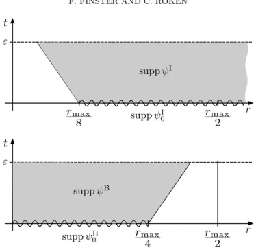
r >0 . (3.5) We next decompose the initial data into a contribution ψ0B near the boundary ∂N and a contribution ψI0 supported in the interior of N,
ψ0 =ψ0B+ψ0I. To this end, we let η∈C0∞ (−rmax/4, rmax/4)
be a test function withη|[0,rmax/8]≡1 and set (see Figure 1)
ψB0 :=η(r)ψ0 and ψI0:=ψ0−ψ0B.
We take ψ0I as initial value problem for the Dirac equation without boundary con- ditions,
i∂tψI=HψI inX , ψI|N =ψI0.
Figure 1. Decomposition of the solution of the Cauchy problem.
Using the theory of symmetric hyperbolic equations (see [9, Section 5.3], [14, Sec- tion 16], [11, Section 7] or [6, Chapter 5]), this initial value problem has a unique solution ψIin the classCsc∞ [0, ε)×N) (just as explained in (i) on page 5). Note that, due to finite propagation speed and (3.5), the solution vanishes identically near ∂M (see the top picture in Figure 1).
Next we take ψ0B as initial values for the double boundary value problem, i.e.
i∂tψB=HψB inX , ψB|N =ψ0B, (/n−i)ψB|∂M= 0. (3.6) According to Lemma 2.2, this mixed initial/boundary value problem has a smooth so- lution which satisfies the initial and boundary conditions in (3.6) pointwise. Moreover, due to finite propagation speed and (3.4), we know that the solutionψB vanishes near the boundary {r =rmax/2}, i.e.
suppψB(t, .)⊂[0, rmax/2)×∂N for all t∈[0, ε)
(see the bottom picture in Figure 1). Therefore, extending ψB by zero, we obtain a global solution in all M.
The function ψ = ψB+ψI is the desired solution of our mixed initial/boundary value problem. Uniqueness follows immediately from standard energy estimates for symmetric hyperbolic systems (see for example [9, Section 5.3]).
Corollary 3.2. The mixed initial/boundary value problem (3.2), (3.3) has a unique global solution ψ in the class of smooth wave functions with spatially compact support satisfying the boundary conditions,
n
ψ∈Csc∞(M, SM) with (/n−i) Hpψ
∂M= 0 for all p∈N0
o .
The resulting time evolution operator is unitary with respect to the scalar product (ψ|φ)N =
ˆ
N≺ψ(t, x)|ν/(t, x)φ(t, x)xdµN(x). (3.7)
Proof. Since the existence time ε in Lemma 3.1 does not depend on the initial data, we can iterate the procedure to obtain smooth solutions for arbitrarily large times.
Moreover, solving backwards in time, one can also obtain smooth solutions for arbi- trarily large negative times. We thus obtain global smooth solutionsψ∈Csc∞(M, SM).
The symmetry of H (as shown after (1.10)) implies that the scalar product (3.7) is preserved under time evolution. Therefore, the time evolution operator is unitary.
4. Self-Adjointness of the Dirac Hamiltonian
We now give the proof of Theorem 1.2. Let H be the Dirac Hamiltonian with do- main D(H) given by (1.11). Corollary 3.2 shows that the time evolution operator for the mixed initial/boundary value problem (3.2), (3.3) defines a one-parameter group acting onD(H). Moreover, it is obvious that the domain is invariant under the action of H. Therefore, we can apply the result by Chernoff [2, Lemma 2.1] to conclude that H is essentially self-adjoint on D(H). This completes the proof of Theorem 1.2.
Acknowledgments: F.F. is grateful to the Center of Mathematical Sciences and Appli- cations at Harvard University for hospitality and support.
References
[1] R.A. Bartnik and P.T. Chru´sciel, Boundary value problems for Dirac-type equations, arXiv:math/0307278 [math.DG], J. Reine Angew. Math.579(2005), 13–73.
[2] P.R. Chernoff,Essential self-adjointness of powers of generators of hyperbolic equations, J. Func- tional Analysis12(1973), 401–414.
[3] A.J. Dougan and L.J. Mason,Quasilocal mass constructions with positive energy, Phys. Rev. Lett.
67(1991), no. 16, 2119–2122.
[4] F. Finster, N. Kamran, J. Smoller, and S.-T. Yau, Decay rates and probability estimates for massive Dirac particles in the Kerr-Newman black hole geometry, arXiv:gr-qc/0107094, Comm.
Math. Phys.230(2002), no. 2, 201–244.
[5] , The long-time dynamics of Dirac particles in the Kerr-Newman black hole geometry, arXiv:gr-qc/0005088, Adv. Theor. Math. Phys.7(2003), no. 1, 25–52.
[6] F. Finster, J. Kleiner, and J.-H. Treude,An Introduction to the Fermionic Projector and Causal Fermion Systems, in preparation.
[7] F. Finster and C. R¨oken,The massive Dirac equation in Kerr geometry in Eddington-Finkelstein- type coordinates: Spectral theory of the Hamiltonian and integral representation of the propagator, in preparation.
[8] G.W. Gibbons, S.W. Hawking, G.T. Horowitz, and M.J. Perry,Positive mass theorems for black holes, Comm. Math. Phys.88(1983), no. 3, 295–308.
[9] F. John, Partial Differential Equations, fourth ed., Applied Mathematical Sciences, vol. 1, Springer-Verlag, New York, 1991.
[10] H.B. Lawson, Jr. and M.-L. Michelsohn,Spin Geometry, Princeton Mathematical Series, vol. 38, Princeton University Press, Princeton, NJ, 1989.
[11] H. Ringstr¨om, The Cauchy Problem in General Relativity, ESI Lectures in Mathematics and Physics, European Mathematical Society (EMS), Z¨urich, 2009.
[12] C. R¨oken, The massive Dirac equation in Kerr geometry: Separability in Eddington-Finkelstein- type coordinates and asymptotics, arXiv:1506.08038 [gr-qc] (2015).
[13] M.E. Taylor,Partial Differential Equations. I, Applied Mathematical Sciences, vol. 115, Springer- Verlag, New York, 1996.
[14] , Partial Differential Equations. III, Applied Mathematical Sciences, vol. 117, Springer- Verlag, New York, 1997.
Fakult¨at f¨ur Mathematik, Universit¨at Regensburg, D-93040 Regensburg, Germany E-mail address: finster@ur.de, Christian.Roeken@mathematik.ur.de