Indirect inference of synergistic and alternative signalling of intracellular pathways
DISSERTATION ZUR ERLANGUNG DES DOKTORGRADES DER NATURWISSENSCHAFTEN (DR. RER. NAT.)
DER FAKULTÄT FÜR BIOLOGIE UND VORKLINISCHE MEDIZIN DER UNIVERSITÄT REGENSBURG
vorgelegt von
Martin Franz-Xaver Pirkl
aus
Neumarkt i.d. Opf
im Jahr 2016
Der Promotionsgesuch wurde eingereicht am:
07.06.2016
Die Arbeit wurde angeleitet von:
Prof. Rainer Spang Unterschrift:
Martin Pirkl
Acknowledgements
I like to thank my supervisor Rainer Spang for making the transition from “pure” mathe- matics (technically applied mathematics, but with paper and pencil instead of a comput- ers) to statistical Bioinformatics as smooth as possible. I would also like to thank my two mentors Michael Boutros from the German Cancer Research Center in Heidelberg and Elmar Lang from the Biophysics department for their cooperation and guidance in RNA interference respectively machine learning. Furthermore, I am very thankful to Michael Boutros’ group for generating the vast amount of data we analyzed in chapter 7. The Microarray Data analysed in chapter 6 was produced by Dieter Kube’s group in Götting and for that I am also very thankful. I want to thank the author of the original Nested Effects Models Florian Markowetz for the invitation to visit his group in Cambridge and Julio Saez-Rodriguez to take the time to introduce me to his group in Hinxton, also.
Last, but not least I thank the whole group (plus alumni) of the department of sta- tistical Bioinformatics at the University of Regensburg for healthy discussions, work and non-work related, especially the Nested Effects Model and Bayesian Networks people. A special high five goes out to the people of the after lunch table football group.
Publications
Parts of chapters 4, 5, 6 and 7 in this Thesis are published or in preparation for publica- tion.
Pirkl, Martin, Hand, Elisabeth, Kube, Dieter, & Spang, Rainer. 2016. Analyzing syner- gistic and non-synergistic interactions in signalling pathways using Boolean Nested Effect Models. Bioinformatics, 32(6), 893900.
Kranz, Dominique, Pirkl, Martin, Leible, Svenja, Kerr, Grainne, Spang, Rainer, &
Boutros, Michael. 2016. Regulatory networks of Tnfα and Trail induced gene regula- tion in hepatocellular carcinoma cell lines and primary hepatocytes. in preparation.
“I don’t think that math is gonna bring you back from the dead.”
– Frylock, Aqua Teen Hunger Force
Contents
Table of contents ix
1 Introduction 1
1.1 Motivation . . . 1
1.2 Organization . . . 3
1.3 Intracellular Signalling Pathways in the Context of Cancer . . . 3
2 Boolean Hyper-Graphs 7 2.1 Boolean Algebra . . . 7
2.2 Graphs and Hyper-Graphs . . . 9
3 Network Models 13 3.1 Bayesian Networks . . . 13
3.2 Nested Effects Models . . . 14
3.2.1 Original approach . . . 15
3.2.2 Optimization . . . 16
3.2.3 Factor Graph Nested Effects Models . . . 18
3.2.4 Dynamic Nested Effects Models . . . 19
3.2.5 Partial Nested Effects Models . . . 23
3.3 CellNet Optimizer . . . 26
3.3.1 Model inference with a genetic algorithm . . . 26
4 Boolean Nested Effects Models 31 4.1 Complex and Alternative signalling . . . 31
4.1.1 Combinatorial signalling . . . 31
4.2 Pathway model and score . . . 32
4.2.1 Signalling Pathways and Deterministic Boolean Networks . . . 32
4.2.2 Experimental design and data . . . 33
4.2.3 Expected and Observed Response Schemes . . . 33
4.2.4 Scoring hyper-graphs . . . 33
4.2.5 Assigning E-genes to S-genes . . . 35
4.2.6 Model adaptive discretization score . . . 35
4.2.7 Marginal Likelihood Formulation . . . 37
4.2.8 Other Similarity Measures . . . 37
4.2.9 Automatic E-gene Selection . . . 38
4.2.10 Local residuals . . . 38
4.3 Optimization . . . 39
4.3.1 Network Equivalence . . . 39
4.3.2 Search Algorithms . . . 47
4.4 Nested Effects Models as restricted Boolean Networks . . . 49
4.5 A Bayesian Networks view on Boolean Networks . . . 51
5 Simulation study 53 5.1 Principle simulations . . . 53
5.1.1 B-NEM accurately estimate the equivalence class of networks with up to 30 S-genes. . . 54
5.1.2 Network reconstruction is sensitive to the strength of the prior knowledge network. . . 54
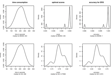
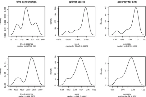
5.2 GA vs BGNS . . . 57
6 The Role of Pi3k and Tak1 in BCR signalling of Burkitt’s Lymphoma Celline BL2 59 6.1 BCR signalling . . . 59
6.2 Gene expression profiling and preprocessing . . . 59
6.3 Results . . . 60
6.3.1 Prior knowledge in BCR signalling . . . 60
6.3.2 Calibrating the sparseness parameter ζ . . . 61
6.3.3 The role of PI3K and TAK1 . . . 61
7 Analyzing Crosstalk of Inflammatory and Apoptotic Signalling in Hep- atocellular Carcinoma 69 7.1 Hepatocellular Carcinoma . . . 69
7.1.1 Tnf-α and Trail signalling in HCC . . . 69
7.2 Data generation and processing . . . 70
7.3 Prior knowledge . . . 73
7.4 Results . . . 74
7.4.1 The core network . . . 74
7.4.2 Testing unknown S-genes for interaction . . . 81
8 Applying B-NEM to time series data 83 8.1 Algorithm . . . 83
8.2 Simulation . . . 84
8.2.1 Data generation . . . 84
8.2.2 Results . . . 85
8.3 Self renewal in embryonic stem cells . . . 86
8.3.1 Resolving Dynamic Feedback . . . 87
9 Conclusion and Outlook 89
A Signal Propagation 91 A.1 Transitivity . . . 91 A.2 Simulated signal propagation . . . 94 A.3 Different Problem - same Method . . . 99
B Similarity Measures 103
C Normalization to [0,1] 106
D Supplementary Figures 108
List of Algorithms 119
List of Figures 124
List of Tables 125
Bibliography 133
Abbreviations 135
Curriculum Vitae 137
1
Introduction
1.1 Motivation
Cells process input signals to output signals using a network of cellular signalling path- ways (Berg et al. (2012)). For example, a small molecule binds a membrane receptor.
The signal is brought into the cell via structural modification of the receptor. A set of kinases and other signalling molecules propagate the signal through the cytosol. This involves both activation and repression of proteins. Often complexes of multiple proteins must form before a signal propagates. Eventually, the signal enters the nucleus and tran- scription factors become activated. Finally, the combination of activated transcription factors and regulatory co-factors leads to the transcription of a large set of genes. Even- tually, this can lead to changes of the cell phenotype. Some of the involved molecules are also part of other pathways linking multiple pathways together. Understanding the structure and the interplay of pathways is crucial both for understanding the cellular mechanism and for designing novel therapies that target specific pathways.
Inferring networks from molecular profiles is a well developed field in bioinformatics.
Transcriptional data can be generated more easily compared to protein activation data.
Consequently, many algorithms were developed that focus on the reconstruction of reg- ulatory networks, for example Gaussian graphical models (GGM) (Schäfer & Strimmer (2005)), Bayesian networks (Friedman et al. (2000)) or the PC-algorithm (Kalisch &
Bühlmann (2007)), the Algorithm for the Reconstruction of Accurate Cellular Networks (ARACNE, Margolin et al. (2006)). All these methods use observational gene expres- sion data to construct regulatory networks based on different association scores between genes.
It is no problem to quantify the expression of any gene using standard methods like qPCR, microarrays, or RNAseq (Chang (1983); Schena et al. (1995); Lashkari et al.
(1997); Mortazavi et al. (2008); Morin et al. (2008); Chu & Corey (2012); Logan et al. (2009)). Observing signalling networks is more complicated. Protein activation can operate on the levels of protein expression, cellular protein localization, and protein modifications like phosphorylation, ubiquitination etc. While there are assays to assess
activation on any of these levels, those assays are more elaborate, more expensive and less generic. Moreover, for every protein we need to know a priori which type of modification mediates signal transduction.
Biologists have been inferring pathways without formal computations for many years.
In this classical approach functional/interventional data is used. Pathways are perturbed by knock-out, knock-down or knock-ins of genes. The consequences of the interven- tions are observed and interpreted. Markowetz et al. (2005) summarize this strategy by
“What I cannot break, I cannot understand”. Complementing the biology tradition, there are several computational approaches that exploit intervention data. Markowetz et al.
(2005) introduced Nested Effects Models (NEM) (Markowetz et al. (2007); Froehlich et al. (2011); Niederberger et al. (2012)). This method was designed to infer non- transcriptional signalling pathways by transcriptional downstream effects of pathway per- turbation. A pathway is activated in a set of cellular assays where specific pathway genes are silenced. The silencing blocks branches of the pathway. Genes that normally change expression in response to the stimulus no longer react in knock-down assays. Typically the effected gene sets differ from silenced gene to gene. NEMs infer the network structure from the nesting of these sets. In a nutshell: if the effected genes of perturbing gene B are a noisy subset of the effected genes of gene A, then A is upstream of B. This concept has been extended to time series data (Anchang et al. (2009); Froehlich et al. (2011);
Dümcke et al. (2014)), evolving networks (Wang et al. (2014)) and network inference with hidden confounders (Sadeh et al. (2013)).
To date NEMs can infer the upstream/downstream relations of genes in a pathway (Markowetz et al. (2005)), they can distinguish activation from repression (Vaske et al.
(2009)) and they can resolve the flow of information (Anchang et al. (2009); Froehlich et al. (2011)). However they cannot model the role of complex formation in signalling pathways. If a protein X is activated by a complex, all members of the complex must be present and in the correct activation state. The proteins in the complex operate concertedly and are linked to X by anAND gate. In another scenario, X can be activated independently by several proteins. In this case the proteins operate non-synergistically and an OR gate links them to X.
Boolean Networks (Kauffman (1969), Gershenson (2004)) can distinguish logical gates.
They have been used to simulate signalling pathways (Klamtet al. (2006, 2007)) and to reconstruct them from interventional data (Saez-Rodriguez et al. (2009)). Its assumed, that the data is produced by an unknown Boolean network, a ground truth network (GTN). Methods for reconstruction aim to infer a network from the data as close to the unknown GTN as possible. Boolean networks impair this goal, because allowing logical gates leads to identifiability problems of network structures (figure 4.6). Especially considering “incomplete” experimental designs. For example if only single knock-down assays are available and the GTN has A go into B and C, while B and C can activate D independently of each other, the GTN is equivalent to the one which has A go into B,C and D directly. To overcome this limitation, prior knowledge on the pathway structures is used. Saez-Rodriguez et al. (2009) describe an algorithm called CellNet Optimizer (CNO) to construct signalling pathways from molecular data in the Boolean Network framework. They combine prior knowledge networks, with protein phosphorylation data form interventional assays.
In the future experimental approaches will become more refined and exact. Not only
single perturbations, but double, triple, and so on will become standard. Furthermore noise and unwanted effects from the perturbations will become less prominent. Com- binatorial perturbations have already been used to resolve biological network structures Bonneauet al. (2006); Nelander et al. (2008). This way the use of literature knowledge can be reduced and the complex Boolean structures of the pathways can be reconstructed from scratch.
Here we describe Boolean Nested Effect Models (B-NEM). This method combines advantages from Boolean Network Models and Nested Effect Models. Like Boolean Net- works they can distinguish between the synergistic and non-synergistic activation of a protein, and like in Nested Effect Models we do not need direct observations of protein activity. Moreover, B-NEMs can use data from assays, where several pathway genes are perturbed simultaneously. Contrary to the original NEM , B-NEM does not discriminate between stimulation (knock-in) or inhibition (knock-out) of a protein except for the as- signed value. Thus the same protein can be overexpressed or stimulated in one (1) and inhibited (0) in another experiment.
1.2 Organization
First, in section 1.3 we will give a short overview of the biological processes of a cell.
We explain, why it is important, that these processes remain undisturbed in healthy organisms. We also describe the kind of data we use with our method. The next chap- ter reviews the Boolean algebra and (hyper-)graph theory, which build the bases of the mathematical concept. In chapter 3 we will give an overview of established methods in the field of network reconstruction from biological data. In chapter 4 we give a detailed description of our novel method (B-NEM) to make inference of protein signalling path- ways based on secondary effects from perturbation experiments. We validate B-NEM on simulated data in chapter 5. In chapter 6 we elucidate, how Pi3k and Tak1 mediate B-Cell receptor signalling into the Jnk, p38 and Ikk2 pathways in lymphoma cells. In chapter 7 we apply B-NEM to a dataset derived from hepatocellular carcinoma cells and investigate the crosstalk between apoptotic (Trail) and inflammatory (Tnf-α) signalling.
In the last chapter 8 before the conclusion, we use B-NEM to discover cyclic signalling in developmental phases of mouse embryonic stem cells.
If not stated otherwise, all Graphs in this work have been created with the help of the Rgraphviz package (Hansenet al. (n.d.)). The R scripts for B-NEM are available at https://github.com/MartinFXP/B-NEM.
1.3 Intracellular Signalling Pathways in the Context of Cancer
Protein Signalling Pathways
A protein signalling network or pathway is a set of proteins, which interact inside a cell.
These interactions can happen in different ways. For example protein A can change the activity of protein B by processes such as phosphorylation, de-phosphorylation or
ubiquitination. Or two proteins form a complex and together interact with other proteins to propagate a signal.
A pathway is usually stimulated when a protein from outside the cell attaches to a protein in the cell membrane (receptor). For instance the tumor necrosis factorα (Tnfα) binds to the Tnf receptor 1 (Tnfr1). The receptor changes its shape inside the cell.
Intracellular proteins such as Traf2 and Rip1 bind to the receptor and become active.
They propagate the Tnf-α signal via other proteins such as signalling kinases (e.g. Mekk, Nik, Tak1). At the end of the pathway members of the NfκB protein family (e.g. RelA, RelB) become active and transcribe genes responsible for an inflammatory response which promotes cell survival (Wajant et al. (2003); Bradley (2008); Haas et al. (2009); Silke (2011); Metzig et al. (2011a); Walczak (2011); Darding & Meier (2012); de Almagro &
Vucic (2012)).
Signalling in Cancer
Random mutations are regularly introduced into the genome. Most mutations do not alter function and behaviour of a cell. However, sometimes a mutations occurs at a vital part of the genome, like a gene, which can lead to abnormal behaviour of the cell (Kan et al. (2013); Tornesello et al. (2013)). For example NfκB is constitutively active in some cases of liver cancer, which entails tumor growth (Dufour & Clavien (2005)).
Several processes can cause mutated DNA. For example UV light or radiation directly damages the DNA of the genome. If that happens, automatic repair mechanisms will try to reverse this damage. These mechanisms are stochastic processes and can fail to correctly repair the affected area of DNA. In other words mutations occur in that part of the genome. Another process that can lead to mutations is the division of one cell into two identical daughter cells. Before the cell splits in two, it grows and duplicates its genome. If this duplication is imperfect one or both of the daughter cells become mutated. In general any process involving building or processing the genome entails the danger of mutated cells and tumor development.
Mutations can alter the behaviour of signalling pathways. Every signalling pathway has certain tasks such as the induction of programmed cell death (apoptosis, Brune Bernhard (2003)). If a mutation disturbs such a pathway, the cell won’t work properly anymore. For example if cells are damaged beyond repair, normally they will undergo apoptosis and die. The apoptotic signal is propagated via caspase 9 to effector caspases 3 and 7. The effector caspases degrade proteins in the cell, which leads to cell death.
However, a mutation in one or both effector caspases 3 and 7 might prevent programmed cell death and promote cancer development (Soung Young Hwaet al. (2003); Sounget al.
(2004)).
Perturbation Biology
We infer the properties of signalling pathways with the help of perturbation experiments.
Perturbing a pathway can be done in different ways. Usually a stimulation induces the pathway and it becomes active (Shapiro & Vallee (1991); Boutros et al. (2002)). The active pathway propagates the signal. Additionally to the stimulation we can inhibit a member of the pathway. Then we observe the phenotype of a cell type for different combinations of stimulations and inhibitions (Hamilton & Baulcombe (1999); Agrawal
et al. (2003); Boutroset al. (2004, 2006); Boutros & Ahringer (2008)). A cell phenotype is an observation of the cells state such as mRNA abundances (Chang (1983); Schena et al. (1995); Lashkari et al. (1997); Mortazavi et al. (2008); Morinet al. (2008); Chu
& Corey (2012)) or cellular dynamics (live cell imaging, Monya (2010)).
Gene Expression Profiles
We want to make inference on the signalling pathway of a cell by looking at its phenotype after a series of experiments: stimulation of a receptor, knock-down of a gene, inhibition of a protein. In our case the phenotype of a cell in a specific experiment is defined by gene expression profiles. For each experiment and each gene we look at the gene’s mRNA abundance (expression). The gene expression of one gene over a series of experiments is the gene expression profile of this specific gene, while the expression of all genes in one experiment is the global gene expression profile of this experiment. Several technologies exist to measure gene expression such as the microarray technology (Chang (1983); Schena et al. (1995); Lashkari et al. (1997)) or RNAseq (Mortazavi et al. (2008); Morin et al.
(2008); Chu & Corey (2012)).
2
Boolean Hyper-Graphs
2.1 Boolean Algebra
This chapter reviews Boolean algebra (Mendelson (1970); Rosen (2012)), (hyper-)graph theory and Boolean signalling graphs as described in Klamt et al. (2006, 2007) and Saez-Rodriguez et al. (2009, 2011).
Definition 2.1 (Boolean function). A functionf is Boolean, if it takes a set of n inputs with binary values and returns one binary output.
f : {0,1}n → {0,1}.
We write Boolean functions as normal forms. The input variables x1, . . . , xn ∈ {0,1} are called literals. ∧ denotes the AND operator.
x∧y= 1 if and only if x= 1 and y = 1.
∨ denotes the OR operator.
x∨y= 0 if and only ifx= 0 ory= 0.
The negation operator ¬ works as follows.
¬x= 1 if and only ifx= 0.
Literals can be combined by the AND operator in what we call a clause:
(x1∧. . .∧xm) = 1 if and only if xk= 1 for all k.
These kind of clauses can then be combined by the OR operator. We call combination normal form.
∨
j
(xj1 ∧. . .∧xjm) = 1 if and only if
there exists at least one j for which xjk = 1 holds for all k.
(2.1)
In other words, a normal form as in (2.1) is 1 if there is at least one clause, in which every literal is 1 and 0 otherwise. The number of literals in each clause can vary. A normal form as in (2.1) is called disjunctive (DNF). Alternatively we define a conjunctive normal form (CNF):
∧
j
(xj1 ∨. . .∨xjm) = 1 if and only if
for each j there exists at least one k for which holds xjk = 1.
(2.2) In other words a CNF is 1, if in each clause there is at least one literal, which is 1. It is 0 otherwise.
There are several rules to convert normal forms.
Identities:
x∧1 = x (2.3)
x∨0 = x (2.4)
Commutativity:
x∧y=y∧x (2.5)
x∨y=y∨x (2.6)
Associativity:
x∧(y∧z) = (x∧y)∧z (2.7)
x∨(y∨z) = (x∨y)∨z (2.8)
Double negation:
¬(¬x) =x (2.9)
De Morgan Laws:
¬(x∧y) = ¬x∨ ¬y (2.10)
¬(x∨y) = ¬x∧ ¬y (2.11)
Idempotencies:
x∧x=x (2.12)
x∨x=x (2.13)
Annihilators:
x∧0 = 0 (2.14)
x∨1 = 1 (2.15)
Distributivity Laws:
(x∧y)∨z = (x∨z)∧(y∨z) (2.16) (x∨y)∧z = (x∧z)∨(y∧z) (2.17) Absorption:
(x∧y)∨x=x (2.18)
(x∨y)∧y=y (2.19)
Complementation:
x∧ ¬x= 0 (2.20)
x∨ ¬x= 1 (2.21)
Every DNF can be converted into a CNF and vice versa. This is done by applying the distributivity laws in (2.16)-(2.17). After we have applied the distributivity laws other rules are helpful to reduce the normal form. For example:
(¬x∧ ¬y)∨(z∧x∧ ¬y)
(2.16)
z}|{= (¬x∨z)∧(¬x∨x)∧(¬x∨ ¬y)∧(¬y∨z)∧(¬y∨x)∧(¬y∨ ¬y)
(2.21)
z}|{= (¬x∨z)∧1∧(¬x∨ ¬y)∧(¬y∨z)∧(¬y∨x)∧(¬y∨ ¬y)
(2.13)
z}|{= (¬x∨z)∧1∧(¬x∨ ¬y)∧(¬y∨z)∧(¬y∨x)∧ ¬y
(2.3)
z}|{= (¬x∨z)∧(¬x∨ ¬y)∧(¬y∨z)∧(¬y∨x)∧ ¬y
(2.19)
z}|{= (¬x∨z)∧ ¬y.
(2.22)
We define the dual form of a normal form by switching ∧ and ∨ operators. The dual form includes the dual literals, which have inverse values. The dual literals are marked with a ∗. For example the dual form of the initial form in (2.22) is
(¬x∗∨ ¬y∗)∧(z∗∨x∗∨ ¬y∗). (2.23) For the dual literals it holds that, if x= 1, then x∗ = 0 and vice versa.
Remark 2.1 (Property of the dual form). Let X = {xi}i∈I⊂N be a set of literals, N a normal form and N∗ its dual form.
If (xi = 1 ∀i∈J ⊂I ⇒N = 1), then (x∗i = 0 ∀i∈J ⊂I ⇒N∗ = 0).
Proof. Let N = ∧
j
(xj1 ∨. . .∨xjm) be a CNF. If N = 1, then for each j there exists at least onek for whichxjk = 1. N∗ =∨
j
(xj1 ∧. . .∧xjm)is the dual form of N. If the dual of literals from before are 0 (x∗j
k = 0), every clause in N∗ is 0 and therefore N∗ is 0.
LetN =∨
j
(xj1 ∧. . .∧xjm)be a DNF. IfN = 1, there exists at least one clause j for which we have xjk = 1 for all k. N∗ =∧
j
(xj1 ∨. . .∨xjm) is the dual form of N. If the dual of literals from before are 0 (x∗jk = 0), there is one clausej, which is 0. Thus N∗ is 0.
For instance if x, z,¬y are all 1, then (¬x∧ ¬y)∨(z∧x∧ ¬y) is 1. Ifx∗, z∗,¬y∗ are all 0, then (¬x∗∨ ¬y∗)∧(z∗ ∨x∗ ∨ ¬y∗)is 0.
2.2 Graphs and Hyper-Graphs
In this chapter we review (hyper-)graph theory (Wilson (1996),Bretto (2013)).
Definition 2.2(graph).A setG= (V, E)of verticesv ∈V and edgesE ={e={v, w}, v, w ∈V} is a graph.
Definition 2.3 (walk). A subset {v1, . . . , vn} ⊂V is a walk, if for all pairsvi, vi+1 exists an edge e∈E with the property e={vi, vi+1}.
Definition 2.4 (path). A walk {v1, . . . , vn} is a path, if (vi ̸=vj ⇔i̸=j).
Definition 2.5 (cycle). A walk {v1, . . . , vn} is a cycle, if v1 =vn.
Figure 2.1 shows a graph with several walks, paths and cycles. There are for example the walks {S0, S1, S2, S3, S4, S1} and {S0, S1, S2, S3, S4, S5}, the paths {S1, S2} and {S2, S3}, and the cycles {S1, S2, S3, S4, S1} and {S4, S1, S2, S3, S4}. The second walk is also a path.
Definition 2.6(subgraph). G= (V, E)is a subgraph of a graphG∗ = (V∗, E∗)ifV ⊆V∗ and E ⊆E∗.
Definition 2.7(directed graph). A graphG= (V, A)is directed with arcsa= (v, w)∈A, if (v, w) denotes a directed relationship between v and w. Vertex v is the parent of a and w the child. Not that in a directed graph the edge (v, w) is different to the edge (w, v).
Definition 2.8 (connectedness). A directed graph G is connected, if for two vertices v, w∈V there is either a path {v, . . . , w} or a path {w, . . . , v}.
Definition 2.9 (directed acyclic graph (DAG)). A directed graph G= (V, A) is acyclic, if it contains no cycles.
S0
S1
S2
S3
S4
S5
Figure 2.1: Graph with cy- cle. A graph containing the cycle {S1, S2, S3, S4, S1}(green). It has one additional incoming and one outgoing edge.
Hyper-graphs generalize normal graphs (Bretto (2013)). Contrary to normal graphs hyper-graphs allow us to depict associations between more than just two vertices. Thus a normal graph is a hyper- graph with edges including exactly two vertices.
Definition 2.10 (hyper-graph). A set H = (V, E) of elements (vertices) v ∈ V and (edges) E = {e= (W1, W2), W1, W2 ⊂V} is a hyper-graph.
In the rest of this thesis we only use directed hyper-graphs with cardinality|W2|= 1.
Definition 2.11(walk). A subset{v1, . . . , vn} ⊂V is a walk, if for all pairs vi, vi+1 exists a hyper-edge e∈E with e= (W, vi+1), vi ∈W.
Definition 2.12 (directed hyper-graph). A hyper- graph G = (V, A) is directed with arcs (W, v) ∈ A, if (W, v) denotes an order between the sets W and {v}. Vertices W are the inputs (parents) and v is the output (child).
The definitions of cycle, path, connectedness, di- rected acyclic hyper-graph (DAHG) and sub(hyper-)graph are analog to that of a normal graph.
We consider a special case of hyper-graphs. Those hyper-graphs have arcs representing Boolean functions (Akutsuet al. (2003); Klamtet al. (2006, 2007); Saez-Rodriguezet al.
(2009, 2011)).
1
A B C D E
F
AND AND
2
A B
C D E
F AND
Figure 2.2: Graphical representation of Boolean hyper-graphs. Graph 1 corre- sponds to the disjunctive normal formF = (A∧B∧¬C)∨(D∧¬E). Graph 2 corresponds toF = (A∧B∧ ¬C)∨D∨ ¬E.
Definition 2.13 (Boolean directed hyper-graph (BG)). A directed hyper-graph G = (V, A) is Boolean, if every arc e ∈ A, e = (W, v), W = {w1, . . . , wn} defines a Boolean function e:{0,1}n → {0,1}, v =e(w1, . . . , wn).
We can now write a Boolean directed hyper-graph as a set of disjunctive normal forms.
Ψ = (Si)i∈I⊂N with Si =∨
j
( ∧
k∈Jj⊆I
Sk )
(2.24) where Si are the vertices of the graph.
When we talk about graphs, the term Boolean implies directed hyper-edges with one or more parents per edge. Thus, from here on we refer to a Boolean directed hyper-graph as a Boolean graph (BG) or network for short. If not stated otherwise, we visualize a BG as a bipartite graph:
Boolean literals are drawn as circular vertices. AND clauses of a disjunctive normal form are depicted by additional grey rectengular vertices all labeled with AND. We draw an edge from every literal (inputs) in the clause directed into the AND vertex and from the AND vertex into the output. For example the DNFD= (A∧B∧C)with inputsA, B, C and outputDis converted to the normal graph{(A, AN D),(B, AN D),(C, AN D),(AN D, D)} with the two different vertex sets {AN D} and {A, B, C, D}. Several of these bipartite edges combined correspond to the AND clauses combined by OR operators. Figure 2.2, 1 shows the hyper-graph representation of the DNF F = (A∧B ∧ ¬C)∨(D∧ ¬E) . If a literal is negated in the DNF, we illustrate this by a red tee (⊣). If there is only one literal in a clause, we omit the AND vertex (figure 2.2, 2).
In the rest of the thesis we do not distinguish between a clause in a DNF and the corresponding (hyper-edge). For example if we write the edge C =A∧B, we mean the corresponding hyper-edge.
3
Network Models
A gene regulatory network visualizes relationships between genes as a graph. The graph depicts on how genes regulate each other’s mRNA expression. An edge between two genes denotes an association. An arc between two genes denotes a directed causal effect such as a change in expression of gene A causes a change in expression of gene B (A → B). However the arc does not imply that a change in expression of B causes a change of expression of A. In this chapter we give a short review of Bayesian Networks to infer gene regulatory networks from gene expression data.
In section 3.2 we review a method, which does not infer a gene regulatory network, but a signalling pathway. However, the inference of the pathway is based on an underlaying gene regulatory network. In section 3.3 we review a method infering a signalling pathway based on how proteins influence each others phosphorylation state.
3.1 Bayesian Networks
Bayesian Networks (BN, Heckerman et al. (1995); Neapolitan (2003)) describe causal independences between a set of variables(X1, . . . , Xn). For example gene Ais indepenent of B given C, if P(A|B, C) = P(A|C). In other words B does not provide additional information onA, if we already knowC.
A Bayesian network is parameterized by a directed acyclic graph (DAG)Gand a joint probability distributionD.
Notation:
• I(A;C1, . . . , Cn|B) denotesA is independent of C1, . . . , Cn given B.
Figure 3.1 shows an example. Graph 1 defines the independences
I(A;E), I(B;D|A, E), I(C;A, D, E|B), I(D;B, C, E|A), I(E;A, D).
and joint probability distribution
P(A, B, C, D, E) = P(A)P(B|A, E)P(C|B)P(D|A)P(E).
1
A
B
C
D E
2
A
B
C
D
E
A
A
B
C
D
E
Figure 3.1: Bayesian Network. Two equivalent Bayesian networks (1, 2) and their equivalence class (A).
In general, given a graph G = ({X1, . . . , Xn}, E) we can write the joint probability distribution
P(X1, . . . , Xn) =
∏n i=1
P(Xi|P aG(Xi)) with P aG(Xi) as the parents of Xi.
Two graphs are equivalent if they define the same probability distribution. From the definition of conditional probability follows:
P(A)P(D|A) = P(D)P(A|D).
Thus graph 1 is equivalent to graph 2, because both graphs define the same probability distributions. Graph A shows a partially directed acyclic graph (PDAG) denoting the equivalent class for both DAGs 1 and 2.
We score a given graph Gagainst the gene expression data D= (xij), i={1, . . . , n}, j ={1, . . . , m} of m samples with the following score
S(G:D) = logP(G|D) = logP(D|G) +logP(G) with
P(D|G) =
∫
P(D|G,Θ)P(Θ|G)dΘ
andΘas the conditional probability distributions of each variableXion its parents. This marginal likelihood approach regularizes the score for the graph size.
We use search heuristics like genetic algorithms (Mitchell (1999)) or greedy hill- climbing (Cormen et al. (2007)) to optimize the score.
3.2 Nested Effects Models
Nested Effects Models (NEM) (Markowetz et al. (2005)) are based on the concept of signal flow. A protein signalling pathway is activated via stimulation of a receptor.
The signal flows through the pathway from the membrane and via signalling molecules downstream to transcription factors. The transcription factors become active and execute or repress the transcription of their target genes.
Hierarchical relationships in the pathway are inferred from knock-downs of the path- way players during stimulation. NEM makes the following assumption. The further up a protein A is in the pathway the more target genes change their gene expression during a knock-down of A. If the set of effected genes of protein B is a noisy subset of the set of effects of protein A, we can conclude A upstream of B (A → B). This relationship implies an indirect knock-down ofB every time we perform a knock-down of A.
3.2.1 Original approach
Markowetzet al. (2005) call the proteins that are part of the signalling pathway signalling genes or S-genes. Let Sj be an S-gene, then ϕj,k describes the effect state of Sj during knock-down of Sk. ϕj,k = 1 denotes that the knock-down of Sk S-gene is affected by the knock-down of Sk, ϕj,k = 0 denotes that it is not. In other words if we knock-down Sk, we also knock-down or silence Sj (ϕj,k = 1) or we don’t (ϕj,k = 0). This relationship is described as a silencing scheme via the adjacency matrix (ϕi,j) = Φ. ϕi,j is also called silencing effect.
Activation of S-genes is not directly observed. The data consists of gene expression profiles. Genes in the data which react to the perturbations are called effector genes or E-genes. Ei,k denotes the discretized foldchange between knock-down and control during stimulation. Ei,k denotes whether E-gene Ei is affected (1) by the knock-down of Sk or not (0). Θ = (θi) denotes the regulation of E-genes. θi = j denotes Ei is directly regulated bySj.
An example of(Φ,Θ) is shown in figure 3.2. Due to noise, the observed data includes false positives and false negatives with ratesαandβ. Markowetzet al. (2005) useα and β to calculate the following conditional probabilities:
P(Ei,k|Φ, θi =j) = Ei,k = 1 Ei,k = 0
α 1−α ifΦpredictsno effect
1−β β ifΦpredictseffect
. (3.1)
Different silencing schemes Φ are scored against data D = (Ei,k)i,k with the marginal likelihood approach.
P (Φ|D) = P (D|Φ )·P (Φ) P (D)
Let E-gene positionsΘbe given. Since P (D)is the same for every silencing scheme and P (Φ) is assumed uniform, we can write
P (D|Φ,Θ ) =
∏m i=1
P (Di|Φ, θi) =
∏m i=1
∏l k=1
P (Ei,k|Φ, θi) (3.2) where Di is the row of all effects for E-genes i.
E1 E2 E3 E4
E5 E6
X Y
Z
expected data
Z Y X
E1 E2 E3 E4 E5 E6
observed data
Z Y X
E1 E2 E3 E4 E5 E6
expected data
Z Y X
E1 E2 E3 E4 E5 E6
observed data
Z Y X
E1 E2 E3 E4 E5 E6
Figure 3.2: Nested Effects Model. Network for a silencing scheme of S-genes X, Y and Z with their own exclusive set of E-genes attached to each (left). The effects of the respective knock-downs on the E-genes (right). The observed data differs from the expected due to false positives and false negatives.
Another assumption is the independence of the position of E-genes Θ. In other words the probability of E-gene i to be regulated by S-gene j is independent of the regulation of all other E-genes. It follows
P (Θ|Φ ) =
∏m i=1
P (θi|Φ ). (3.3)
Moreover we assume an uniform prior probability for the attachment of an E-gene to a S-gene.
P (θi =j|Φ ) = 1
n. (3.4)
Θ is unknown and therefore a marginal likelihood is calculated that averages overΘ.
P (D|Φ ) =
∫
P(D|Φ,Θ )P (Θ|Φ )dΘ (3.5)
(3.2),(3.3)
z}|{=
∏m i=1
∫
P(Di|Φ, θi)P (θi|Φ )dθi (3.6)
(3.4)
z}|{= 1 nm
∏m i=1
∑n j=1
P (Di|Φ, θi =j) (3.7)
(3.2)
z}|{= 1 nm
∏m i=1
∑n j=1
∏l k=1
P (Ei,k|Φ, θi =j). (3.8)
The error rates α and β are two free parameters.
3.2.2 Optimization
Exhaustive search for the optimal network describing the data is only feasible for a limited number of S-genes. Markowetz et al. (2007) and Froehlich et al. (2007) developed different heuristics.
Pairwise
The pairwise search (Markowetz et al. (2007)) infers pairwise relationships between two S-genes (A, B). The four possible outcomes are A upstream of B (A → B), B upstream of A (B → A), A and B are indistinguishable (A ↔ B) and A and B are unconnected/unrelated (A..B). All models are scored and the best is selected.
The computation time of pairwise compared to the exhaustive search decreases es- pecially for larger numbers of S-genes. However contrary to exhaustive search, pairwise does not cover the complete search space and hence does not guarantee the global optimal network. As a result Markowetz et al. (2007) also developed the triples search.
Triples
The triples algorithm consists of the following steps.
Algorithm 1 triples
1. score each possible network for each triple (A, B, C) and select the best
2. count how often each edge is chosen in all the triples and compute confidence score f(A→B) = n−12 ∑
C /∈{A,B}
1 [”A→B”∈MABC],
with indicator function 1 [.] for the existence of edge A→B in the triplet MABC 3. edges that exceed a threshold (e.g. 0.5) are chosen for the final graph
Triples is computationally more expensive than pairwise, but achieves better results (Markowetz et al. (2007)).
Module Networks
Another inference algorithm is called module networks (Froehlich et al. (2007)). The method is based on the following notion. Knock-downs of S-genes which are in similar parts of the pathway produce similar expression profiles which cluster together. These clusters of S-genes can be further divided into smaller clusters.
Algorithm 2 module network inference
1. cluster the complete set of S-genes into modules
2. further subdivide until the leaf modules of the cluster hierarchy have at most 4 S-genes
3. exhaustively search for the highest scoring graph for each leaf module
4. connect the leafs by their highest scoring pairwise connection and transitively close the graph for each module
5. recursively do steps3−4until the complete connected network has been established
3.2.3 Factor Graph Nested Effects Models
The original NEMs (Markowetzet al. (2005)) are limited to positive interactions. Factor- Graph Nested Effect Models (FG-NEM, Vaskeet al. (2009)) directly extend the frame- work by distinguishing between positive and negative interactions between S-genes, as well as positive and negative regulation of E-genes (figure 3.3, A). This is achieved by replacing the binary values of the silencing schemeΦwith six different interaction modes.
1. A activates B; A→B 2. A inhibitsB;A⊣B
3. A is equivalent toB;A =B
4. A does not interact with B; A̸=B 5. B activates A; B →A
6. B inhibitsA;B⊣A
The novelA⊣B interaction denotes if Aisnot knocked down (A= 0), it has an effect on B (B = 1). In other wordsB is inhibited.
Furthermore interaction modes are inferred from scatter plot profiles (figure 3.3, C).
A scatter plot of the observed E-gene data between two knock-downs A and B is divided into nine regions: up/down-regulated by A and B (four regions), not regulated by A and B (one region), regulated by one and not by the other (four regions). The observed modes of E-gene profiles are compared with expected modes to infer the type of regulation between two S-genes. The maximum a posteriori is used as objective function to identify networks which maximize the networks respectively its modes Φ and E-gene regulation Θ.
J(X) =
max
Φ
P(Φ) ∏
e∈E,A,B∈S
max
ΘeAB
∑
YeA,YeB
P(YeA, YeB|ΦAB,ΘeAB)P(XeAr|YeA)P(XeBr|YeB)
. (3.9)
YeA is the hidden discrete state of E-geneeduring knock-down ofA,XeAr is the observed state in replicater, ΘeAB is the type of regulation for eby the pairA, B andP (Φ)is the probability of the interaction modelΦ.
P(Φ)∝
( ∏
A,B,C∈S
πABC(ΦAB,ΦAC,ΦBC)
) ( ∏
A,B∈S
ρAB(ΦAB) )
. (3.10) πABC is the transitivity factor and ρAB a prior for the interactions. πABC is zero if a triple A, B, C does not form a valid transitive structure (e.g. A → B⊣C, A → C) and one otherwise.
Model inference
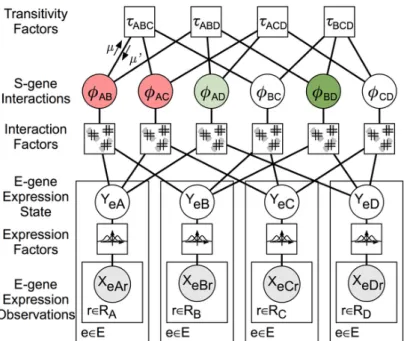
FG-NEM does model inference on a factor graph (Kschischang et al. (2001)). A factor graph is a bipartite graph with factors and variables as vertices. A factor and a variable are connected, if the factor includes the variable. A factor graph representing the example from figure 3.3 is shown in figure 3.4. The factor-graph encodes all possible networks at once. Variables (circles) are
• S-gene associations Φ = (ΦAB)
• hidden E-genes expression statesY = (YeA)withYeA as the hidden, discrete E-gene state of E-gene e during knock-downA and
• observed E-gene expressions X = (XeAr) with XeAr as the expression of E-gene e in replicate r of knock-down A.
Factors (boxes) are expression factors, interaction factors and transitivity factors. Ex- pression factors are Gaussian and connect the observed and the hidden E-gene state.
Interaction factors are the probabilities of the form
P (YeA, YeB|ΦAB,ΘeAB). (3.11) The maximum a posteriori is found using equations (3.9) and (3.10) and max-sum message passing (Kschischang et al. (2001)).
3.2.4 Dynamic Nested Effects Models
Original NEMs are designed for static experiments. After each experiment, the signalling pathway is assumed to be in a steady state. A steady state means every S-gene is in a final state of either 0 or 1 and there is no further change. As a result original NEMs cannot resolve feed forward loops. For example in case of the network A → B → C the original NEM cannot determine if the effect of A on C is direct or indirect via B.
Thus a feed forward loop from A→C is not resolvable under steady state assumptions.
Dynamic Nested Effects Models (D-NEM, Anchanget al. (2009)) extends NEM and uses timeseries data to infer time dependent signalling processes like feed forward loops.
Novel model parameters in D-NEM are the signalling rates K = (kij) of edges from S-genesitoj (figure 3.5). They are assumed to be exponentially distributed. K replaces
Figure 3.3: Predicting Pair-wise Interaction Using Quantitative Nested Effects.
(A) Hypothetical example with four S-genes, A, B, C, and D. The graph contains one inhibitory link, BxD (left). A heatmap of E-gene expression under knockdown of each S-gene shows both inhibitory and stimulatory effects (middle). Scatter plots of the C, A, B, and D knock-outs show that expression fits in the shaded preferred regions of each interaction (right). The inhibitory link explains some of the observed data: expression changes under DD (bright red or bright green entries in the heatmap) occur in a subset of the E-genes for which the opposite changes occur in DB. (B) Data from a known inhibitory interaction. Expression levels of effect genes under the DIG1/DIG2 knock-out (y-axis) plotted against their levels under the STE2 knock-out (x-axis) as detected in [17]. Expression changes significant at a = 0.05 indicated in gray lines. DIG1/DIG2 is known to inhibit STE12. (C) Interaction modes. Observed E-gene expression changes are compared to five possible types of interactions between two S-genes, A and B (iv). The top row illustrates the expected nested effects relationship for each type of interaction mode: circles represent sets of E-genes with expression changes consistent with either activation (blue circles) or inhibition (yellow circles). Scatter-plots for each interaction mode show the hypothetical expression changes under DA (x-axis) and DB (y-axis) for all E-genes (circles). E-gene levels are either consistent (filled) or inconsistent (open) with the mode. Shaded regions demark expression levels consistent with each interaction model. The example shows expression changes that most closely match the inhibition mode (indicated by the greatest number of closed circles). This figure was reproduced from Vaske et al. (2009).
Figure 3.4: Structure of the factor graph for network inference. The factor graph consists of three classes of variables (circles) and three classes of factors (squares). XeAr is a continuous observation of E-gene e’s expression under ∆A (knock-down of A) and replicate r. YeA is the hidden state of E-gene e under ∆A, and is a discrete variable with domain {up, , down}. ΦAB is the interaction between two S-genes A and B. Expression Factors model expression as a mixture of Gaussian distributions. Interaction Factors constrain E-gene states to the allowed regions shown in Figure 3.3. Transitivity Factors constrain pair-wise interactions to form consistent triangles. The arrows labeled µ and µ′ are messages encoding local belief potentials onΦAB and are propagated during factor graph inference. This figure was reproduced from Vaske et al. (2009).
Figure 3.5: Dynamic Nested effects ModelElementary example of a D-NEM. Shown is a network of three S-genes together with binary time series tables for typical E-genes connected to the S-genes. Each table holds three rows corresponding to the three possible perturbation experiments of S-genes. A one in column ti , rowSj of table Ek represents the observation of a downstream effect inEk ,ti time units after perturbation ofSj. This figure was reproduced from Anchang et al. (2009).
the model parameters Φ, which describe the S-gene topology. A large kij from S-gene i to j corresponds to a high signalling rate and an edge between the S-genes. A small kij objects any signalling from S-gene i toj. Therefore D-NEMs are parameterized by rate constants K and S-gene to E-gene connectivity Θas in 3.2.1.
The likelihood to score a candidate set K is defined as P(D|K,Θ) =∏
D=1
PSi→Ek(ts)(1−β) + (1−PSi→Ek(ts))α
×∏
D=0
PSi→Ek(ts)β+ (1−PSi→Ek(ts))(1−α).
α andβ are false positive and false negative rates. PSi→Ek(ts)is the probability, that the signal fromSi reaches Ekbefore timepointts. How this probability is calculated is shown in the following example.
Let’s assume we have the path g with a simplified index for the rate constants:
Si −→k1 Sj1· · ·−−→kq−1 Sjq−1 −→kq Ek.
Zg is the sum of of q independent, and exponentially distributed random variables with rate constants k1, . . . , kq. Zg’s targeted probability is P(Zg < ts). The density function of Zg is given by
Ψ(t)g =
∫∞ 0
· · ·
∫∞ 0
δ (
t−
∑q u=1
τu
) q
∏
u=1
Ψu(τu)dτ1. . . τq
with Ψu(τ) = kuexp(−kuτ) as the density of an exponential with rate ku. A Laplace transformation returns
Fg(t) =
∑q b=1
∏
a̸=b
{ ka ka−kb
}
[1−exp(−tkb)]
as a closed form for the cumulative distribution function ofZg. In the case of two or more ku with equal values the right side can be undefined. Anchang et al. (2009) avoid this by the use of small jitter values. Several paths can connect Si with Ek. For each path u Zu is constructed as before and the probability is given by
PSi→Ek(ts) = 1−∏
u
(1−Fu(ts)).
An optimal network model is inferred via a Gibbs sampling approach (George Casella (1992)).
3.2.5 Partial Nested Effects Models
Usually Nested Effect Models assume, that the pathway is isolated. That is only S- genes included in the model influence the signalling. This is not the case in general.
Literature is missing information on hidden players, which are not included in the model.
Additionally those players are not known to be missing. Sadeh et al. (2013) calls these players unknown unknowns and introduce Partial Nested Effects Models (P-NEM) as an extension to the original NEMs to account for them.
P-NEM looks for patterns in the data, which contradict certain hypotheses (edges) between two S-genes. For example let’s assume X is upstream of Y (M = X → Y).
E-genes reacting to Y but not X contradict that hypothesis, because if we knock-down X we indirectly knock-down Y given M. These contradicting effects are called a alien patterns. Every alien pattern in the data is tested for significance with a binomial test.
Alien patterns exists for four of five different edge relations between two S-gene (fig- ure 3.6, a). Each relation has its unique set of alien patterns except for the one in which X and Y have a common child (R5). This relation can explain all patterns.
For an example on how to detect significant alien patterns we look at relation R1.
Edge X → Y (R1) has three expected patterns and one alien pattern (X, Y) = (0,1).
The alien pattern can be the result of an expected pattern and noise (expected
noise
z}|{→ alien). If we consider a false positive rate α and false negative rate β, we can calculate the probability of each case:
• (1,0)
noise
z}|{→ (0,1)is the result of one false negative and one false positive and we have a probability of γ1 =β·α
• (1,1)
noise
z}|{→ (0,1)is the result of one false negative and one true positive and we have a probability of γ2 =β·(1−β)
• (0,0)
noise
z}|{→ (0,1)is the result of one true negative and one false positive and we have a probability of γ3 = (1−α)·α
We can now write an upper limit for the probability of more than k alien patterns in the data, given relation R1:
P (K ≥k|X →Y )≤
∑n i=k
(n i
)
γR1i (1−γR1)n−i (3.12) n is the total number of E-genes and γR1 an upper bound for the probability of observing an alien pattern. Such a bound for the probability is available for all relations except for R5, since it lacks an alien pattern. The other relations R1, R2, R3 and R4 are rejected if
P (K ≥k|Ri)< κ with κ as a cutoff for significance, e.g. κ= 0.05.
S1 S2
S1 S2
S1 S2
S1 NO RELATION S2
S1
H
S2
(a)possible relations R1 to R5
S2 S1
E1 E2 E3
S2 S1
E1 E2 E3
S2 S1
E2 E3
S2 S1
E1 E2 E3
S2 S1
E1 E2 E3 E4
(b)expected data patterns
S2 S1
E4
S2 S1
E4
S2 S1
E4 E5
S2 S1
E4
S2 S1
(c) unexpected alien patterns
S1
S2
H1 H2
H3 H4
H5 H6
H7
H8 H9
S1
S2
H1 H2
H3 H4
H5 H6
H7
H8 H9
(d) hidden nodes for re- lations R1 and R2
S2 S1
E1 E2 E3 E4 E5 E6 E7 E8 E9
S2 S1
E1 E2 E3 E4 E5 E6 E7 E8 E9
(e)data patterns for the hidden nodes
S1
S2
H1 H2
H3 H4
H5 H6
H7
H8 H9
S1
S2
H1 H2
H3 H4
H5 H6
H7
H8 H9
NO RELATION
(f) hidden nodes for re- lations R3 and R4
S2 S1
E1 E2 E3 E4 E5 E6 E7 E8 E9
S2 S1
E1 E2 E3 E4 E5 E6 E7 E8 E9
(g)data patterns for the hidden nodes
Figure 3.6: Partial Nested Effects Models Pairwise upstream/downstream relations and their alien patterns: (Top) Shown are the five possible possible relations (R1) . . . (R5) together with their expected silencing patterns and their alien patterns (grey are NA values). R4 are disconnected S-genes without indirect connections. (Bottom) Hidden vertices are introduced in all possible configurations, and the expected patterns of E-genes attached to the hidden vertices are shown. In (R4) the hidden vertex marked in red produces the alien pattern of (R4). Note that this constellation leads to the constellation in (R5). Based on figure 2 in Sadeh et al. (2013).