Oxygen in the Tropical Atlantic OSTRE Second Tracer Survey
Cruise No. M105
March 17 – April 16, 2014
Mindelo (Cape Verde) – Mindelo (Cape Verde)
M. Visbeck
Editorial Assistance:
DFG-Senatskommission für Ozeanographie
MARUM – Zentrum für Marine Umweltwissenschaften der Universität Bremen 2014
The METEOR expeditions are funded by the Deutsche Forschungsgemeinschaft (DFG) and the Bundesministerium für Bildung und Forschung (BMBF).
Editor:
DFG-Senatskommission für Ozeanographie
c/o MARUM – Zentrum für Marine Umweltwissenschaften Universität Bremen
Leobener Strasse 28359 Bremen
Author:
Prof. Dr. Martin Visbeck Telefon:+49-431-600-4100
GEOMAR Telefax:+49-431-600-4102
Helmholtz-Zentrum e-mail:mvisbeck@geomar.de
für Ozeanforschung Kiel
Standort Westufer Düsternbrooker Weg 20 24105 Kiel, Germany
Citation: M. Visbeck (2014) Oxygen in the Tropical Atlantic OSTRE Second Tracer Survey – Cruise No. M105 – March 17 – April 16, 2014 – Mindelo (Cape Verde) – Mindelo (Cape Verde). METEOR- Berichte, M105, 49 pp., DFG-Senatskommission für Ozeanographie, DOI:10.2312/cr_m105
_________________________________________________________________________________
ISSN 2195-8475
Table of Content
1 Summary ... 3
2 Participants ... 4
3 Research Program ... 5
4 Narrative of the Cruise ... 6
5 Preliminary Results ... 8
5.1 CTD system, salinity and calibration ... 8
5.1.1 CTD-system ... 8
5.1.2 CTD-conductivity calibration ... 9
5.1.3 Oxygen calibration ... 10
5.1.4 Salinometer measurements ... 10
5.1.5 Exemplary results ... 12
5.2 Vessel mounted ADCP ... 13
5.2.1 Exemplary Results ... 14
5.3 Underway Measurements (Thermosalinograph) ... 16
5.4 Underway pCO2, O2 and GTD Measurements ... 18
5.4.1 Preliminary results ... 19
5.5 Determination of dissolved Oxygen ... 20
5.5.1 Oxygen Winkler titration ... 20
5.5.2 Oxygen Optode Measurements on CTD –Casts ... 21
5.6 Measurements of CFC-12, SF6 and CF3SF5 ... 22
5.6.1. Methods ... 22
5.6.2 Preliminary Results ... 23
5.6.3 Tracer Loss Experiment (TLE) ... 28
5.7 Zooplankton Studies ... 29
5.8 Biological Incubation Experiments ... 31
5.8.1 N2 Fixation and primary productivity incubation experiments ... 31
5.8.2 Availability of excess P and DOP to primary producers in the Eastern Tropical North Atlantic (ETNA) ... 33
5.8.3 Dissolved organic matter supply to the Oxygen Minimum Zone ... 33
5.9 Particle Flux Measurements with drifting sediment traps ... 38
5.10 Determination of particulate organic matter and nutrients ... 40
5.11 Glider ... 40
6 Weather conditions during M105 ... 42
7 Station List M105 ... 44
8 Data and Sample Storage and Availability ... 48
9 Acknowledgements ... 48
10 References ... 48
11 Appendix – List of Abbreviations ... 50
1 Summary
Cruise M105 is a contribution to the German Research Foundation (DFG) Collaborative Research Project (SFB) 754: “Climate-Biogeochemistry Interactions in the Tropical Ocean” with the main goal to better understand the supply of oxygen to the oxygen minimum zone (OMZ) of the Tropical Atlantic with a particular focus on the role of regional advection, mesoscale and sub-mesoscale processes for lateral and vertical oxygen fluxes. A key method is the “Oxygen Supply Tracer Release Experiment” (OSTRE), where during M105 the second mapping of the tracer CF3SF5 using 160 CTD stations was done. Moreover mapping of the water mass properties, oxygen and transient tracer distribution were done. Several glider deployments and recoveries and the synoptic ocean circulation and mixing accomplished by S-ADCP observations, as well as glider based microstructure measurement were done. Finally a significant component of the cruise was dedicated to determine biogeochemical rates of oxygen consumption and nutrient cycling by zooplankton studies, nitrogen fixation experiments and two week long drifting sediment trap deployments. The cruise was very successful; all systems on METEOR worked well and all planned objectives were reached.
Zusammenfassung
Die Reise M105 wurde im Rahmen des DFG Sonderforschungsbereichs (SFB) 754: „Klima- Biogeochemische Wechselwirkungen im Tropischen Ozean“ durchgeführt, um die Belüftung der Sauerstoffminimumzone (OMZ) des Tropischen Atlantiks besser zu verstehen. Insbesondere der Einfluss der regionalen Zirkulation sowie mesoskalige und submesoskalige Prozesse auf den, horizontalen und vertikalen Sauerstofftransport wurden bestimmt. Eines der Schlüsselexperimente dazu liefert das “Oxygen Supply Tracer Release Experiment” (OSTRE), dessen zweite Vermessung auf dieser Reise durch 160 CTD Stationen erfolgte. Zudem wurden mehrere Gleiter ausgesetzt und aufgenommen. Die synoptische Zirkulation konnte mit dem S- ADCP und Gleiter-basierten Mikrostrukturmessungen erfasst werden. Weiterhin wurden diverse Messungen und Experimente durchgeführt, um biogeochemischen Sauerstoffzehrraten zu bestimmen. Nährstoffumsatzbestimmung konnten durch Zooplankton Experimente und Nährstofffixierungsraten durch Inkubationsexperimente und zwei Auslegungen driftender Sinkstofffallen ermittelt werden. Die Reise wahr sehr erfolgreich, alle Systeme der METEOR liefen gut und alle geplanten Ziele konnten erreicht werden.
2 Participants
Name Position/Discipline Institute
1. Prof. Dr. Visbeck, Martin Chief scientist GEOMAR
2. Dr. Tanhua, Toste Tracer GEOMAR
3. Dr. Schmidtko, Sunke CTD GEOMAR
4. M. Sc. Schütte, Florian CTD, SADCP, Glider GEOMAR
5. Link, Rudolf CTD GEOMAR
6. B. Sc. Maas, Josefine CTD GEOMAR
7. Barth, Juliane CTD GEOMAR
8. B. Sc. Vieira, Nuno CTD, O2 INDP – Instituto Nacional de Desenvolvimento das Pescas
9. Bogner, Boie Tracer GEOMAR
10. M. Sc. Köllner, Manuela Tracer GEOMAR
11. B. Sc. Vollmer, Thorsten Tracer GEOMAR 12. B. Sc. Waltemathe, Henning Tracer GEOMAR
13. B. Sc. Wiser, Lea Tracer GEOMAR
14. B. Sc. Rudminat, Francie Tracer GEOMAR
15. B. Sc. Hahn, Tobias pCO2, O2 GEOMAR
16. B.Sc. Christiansen, Svenja Zooplankton GEOMAR 17. B. Sc. Danelli, Maria Zooplankton GEOMAR 18. Dr. Wagner, Hannes Sedimenttrap GEOMAR
19. Roa, Jon Sedimenttrap GEOMAR
20. Dipl.-Biol. Meyer, Judith Biochemistry GEOMAR 21. M. Sc. Loginova, Alexandra Biochemistry GEOMAR
22. Dr. Singh, Arvind Biochemistry GEOMAR
23. B. Sc. Esser, Elisabeth Biochemistry GEOMAR
24. Heitmann-Bacza, Carola Meteorology DWD (Deutscher Wetterdienst) Hamburg
35. Stelzner, Martin Meteorology DWD Hamburg
GEOMAR GEOMAR Helmholtz Centre for Ocean Research Kiel, Düsternbrooker Weg 20, 24105 Kiel – Germany.
INDP Instituto Nacional do Desenvolvimento das Pescas , Rua: Cova de Inglesa, Mindelo, São Vicente, C.P: 132, Cabo Verde.
Scientific party of M105
3 Research Program
Cruise M105 is a contribution to the DFG Collaborative Research Project (SFB) 754: “Climate- Biogeochemistry Interactions in the Tropical Ocean”. The main goal of the study is to quantify and better understand the supply of oxygen to the oxygen minimum zone (OMZ) of the Tropical Atlantic with a particular focus on the role of regional advection, mesoscale and sub-mesoscale processes for lateral and vertical oxygen fluxes and thus a critical aspect of the ventilation of this region. One of the methods to derive oxygen transports is the “Oxygen Supply Tracer Release Experiment” (OSTRE), which allows the quantification of the time averaged diapycnal and lateral mixing rates in the region.
The main objective of the cruise was to:
a) perform the second mapping of the tracer CF3SF5 that was injected in late 2012 (MSM23) near the OMZ at around 10°N 21°W and about 500 meters depth;
b) map the water mass, oxygen and transient tracer distribution by the CTDs and glider;
c) determine the synoptic ocean circulation and mixing by S-ADCP observations, as well as glider based microstructure measurement;
d) determine biogeochemical rates of oxygen consumption and nutrient cycling by zooplankton studies, nitrogen fixation experiments and two drifting sediment trap experiments.
These objectives were addressed by a multi-disciplinary research program during M105 encompassing 160 CTD station, 23 zooplankton net hauls, underway ship-based measurements, glider deployments and recoveries and two short term deployments of drifting sediment traps.
Many biogeochemical analysis and experiments were carried out during the cruise.
In summary the cruise was very successful, all planned objectives were reached and the measurements were carried out as planned.
4 Narrative of the Cruise (Martin Visbeck)
R/V METEOR departed from Mindelo on March 17, 2014 at 9:00 and northward towards the Cape Verde Ocean Observatory (CVOO). On the way a gilder was released at 17°26’N and 24°30’W followed by a test CTD station.
The first CTD profile was malfunctioning. The failed CTD station was followed by a successful deployment of a multi-net cast. At CVOO the CTD station had to be aborted near the bottom because a deck unit computer failed and the connection could not be fully established.
Overheating of the sensors in the container was assumed to have caused the problems. New sensors were used from CTD profile 3 successfully.
METEOR ventured north to sample a low oxygen eddy that was discovered before by a glider and remote sensing. Two 40nm long transects centered at 19° 02’N and 24° 46’W with ten CTD stations will allow for a detailed description of this remarkable feature.
On March 19 a full ocean depth CTD cast was obtained at the CVOO. After a long transit towards southeast a glider was recovered at 16°N 33’ and 20°W 03’ on March 21 in the early morning. METEOR turned south and began early on March 22 a tracer sampling transect along 21°W with 30nm station spacing. Every 3 station a large number of biogeochemical parameter were sampled and a plankton net was taken. On March 23 we released two gliders at 11°N and 21°W one of which developed a leak and was recovered a few hours later. The reason might have been a leak in the science bay in the vicinity of the fluorometer. Unfortunately, one glider did not hold its vacuum, which suggests that there was a leak. All attempts to repair the gilder on board were not successful. Possibly overheating in the container during transport might have been a factor in the development of the leaks near the fluorometer at both gliders.
In the early afternoon we met with the German research icebreaker POLARSTERN and visits to the other ship were possible. On March 24 we released a drifting sediment-trap mooring at 10°N and 21°W. Midday on March 25 we reached the southernmost point a 7°N along the 21°W section and began steaming northward and completed the inner southeastern part of the survey grid.
On March 27 we reached 10°N and 21°W again and visually inspected the first drifting sediment-trap mooring. Shortly after that we deployed the second one at 10° 15’N and 21°W.
From there we began to complete the north-eastern part of the survey grid. On March 29 we reached the North East corner of the survey grid at 12°N and 19°W and in the evening the easternmost station at 11°N and 17° 30’W. On April 1 we recovered the first drifting sediment trap mooring in the afternoon and inspected the second on the way towards the southeastern part of the sampling grid. On April 3 we reached the south east corner at 8°N and 19°W of the survey grid and heading west. On April 4 midday we reached 7°N at 23°W and worked our way north in the western part of the sampling grid. In the morning of April 8 we deployed the last glider and recovered the sediment mooring #2 at 10° 38’N and 21° 30’W.
On April 10 we reached at 12°N and 23° the north-western corner of the survey box. From there we began a southward section along 24°W. On April 12 we reached 8°N once again and began our last section northward along 25°W. The last CTD station was taken at 8°N and 25°W in the evening of April 14.
METEOR arrived Mindelo in the morning of April 16.
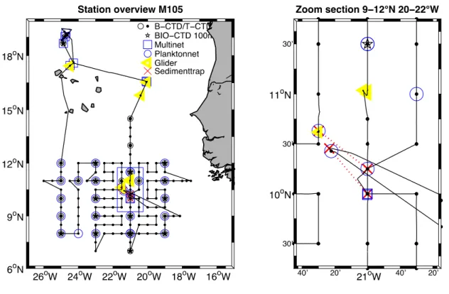
Fig. 4.1 Cruise track of METEOR cruise M105 with locations of CTD stations (small black dots), Bio-CTD (small black circle), WP2-Net (large blue circle), Multi-Net (blue square), drifting sediment trap (red crosses) and glider operations (yellow triangle).
5 Preliminary Results
In the following a detailed account of the types of observations, the methods and instrument used as well as some of the early results are given. Where appropriate the best practice suggestions for conduction high quality hydrographic observations as described in the GO-SHIP manual (Hood et al, 2010) were followed.
5.1 CTD system, salinity and calibration
(Sunke Schmidtko, Rudolf Link, Josefine Maas, Nuno Vieira) 5.1.1 CTD-system
During M105 a total of 160 CTD-profiles and 3384 water samples were collected. The rosette system was installed in a Seabird Rosette System frame for 24 bottles, but only 22 bottles 10 liters each were attached for the majority of profiles. The remaining two places were used for integrated water samplers from cast 12 till the end of the cruise. Integrated water samplers are syringes that do sample over 100 seconds and 200 seconds respectively and are solely analyzed for trace gases. See table below for sensor details. Depth profiles up to a maximum pressure of 5500 dbar were performed; for the majority of stations only the top 1200m of the water column was sampled. Data acquisition was done using Seabird Seasave software version 7.21k; pre processing was done with SBE Data Processing 7.21k.
The first CTD profile at instrument test station #178 was not recorded due to a deck unit malfunction. Nevertheless it was determined that both oxygen sensors attached to the CTD system SBE#7 at that time were malfunctioning.
The second CTD profile, during the first CVOO mooring site visit - station #179, used the alternative backup CTD system SBE#4. This system failed at depth of 3500m, 50m above the bottom. It was not possible to reestablish connection to the water sampler after restart of the system. No water samples were taken on the cast, thus this profile cannot be calibrated. Similar to profile 1 and CTD system SBE#7, malfunctions of both oxygen sensors (#145, #985) were determined.
All oxygen sensors (#145, #985, #2686, #2669) shipped in container PONU 068514-2 from Kiel to Mindelo had failed at first trial. Overheating in the container is assumed to have caused the problems.
From CTD profile 3, station #180, onwards CTD system SBE#7 was used again. For profile 3-5 the CTD system SBE#7 malfunctioning primary oxygen sensor (#2686) was replaced by an oxygen sensor from the R/V METEOR CTD system (#1812). The second malfunctioning oxygen sensor (#2669) was replaced following profile 5, station #182, by the second R/V METEOR CTD sensor (#1818). Both sensors stayed on the system until the end of the cruise and proved to be very reliable. The measurements from the primary sensor were chosen for the final data.
Due to erroneous configuration settings in the deck unit, profile 2-12 were recorded with 1sec bin averaging. Despite this sampling reduction of the vertical resolution, no significant reduction in data quality was observed. From profile 13 onwards all raw data were recorded at 24Hz.
At maximum depth of profile 19, station #194, there was a blackout of the acquisition computer of CTD deck unit 03. The cast was completed on CTD deck unit 06, which was solely
used there after. The up and down profile were successfully merged during past processing. The reason for the computer black out could not be determined, a possibility is that high laboratory air temperature (~40°C) might have caused a CPU cooling failure and lead to an automatic shut down.
The CTD system worked without problems for the final 141 profiles. The exact configuration of the CTD system can be found in table 5.1. Additionally a self-recording, self-powered Underwater Video Planktonrecorder, UVP, was attached to the water sampler. It is described separately in section 5.7.
Processed uncalibrated CTD data, 5-dbar binned, was sent in near real time to the Coriolis Data Centre in Brest, France, (via email: codata@ifremer.fr) for integration in the databases to be used for operational oceanography applications and the WMO supported GTS/TESAC system.
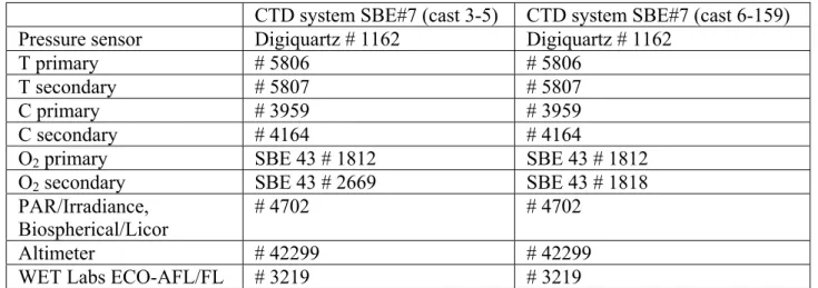
CTD system SBE#7 (cast 3-5) CTD system SBE#7 (cast 6-159) Pressure sensor Digiquartz # 1162 Digiquartz # 1162
T primary # 5806 # 5806
T secondary # 5807 # 5807
C primary # 3959 # 3959
C secondary # 4164 # 4164
O2 primary SBE 43 # 1812 SBE 43 # 1812
O2 secondary SBE 43 # 2669 SBE 43 # 1818
PAR/Irradiance,
Biospherical/Licor # 4702 # 4702
Altimeter # 42299 # 42299
WET Labs ECO-AFL/FL # 3219 # 3219
Tab. 5.1 Summary of CTD system SBE #7 configuration used during M105, PAR Sensor was removed for casts deeper 2000m (see station list section 7).
5.1.2 CTD-conductivity calibration
Overall 370 calibration points were obtained by sampling for salinity. Due to the large amount of samples a simple outlier removal method was applied that discharged the largest 40% deviations between CTD and bottle samples prior to calibration. The projection from the bottle stop of the up- to the downcast was done by searching for similar potential temperatures within 30dbar pressure internal around similar pressure horizons between up- and downcast. For the critical loop edit velocity 0.01m/s were used. The final CTD data set is composed from the secondary set of sensors for all profiles, though the differences between sensor pairs were marginal. The conductivity calibration of the downcast data was performed using a 1st order linear fit with respect to temperature, pressure and conductivity.
The calibration results in a salinity RMS-misfit for the downcast of order 0.00161 for the primary and 0.00154 for the secondary sensor. The upcast calibration succeeds these very good values with and RMS-misfit of 0.00158 for the primary and 0.00146 for the secondary sensor.
CTD system SBE#7
(profile 6 to 147) CTD system SBE#7 (profile 6 to 147)
Sensor pair primary secondary
RMS misfit after calibration - salinity 0.00161 0.00161 Polynomial coefficients - conductivity Offset: -0.001332
P1: -6.0356e-08 T1: -4.5593e-5 C1: 0.00068582
Offset: -0.0036883 P1: -6.9681-08 T1: -0.0001316 C1: 0.0014747 Pressure sensor correction (decks-offset) -0.46 -0.46
Tab. 5.2 End of cruise salinity and pressure summary of downcast calibration information for the two CTD systems used during M105.
5.1.3 Oxygen calibration
The CTD oxygen downcast for CTD systems is calibrated by using the best 60% of the joint data pairs between downcast CTD sensor value and titrated oxygen (Section 5.5). For the calibration a linear correction polynomial depending on pressure, temperature and the actual oxygen value was fitted. Due to the very accurate titration and stable oxygen data a marginal temporal drift was also detected. A total of 641 oxygen data points for CTD system SBE#7 were recorded, which results in an RMS-misfit for the downcast of the order of 0.57 µmol kg-1 for the primary SBE43 and 0.51 µmol kg-1 for the secondary SBE43. The upcast calibration even succeeded these very good values with and RMS-misfit of 0.49 µmol kg-1 for the primary SBE43 and 0.42 µmol kg-1 for the secondary SBE43.
Oxygen Sensor #1812 Oxygen Sensor #1818
8Sensor pair primary secondary
RMS misfit after calibration - oxygen 0.57 0.51
Polynomial coefficients - oxygen Offset: 1.8105 P1: 0.003819 T1: -0.09092 O1: 0.0069941 t1: 0.038742
Offset: 0.10512 P1: 0.0020414 T1: 0.022031 O1: 0.051911 t1: 0.065174
Tab. 5.3 End of cruise downcast oxygen summary of calibration information for the CTD system SBE#7 used during M105.
5.1.4 Salinometer measurements
(Josefine Maas, Nuno Vieira, PI: Martin Visbeck)
On board were two GEOMAR instruments Guildline Autosal salinometer #7 (Model 8400B, AS7) and #5 (Model 8400A, AS5). Both instruments were malfunctioning at first. It was
determined that during transport internal connections did come undone, thus the cell did not fill with sample water. After fixing the problem AS7 showed reasonable values but exhibited high drifts in salinity measurements and bath temperature over short measuring time periods so that the older instrument AS5 was used that had very stable values. AS7 had not been used afterwards.
The instrument has a manufacturer given accuracy in salinity of ±0.002. In total a number of 370 samples were measured from 141 CTD stations.
The bath temperature of AS5 was constant throughout the cruise with 24.519 °C and a standardisation of the instrument was performed at the beginning on 24th March using IAPSO standard sea water (batch: P155, K15: 0.99981) with a respective salinity of 34.9926. That value was set by adjusting a resistance to get the required conductivity measurement (potentiometer).
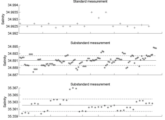
Furthermore a substandard, a large volume of water with constant salinity, was used to track the stability of the instrument. The substandard was obtained from CTD profile No. 30 from 1200 m depth.
The substandard showed no statistically significant trend in salinity during the measurements, comparison with standard with (batch: P155, K15: 0.99981) revealed that there is no instrument drift. Three standard measurements during the cruise showed slightly elevated values, though the final standard measurements showed similar values as for the start of the cruise. On 9th of April a new standardization was performed. The instrument showed an increase of about +0.0006 PSU.
During the whole cruise no drift of the device was detectable. Neither in the substandards (see Figure 5.1), which was in a nearly constant state, the standard (Figure 5.1) nor from the zero display which was ±0 throughout the measurements.
Fig. 5.1 Measurements of substandards and standard with AS5 during M105.
Salinity samples from the CTD and underway METOR TS recorder were analysed and the calibration procedures are described in section 5.1 and 5.3.
Additionally a Micro-salinometer from INDP Cape Verde was on board for comparison of instruments and determining its accuracy. The MS-310e Micro-salinometer (SN#015526) is based upon a concept in which conductivity of the sample seawater is simultaneously compared with the conductivity of standard seawater. The MS-310e uses two similar inductivity measuring channels to obtain a direct measure of the conductivity ratio Rtm. The two cells are maintained at the same temperature in a well-stirred oil bath.
The calibration of Micro-salinometer was done using IAPSO standard seawater (P153, K=0, 99979), and a routine standardization must be performed at least once in 24 hours, a second calibration used IAPSO standard seawater (P155, K=0, 99981). The offset from the MS3e- Micro-salinometer during the measurements was -0.004 with one standardization, and -0.0175 with another. It was demonstrated that good care needs to be taken to get high precision salinity values from this system.
5.1.5 Exemplary results
The sampling strategy of M105 data allowed the analysis of water mass distributions along two sections. The 11°N section (left panels, Figure 5.2) shows the west to east evolution across the Guinea Dome with the lowest dissolved oxygen concentration in the eastern part of the section.
The 21°W section (right panels, Figure 5.2) shows nicely the fading of the low salinity Antarctic Intermediate Water core towards the north. Several bands of high oxygen are visible above the OMZ with the highest oxygen values between 8° and 9° North.
Fig. 5.2 Top 1200dbar temperature, salinity and oxygen sections 11°N section, left panels, and 21°W section, right panels, through sample grid. The isopycnals of two tracer release experiments, OSTRE and GUTRE, are highlighted (white contours).
5.2 Vessel mounted ADCP
(Florian Schütte; PI: Martin Visbeck)
Underway-current measurements were performed continuously throughout the whole cruise using two vessel mounted Acoustic Doppler Current Profilers (VMADCP): a 75kHz RDI Ocean Surveyor (OS75) mounted in the ship’s hull, and a 38kHz RDI Ocean Surveyor (OS38) placed in
the moon pool. Both instruments worked well and produced good data for the duration of the cruise. The OS38 was aligned to zero degrees (relative to the ship's center line) in order to reduce interference with the OS75 that is aligned to 45 degrees.
Both instruments were run in the more precise but less robust broadband (BB) mode. The configurations of the two instruments are: OS38 using 80 bins of 16m, pinging at 25 per minute and OS75 using 100 bins of 8m, pinging at 35 per minute. Depending on the region and sea state, the ranges covered by the instruments are around 550m for the OS75 and around 1000m for the OS38. During the entire cruise the SEAPATH navigation data was of high quality. Most shipboard acoustic devises were switched of during the cruise to avoid acoustic interference.
Otherwise especially the Doppler Log and the multibeam echosounder would have produced significant interferences with the VMADCP’s. Only the 12kHz echosounder EM122 was in use during the whole cruise and delivered high quality bathymetry data without noticeable interference. One strong source of noise which affected or even destroyed especial the OS75 data, due to the position in the ship hull, was the bow thruster during stations. VMDAS software was used to configure the VMADCPs and to record the VMADCP data as well as the ships navigational data. The data were processed on board and a preliminary data set was used for a number of near real time velocity products.
5.2.1 Exemplary Results
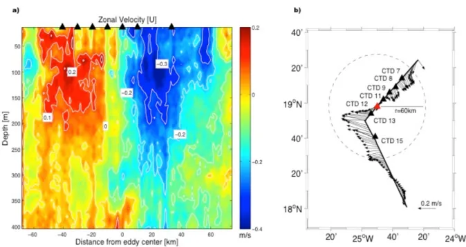
A VMADCP and CTD section was done to investigate an interesting mesoscale variability feature north of the Cap Verde Islands. The documented Anticyclonic-Mode-Water Eddy was observed since autumn 2013 with the help of satellite and glider data. It was generated near shelf break of the Mauritanian coast, most likely due to instabilities of the boundary current and traveled westwards along 18°N with a small deflection to the south. On average the eddy exhibited a westward propagation speed of 3km/day and needed around 8 months to travel to its recorded position. The anticyclonic rotation can be seen in a section crossing the eddy from northeast to southwest, showing the velocity structure in the upper 400 meters of the water column (Figure 5.3). In the CTD section the different water mass properties of the eddy are visible (Figure 5.4). Due to its rotation the original water mass (South Atlantic Central Water – SACW) is trapped in its core and transported into a region surrounded by a different water mass (North Atlantic Central Water – NACW). The oxygen concentrations inside of the isolated eddy core decreased with time due to biological consumption. After several weeks a thin layer of very low suboxic concentrations under 5µmol/kg developed centered at about 100m depths.
Fig 5.3 a) Zonal velocity from 0 to 400m depth during the eddy crossing, triangles indicated positions of CTD stations b) A map of the cruise track during the eddy crossing with the positions of the CTD stations (triangles) and the mean velocities vectors between 0 and 400m depth. The red triangle (CTD12) was near the core of the eddy and the circle indicates the possible shape oft he eddy with an estimated radius of 60km.
Fig 5.4 CTD section of a) temperature b) salinity and c) oxygen from 0 to 400m depth during the eddy crossing using CTD-Station 7, 8, 9, 11, 12, 13 and 15. The white contour lines represent the 26, 26.65 and 26.8 kg/m3 isopycnals.
5.3 Underway Measurements (Thermosalinograph) (Josefine Maas, PI: Martin Visbeck)
Underway temperature and salinity measurements were made with a SEABIRD Thermosalinograph SBE21 (Serial Number: 2149749-3313, see also METEOR Handbuch) installed in the ship’s port well about 5 m below sea surface. The instrument measures continuously sea water conductivity and temperature. From those the salinity is calculated. For calibration purposes of the conductivity sensor we took salinity samples every day during the entire duration of the cruise. Furthermore, the Thermosalinograph (TSG) data were compared to the results of the conductivity-temperature-depth (CTD) profiles.
During cruise M105 (March 17 to April 16), CTD measurements were performed in the tropical western Atlantic (17-25 °W) north of Cape Verde Islands and further south down to 7 °N. So we would expect elevated surface temperatures and salinity there what is confirmed by the TSG measurement. However in these months the coldest waters are encountered in these regions, ranging from sea surface temperatures (SST) 20.8 °C to 26.8 °C and typical sea surface salinity (SSS) characteristics ranging from 34.5 to 36.6 (Figure 5.5). Clearly visible is the typical higher practical salinity and lower temperatures on the first days near the Cape Verde Islands.
Fig. 5.5 Sea Surface Salinity (top) and Sea Surface Temperature (bottom). SSSs and SSTs from the ships Thermosalinograph (TSG) were compared to surface measurements of the CTD preliminary profiles (average of the upper 5 dbar) and also to salinometer measurements (green dots). TSG-measurements are denoted by solid lines, CTD-measurements by red crosses. Blue crosses denote stations that were excluded from calibration.
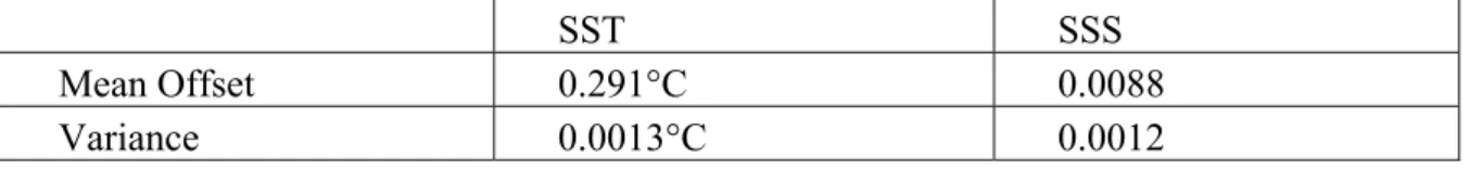
Good agreement was found between the reference measurements and the TSG data shown in Figure 5.5. Solid lines indicate measurements from the ship’s Themosalinograph, red crosses denote preliminary calibrated CTD-data that was averaged over the upper 5 db of the profiles. In SST measurements there is a constant offset visible of 0.291°C. Therefore the variance from the mean offset from TSG-data to CTD-data is very small, by only 0.0012 (Table 5.4).
SST SSS
Mean Offset 0.291°C 0.0088
Variance 0.0013°C 0.0012
Tab. 5.4 Surface temperature and salinity offsets and standard deviation calibrated against high accurate CTD data.
In the salinity time series from the TSG a linear decreasing trend of the values compared to CTD stations values is visible until the 31st of March (until CTD profile 74). At the beginning of the cruise SSS values were higher than CTD values, the week after the values were lower.
However, from the 31st March onwards there is very low variations between TSG and CTD salinity values visible (Figure 5.6). Therefore, it is reasonable to apply a linear fit to the first part of the time series while the second part can be adjusted with the mean deviation between CTD station data and the corresponding TSG value. There was no obvious explanation for this behavior of the sensor. Nothing was changed in the setup either on the CTD or TSG side. Note these are not The mean practical SSS offset is 0.0088 with a variance of 0.0012 (Table 5.4).
Comparison of these two quantities shows that practical TSG-salinity is on average a little higher relative to CTD-measurements by 0.008. TSG-temperature is on average higher than CTD-surface temperatures by 0.29°C (Figure 5.6).
Fig. 5.6 Difference between Thermosalinograph and CTD measurements for practical salinity and temperature [°C]. The solid line shows the average difference and the dashed line the standard deviation. Blue crosses are the deviations from the CTD stations, green dots are the deviations from the salinometer values. The vertical red line in the upper plot divides the time series into two sections. The first part can be adjusted 5by a linear time dependent fit, the second part was adjusted by the mean offset.
5.4 Underway pCO2, O2 and GTD Measurements (T. Hahn, T. Steinhoff, B. Fiedler, PI: A. Körtzinger)
Underway measurements of surface water pCO2 were performed using a commercially available GO-pCO2 measuring system (General Oceanics, Miami, FL). The instrument is described in detail in Pierrot et al. (2009).
A submersible pump and a temperature sensor (SBE38, SN# 3847374-0366, Sea-Bird Electronics Inc, Bellevue, USA) were installed in the ship’s moon pool at approximately 5 m depth. The pump supplied a continuous flow of surface water to the underway instruments (GO- System, through-flow box and bypass). A calibration of the Infrared (IR)-sensor was performed approximately every three hours by using three different standard gases containing ambient air with different partial pressures of CO2 (347.3, 450.2 and 670.8 ppm). The standard gases were calibrated against NOAA primary standards. After every control measurement, atmospheric pCO2 was measured for several minutes. Therefore air was pumped through a piping from the top of the ship. All temperature sensors were calibrated against international standards.
In addition 48 discrete samples for dissolved inorganic carbon (DIC) and total alkalinity (TA) were taken from the bypass and subsequently poisoned with HgCl2 following the recommendations of Dickson et al. (2007). The discrete samples will be analyzed in the laboratory at the GEOMAR in Kiel. The data from the autonomous measurements of the GO- system, which was recorded between Mar 17th 2014 at 11am (UTC) and Mar 18th 2014 at 8:25pm (UTC), need to be considered carefully due to a possible technical problem.
Underway measurements of surface water oxygen (O2), total gas pressure (GTD) and salinity were carried out in a flow-through box. The following sensors were implemented: Oxygen optodes (model 4330, SN# 1082, Aanderaa Data Instruments AS, Bergen, Norway; model Hydroflash O2, SN# DO-0314-001 and SN# DO-0314-003, CONTROS GmbH, Kiel, Germany), HGTD gas tension device (SN# 33-169-16, Pro Oceanus Inc., Bridgewater, Canada) and conductivity sensor (SN# 772, Aanderaa Data Instruments AS, Bergen, Norway).
84 discrete oxygen and 48 salinity samples were taken from the bypass to validate the underway measurements. Both types of samples were measured onboard using Winkler titration and the salinometer, respectively. The underway measurements in the flow-through box were stopped on Apr16th 2014 at 00:30 am (UTC). The data from the Aanderaa oxygen optode, which was recorded between Mar 17th 2014 at 11am (UTC) and Mar 19th 2014 at 1:12pm (UTC), must be considered as erroneous due to a technical problem.
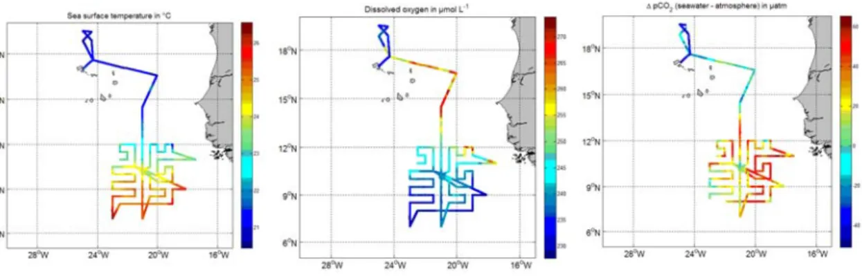
5.4.1 Preliminary results
Figure 5.7 shows preliminary and uncalibrated underway data of ∆pCO2, SST and O2. The SST shows the expected pattern with warmer water at the tracer grid between 24°C and 26°C and colder water in the northern part of the cruise track. The surface water O2 data are following the temperature pattern during most parts of the cruise track. pCO2 generally shows super-saturation due to the warm temperatures along the tracer grid, but between 18°N and 15°N, under- saturation (with respect to the atmosphere) was also observed.
Fig. 5.7 Preliminary underway data of SST, oxygen concentration and ∆pCO2 (seawater pCO2 – atmospheric pCO2). Note: the early gas data between Mindelo and the Eddy are erroneous.
5.5 Determination of dissolved Oxygen 5.5.1 Oxygen Winkler titration
(T. Hahn, T. Tanhua)
Observing and understanding the concentration of dissolved oxygen in the ocean is one of the key objectives of the SFB754. While the CTD system is capable to measure dissolved oxygen in the ocean at high vertical resolution, the sensors need to be carefully calibrated. Thus high quality reference observations are essential.
Oxygen measurements:
A total amount of 812 discrete water samples were taken from selected depths for oxygen measurements by Winkler titration. Samples were taken with 100 ml WOCE bottles with well- defined volumes (calibrated flasks) from the majority of the CTD rosette casts in order to calibrate the SBE43 oxygen sensors attached to the CTD. Oxygen samples were taken immediately after tracer sampling. It was ensured that the sample bottles were flushed with at least 3 times its volume and the samples were free of air-bubbles. At most CTD casts, a duplicate from one of the Niskin bottles was taken in order to quantify sampling and titration uncertainties.
Additional 84 water samples were analyzed from the underway system (see chapter 5.4 for further details) to calibrate and verify the underway oxygen sensors.
Oxygen was determined by Winkler titration within a maximum of 16 hours after sampling following standard protocols (Langdon, 2010). The concentration values were reported in µmol · kg-1. The precision of the Winkler-titrated oxygen measurements (1σ) was 0.34 µmol · kg-1 based on 140 duplicates and 1 triplicate. By comparing the standard solution with independent reference materials from WAKO inc. (Japan), the standard solution KH(IO3)2 was found to be accurate to better than 0.02 % (0.01 μmol · kg-1).
Measurement setup:
The following reagents were used during this cruise:
sulfuric acid (50%)
zinc iodide starch solution (500 mL, Merck KGaA)
stock solution: sodium thiosulfate pentahydrate (49,5 g ·L-1); stock solution was diluted by a factor of 10 to create the working solution (0.02 mol·L-1)
fixation solution: manganese(II)chloride (600 g ·L-1), sodium iodide (600 g ·L-1) and sodium hydroxide (320 g ·L-1)
standard solutions: potassium hydrogen diiodate (0,325 g·L-1, homemade) and potassium iodate (CSK Standard Solution, 0.01N, 300 mL, Wako Pure Chemical Industries, Ltd., Japan)
Titrations were performed within the WOCE bottles using a 20 mL Piston Burette (Nr. M 005684) TITRONIC universal from Schott Instruments. Dosing accuracy reported the company indicates 0.15%, referred to the nominal volume, as a measurement uncertainty with a confidence level of 95%. The iodate standard was added with a 50 mL Piston Burette (Nr. M 001545) TITRONIC universal from Schott Instruments. 1 mL of the fixation solutions
(NaI/NaOH and MnCl2) were dispensed with a high precision bottle-top dispenser (0.4-2.0 mL, Ceramus classic, Hirschmann).
Titration procedure:
The titration procedure for each measurement was the following:
1) Switch on Piston Burettes and clear the system (dosing tubes) from air bubbles
2) Determine factor of the thiosulfate working solution by titrating the homemade standard between 3 to 5 times on a daily basis
3) Measure the actual Winkler samples
4) Analyze the reagent blank at the beginning and the end of the research cruise; Compare homemade standard with the WAKO standard at least three times throughout the cruise Note: Possible sampling, storing (air bubbles) or measuring failures were recorded. Results derived from those measurements were not considered in the data evaluation.
5.5.2 Oxygen Optode Measurements on CTD –Casts (T. Hahn, C. Frank, H. Bittig, PI: A. Körtzinger)
Optical oxygen measurements with a new prototype oxygen optode (model: Hydroflash O2, SN#
DO-0314-002, CONTROS GmbH, Kiel, Germany) were carried out on 8 CTD – casts in order to characterize its performance. CTD – profiles 191-2, 192-2, 198 and 201-3 were used to determine the response signal during the up- and downcast of the CTD. Therefore, the optode was attached close to the inlet of the SBE43 for comparison.
To determine the optode behavior under changing pressure but constant oxygen, temperature and salinity conditions, the optode was attached inside a Niskin bottle to the upper spring. Niskin bottle 1 was used during CTD – profile 281-3, and Niskin bottle 4 during CTD – profiles 285 and 295. As a first order assumption, salinity and oxygen are constant after closure of the Niskin bottle and changes of temperature are assumed to be small and slow. Thus, deep ocean conditions >3000dbar serve as a first order pressure calibration with no concurrent changes in other parameters.
Furthermore, CTD – profile 320-2 was used to observe the signal of the optode in a low oxygen environment. Therefore, the optode was attached inside Niskin bottle 11, which was closed in the depth of the Oxygen Minimum Zone.
All data during each CTD – cast were logged internally with the optode using the power supply of a manufacturer customized battery module. Furthermore, the oxygen optode was calibrated onboard at three different temperatures each at two saturation levels (0% (Na2SO3) and 100%).
5.6 Measurements of CFC-12, SF6 and CF3SF5
(B. Bogner, M. Köllner, T. Tanhua)
Measurements of the deliberately released tracer CF3SF5 in an area around the position where the tracer was released during the MSM23 cruise in December 2012 was one of the primary goals of the M105 cruise. In this area a grid of CTD stations within a 4x4° box, between 19-23°W and 8- 12°N, was measured with emphasis of the depth layers around the potential density anomaly (σθ) where the tracer was released, 27.03 kg m-3.
5.6.1. Methods
During the cruise, two GAS CHROMATOGRAPH / PURGE-AND-TRAP (GC/PT) systems were used for the measurements of the transient tracers SF6, CFC-12 and the deliberately released tracer CF3SF5. The systems are modified versions of the set-up normally used for the analysis of CFCs (Bullister and Weiss, 1988). Two almost identical instruments, PT3 and PT4, were used during the cruise. Unfortunately the chromatography on PT4 did not allow for evaluation of the SF6 peak, probably due to slightly differently packed GC columns. Therefore most shallow (generally from 150 meter and upwards) samples were measured on PT3; above this depth the use of CFC-12 as a transient tracer is limited, below this depth the uncertainty of SF6 is larger due to the low concentration. At the “CVOO” station one profile was flame-sealed in ~350ml ampoules, in addition to measurements on-board, for measurement onshore at GEOMAR for the measurement of novel transient tracers.
The traps for both systems consisted of 100cm 1/16” stainless steel (SS) tubing packed with 70cm Heysep D kept at about -70°C during trapping in the fumes over liquid nitrogen (LN2), and desorbed at 130°C. The gas chromatographic pre-columns consisted of a porasil C front-end with a molecular sieve 5A tail-end, for PT3 45+45 cm and for PT4 20+20 cm in 1/8” SS tubing.
The main column for both systems was 200 cm carbograph 1AC front-end and a 20 cm molecular sieve tail-end, in 1/8” SS tubing. With this set-up PT 3 was operated isothermal at 60°C and PT4 isothermal at 50°C. The differences between the two systems were due to slightly differently packed columns. Detection was performed on an Electron Capture Detector (ECD) kept at 300°C.
Samples were collected in 250 ml ground glass syringes either from the Niskin bottles or the sample was drawn directly into the syringe on the Rosetta under water with the “integrated sampler”. This was a device mounted on the Rosetta instead of the Niskin bottles 22 and 24. On the trigger command from the CTD deck unit a motor started slowly, but controlled, to fill the syringe. The speed of the motor could be controlled, and was set such that one of the samples was collected in a 200-meter depth interval (±100 meter) around the target density, whereas the other sample was taken in a narrower (100 meter) depth interval. Rather, since only the speed and the duration of the motor was controlled, the exact depth range sampled depended on the speed of the CTD on the up-cast. The purpose of these samplers was to measure the average CF3SF5 concentration in the tracer depth range with the aim to calculate the column integral of the tracer. An aliquot of about 200 ml of the samples (both discrete and integrating) was injected into the analytical systems. The purge towers of the two systems were 200 and 250 ml for PT3 and PT4, respectively.
Standardization was performed by injecting small, but accurately known, volumes of gaseous standard containing SF6, SF5 and CFC-12, a working standard prepared by the company Dueste- Steiniger (Germany). The CFC-12 and SF6 concentration in the standard will be calibrated vs. a reference standard obtained from R.F Weiss group at Scripps Institution of Oceanography (SIO) post-cruise. The CF3SF5 concentration was calibrated vs. another standard from Dueste-Steiniger that has been used on previous cruises during Guinea Upwelling Tracer Release Experiment (GUTRE) and OSTRE. Calibration curves were measured about once weekly to characterize the non-linearity of the system, depending on workload and system performance. Point calibrations were always performed between stations to determine the short-term drift in the detector.
Replicate measurements were only taken on a several stations and the so determined values for precision are listed in Table 5.5.
Compound PT3
precisions PT4
precisions Detection limits
SF6 0.03 fM
2.8 % NA 0.05 fM
SF5 0.05 fM
2.2 % 0.09 fM
2.1 % 0.07 fM
CFC-12 9 fM
1.3 % 4 fM
0.9 % 0.1 fM
Tab 5.5 Precision of tracer measurements determined from replicate measurements. The relative precisions are representative for samples with higher concentrations, the absolute values for low concentration samples (all concentrations in fmol kg-1). The inter-system precision is based on double samples analyzed on both instruments. The detection limit is the lowest concentration detectable; the limit of quantification is roughly 5 times that. No CFC-12 samples below 5 fmol kg-1 were measured, i.e. well above the quantification limit.
5.6.2 Preliminary Results
On a total of 160 stations discrete samples were taken and on 103 stations integrated samples were taken in addition. More details about the number of measurements are listed in Table 5.6.
PT3 PT4
# of measured samples 1474 1073
# of standard curves 5 5
# of duplicate measurements 55 32
Tab 5.6 Number of measured water samples, including number of duplicate samples; duplicate measurements include measurements from the surface or deep layers containing no CF3SF5.
All CFC-12, SF6 and CF3SF5 measurements plotted vs. density are shown in Figure 5.8 Concentrations up to about 30 fmol kg-1 for CF3SF5 were found during the cruise. For each station, the maximum CF3SF5 concentration was mostly found in a tight range around the target density anomaly of 27.03 kg m-³, on which the tracer was released in December of 2012. The long “tail” of the CF3SF5 distribution on lower densities is a tell-tale of the CF3SF5 tracer that was released in April 2008 for the GUTRE experiment. The tracer for GUTRE was released at 8°N, 23°W at the potential density anomaly 26.86 kg m-³. The remains of that experiment shows up on all profiles within the area as an almost constant background with peak concentrations of about 1 fmol kg-1. The distribution of the GUTRE tracer in the upper bounds of the density interval allow us to calculate the vertical dispersion of the tracer 6 years after injection, complementing previous studies (e.g. Banyte et al., 2012). Since the concentration of the
“GUTRE tracer” is similar on all stations, a background concentration can be removed from all profiles in order to make a distinction to the “OSTRE tracer”.
Fig. 5.8 Plots of the preliminary data of transient tracers (CFC-12 and SF6, left panels) and the deliberately released tracer CF3SF5 (top right panel) vs. potential density (σθ). All measured values of the cruise are plotted in gray in the background. The black dots indicate the measurements at an exemplary station (CTD profile 111). The black dots in the map (lower right panel) indicate the location of the stations where tracers were measured.
The vertical distribution of the CF3SF5 is at this time, 15-16 months after injection, was close to Gaussian (plotted vs. density) at almost all stations, even though the magnitude of the peak varies significantly. We encountered non-Gaussian distributions only at a few stations. We
calculated the column integral of the tracer, i.e. amount of tracer per unit area (nmol m ) by interpolating the discrete measurements. The column integral can also be calculated with help of the data from the integrated samples, and preliminary result suggests a good match between the two approaches to calculate the column integral (not shown). This is the primary quantity that will be used for calculation of the horizontal dispersion of the tracer. The lateral distribution is visualized in Figure 5.9.
In this respect it is interesting to note that the peak concentrations found during this cruise (~30 fmol kg-1) are 4-5 times higher than those found 18 months after the release of a similar amount of tracer during the GUTRE experiment (~6-7 fmol kg-1). The initial results suggest that the OSTRE tracer could be found at almost all stations within the 4°x4° “box” that we sampled extensively, but that the column integral of the tracer is still highly variable. During the cruise we could detect CF3SF5 at all stations south of the CVOO station, although for several stations we were only able to detect tracer from the GUTRE experiment, see Figure 5.9.
Fig. 5.9 Tracer column integral of CF3SF5 in nmol m-²: A “background” value of 0.17 nmol m-2 has been subtracted from each station as the remains of tracer from the GUTRE experiment. White dots are stations where no tracer was found.
Figures 5.9 and 5.10 shows the vertical distribution of CF3SF5 in fmol kg-1 along two sections; along 11°N and along 21°W. These two sections were both sampled outside of the main survey area bounded by 8-12°N and 19-23°W. Both sections show that the tracer has spread in separated small patches with local maxima of more than 20 fmol kg-1. The tracer concentration reduces to below the detection limit roughly 100 m below the target density, but is detectable roughly 200m above the target density, due to the presence of the tracer from the GUTRE experiment that was injected at a lower density (depth). A number of sections can be drawn from these data along various longitudes and latitudes.
Fig. 5.10 Depth section of CF3SF5 concentrations along 21° 00’ W. Dots indicate positions of measurements.
The tracer is confined in a depth layer around the target density of 27.03 σθ.
Fig. 5.11 Depth section of CF3SF5 concentrations along 11° 00’ N. Dots indicate positions of measurements.
The tracer is confined in a depth layer around the target density of 27.03 σθ.
During the M105 and M97 cruises a total of five full depth stations were sampled for measurement of CF3SF5 close to the tracer injection site. On the three stations closest to the injection site we did find tracer concentrations in the sub-femtomolar range, Figure 5.12. It appears that a small amount of tracer fell through the water column and dissolved close to the bottom. These data will serve as a base for calculating the amount of tracer lost during injection in order to better constrain the amount of tracer injected on the target density. No tracer was found in the water column between the bottom and the OMZ.
Fig. 5.12 Concentration of CF3SF5 at five deep stations sampled during M105 and M97 close to the tracer injection site from 2012. Left panel, CF3SF5 concentrations in the deep water column; Right panel, positions of the deep stations, the tracer injection is marked with gray lines. Profiles where we found deep tracer are marked with black dots.
5.6.3 Tracer Loss Experiment (TLE) (M. Köllner)
During tracer release experiments it is commonly observed that the peak of the tracer concentration is found at slightly higher density than at which it was injected. The cause of this has never been fully explained, but various explanations ranging from 1) gravitational sinking of droplets of tracer shortly after injection before fully dissolved (the tracer has a high density in its liquid form), 2) absorption onto sinking organic particles, and 3) an effect of turbulence induced by the injection sled. Experiments were undertaken during the cruise in order to quantify the effects of absorption onto biological particles. It has been shown that loss of CFC tracers from the photic zone, and subsequent desorption in the deeper part of the water column, can be a significant process in coastal, particle rich, environments (Tanhua and Olsson, 2005). The question is if this process can be of significance in particle poor environments with very high tracer concentrations shortly after the injection. Quantification of tracer transport through sinking particles will reduce the uncertainties of Tracer Release Experiments, particularly for the vertical advection term but also for calculations of vertical diffusivity. This experiment was funded as a PhD project by SFB754 and carried out by Manuela Köllner.
Four experiments were conducted during the cruise. For every experiment three 250 ml ground glass syringes were filled with 50 ml CF₃SF₅ - free water enriched with phytoplankton.
Three syringes were prepared with 50 ml filtered (0.2µm filter) CF₃SF₅ - free water as control samples. Additionally three 500 ml glass bottles with ground glass stoppers were filled with 50 ml phytoplankton-enriched water and 200 ml of filtered CF₃SF₅ - free water. At four stations the syringes were filled with additionally 200 ml of water from a Niskin bottle closed at or around the OSTRE target depth were the highest CF₃SF₅ concentration were expected. The syringes and bottles were stored in a 10°C temperature-controlled room attached to a plankton-wheel to keep the samples well mixed. The samples were measured in the lab after 16-24 hours of incubation in
the cool-room. The water from the syringes was measured with the GAS CHROMATOGRAPH / PURGE-AND-TRAP (GC/PT) system, see section 5.6.1. In order to protect the analytical system from a high particle load, all TLE-samples were pressed through a 0.45µm gas tight filter unit.
The samples in the bottles were filtered through 0.2 µm filter and the filter were subsequently frozen and stored for post-cruise mass determination in Kiel. Preliminary results indicate that the samples incubated with phytoplankton have approximately 8% lower concentration compared to the control, Figure 5.13. With knowledge of the mass of phytoplankton in the samples, the bioaccumulation factor for CF3SF5 can be calculated.
Fig. 5.13 Normalized concentration of CF3SF5 in the four experiments. The concentration of the control run is normalized, the error-bar indicate the spread of the triplicate samples.
5.7 Zooplankton Studies
(Svenja Christiansen, Maria Danelli, PI: Helena Hauss)
The zooplankton investigations focused on three aspects. With an Underwater Vision profiler (UVP) fine-scale vertical profiles of particle and zooplankton distribution were obtained at first.
Second, stratified sampling with a Hydrobios Multinet was carried out to address taxonomy and vertical distribution of zooplankton in larger depth intervals, specifically focusing on day/night differences at the same site. The third topic concentrated on spatial variability of excretion rates of the epipelagic copepod species Undinula vulgaris that was caught with a WP2 plankton net.
In total 145 UVP profiles, 10 Multinet hauls and 24 WP2 net hauls were completed.
Particle and Zooplankton observations with the Underwater Vision Profiler:
An Underwater Vision Profiler 5 (UVP), serial number 10, was mounted on the CTD-rosette.
The UVP consists of one down facing HD camera in a pressure-proof case and two red LED light arrays, which illuminate a defined water volume. During the downcast of a CTD- deployment, the UVP takes 3 to 11 pictures of the illuminated field per second. For each picture, particles larger than 60µm are sized and counted. Furthermore, images of particles with a size >
500 µm are saved as separate “vignettes” - small cut-outs of the original picture – which allow
for later, computer assisted identification of these particles and e.g. their grouping into different particle, phyto- and zooplankton classes.
In total 145 UVP profiles were taken on 161 CTD-stations during M105; 10 of them to the bottom depth (between 1400 m and 5200 m) and 101 to a depth of 1200 m. 15 casts went to 100 to 130 m depth. At four stations, the UVP recorded no data due to technical problems with the power cable shunt and at 11 stations due to other technical problems. The UVP was run autonomously and a specific depth routine was carried out to start it: The CTD was lowered to 10 m, stayed there for about one minute to enable the power up of the UVP, was sent to 20 m depth to start image acquisition and after that was heaved to the surface and then began the actual downcast.
All measurements were taken with the same configuration settings of the UVP, the most important ones are shown in table 5.7, and a well-defined distance between the camera and the lights of 36 cm.
Lens_model Tamron Lens_focal 8
Fovx 188
Fovy 141
Pixel 151
Focal_distance 375
Aa_calib 32
Exp_calib 13.603
Img_Vol 93
Tab. 5.7 Main parameter setting for the UVP 5 system.
MultiNet deployment:
MultiNet hauls were carried out at three stations in the investigated oxygen depleted anticyclonic modewater eddy, at the Cape Verde Ocean Observatory site (CVOO, 17°35‘N 24°17‘W) and at one station near the African shelf (16°33‘N 20°2.7‘W) and at the first sediment trap deployment site (10°N 21°W). At the first CVOO station only a day haul was carried out, the eddy was sampled near the core during the day, in the core at night and at the margin during the day. The other stations were sampled with one day and one night haul. A HydroBios MultiNet Midi with 0.25 m2 mouth opening, five separate nets, and 200 µm mesh size was deployed vertically down to a maximum sampling depth of 600 m in the eddy, 800 m at CVOO and 1000 m at the other stations. In the eddy, sampling intervals were chosen according to hydrographic conditions obtained from a CTD cast shortly before the first MultiNet deployment. The chosen depths were 600-300-200-120-85-0 m in order to discern the layer of lowest oxygen values in the shallow OMZ (120-85 m). At CVOO, defined standard depths were used (800-600-300-200-100-0 m) that are consistent for the time series carried out at this station. At the other stations, the defined standard depths were 1000-600-300-200-100-0 m, which have already been used during cruises MSM22 (Nov 2012) and M97 (June 2013) in the area. With these depths, one net contained a part of the zone below the oxygen minimum zone, one covered the deep OMZ, one the oxycline, one the layer below the mixed layer and one the well ventilated, highly productive surface layer.
The net was lowered to 100 m with a speed of 0.5 m s-1 and then with 1 m s-1. It was heaved with 1 m s-1. Before heaving to deck it was thoroughly rinsed with seawater to collect all zooplankton
in the cod end. Samples were stored in 100 ml Kautex bottles in a 4% Formaldehyde in seawater solution. Samples will be transported to the laboratory at INDP, Mindelo, and analysed there using the Zooscan method.
When visually inspected, zooplankton abundance in the day and night samples showed clear signs of diel vertical migration with higher abundance in the surface layer during the night. In the core of the Eddy, where oxygen values below 5 µmol kg-1 were registered, the surface net caught large numbers of zooplankton. Gelatinuos zooplankton (Siphonophora and medusa) was especially abundant. All other nets contained lower biomass than that outside the eddy, and even in the absolute oxygen minimum zone (between 120 and 85 m depth) living zooplankton was found.
Zooplankton excretion experiments:
At a total of 24 stations, distributed over the whole station grid, samples with a WP2-plankton net were taken from the upper 100 m. The vertical hauls were done at a lowering and heaving speed of 0.2 m s-1 to keep the stress level for the animals low. Once on deck, the cod end was removed and immediately transferred into a bucket of seawater. From these samples, 25 copepods of the species Undinula vulgaris were sorted out and groups of five incubated in filtered seawater at 23°C. From the incubation bottles water samples were taken right before the insertion of the copepods and then every 2.5 hours (in total 4 times) and ammonium and phosphate concentration were measured.
Ammonium was measured immediately after a method by Holmes et al. (1999) and phosphate following Grasshoff et al 2007 (Hansen and Koroleff, 2007). 22 Experiments were completed, at one station (12°N 19°W) no specimens of Undinula vulgaris were found and at one station (12°N 25°W) almost every copepod in the sample was dead maybe due to contacts with gelatinous organisms that were also caught with the net.
After the incubation, the copepods were dried at 50°C to enable dry weight determination ashore. The weight corrected ammonium and phosphate concentrations will be used to calculate the excretion rate of U. vulgaris in different areas of the working grid and will be compared to the POM concentrations that were found in the water samples from the CTD. Zooplankton was not caught quantitatively with the WP2, but observations showed a gradient in total biomass across the grid with highest biomass in the northeastern part and lowest in the south and west.
Also the diversity seemed to be higher in those regions.
5.8 Biological Incubation Experiments
5.8.1 N2 Fixation and primary productivity incubation experiments (Arvind Singh, PI: Ulf Riebesell)
Recent studies (e.g., Großkopf et al., 2012) have highlighted the problems associated with the earlier method of estimating N2 fixation (e.g. equilibration of 15N2 gas tracer). A new methodology, which was recommended by Mohr et al. (2010), was adopted in the present expedition. The sampled area during this cruise has been surveyed by biogeochemists because it receives ample amount of nutrients through upwelling, which leads to less chances of N2


![Fig. 5.6 Difference between Thermosalinograph and CTD measurements for practical salinity and temperature [°C]](https://thumb-eu.123doks.com/thumbv2/1library_info/5488398.1685068/19.892.107.734.123.600/fig-difference-thermosalinograph-ctd-measurements-practical-salinity-temperature.webp)