The measurement of pH in saline and hypersaline media at sub-zero temperatures:
Characterization of Tris buffers by Stathys Papadimitriou, Socratis Loucaides, Victoire Rérolle, Eric P. Achterberg, Andrew G. Dickson, Matthew Mowlem, Hilary Kennedy
Supplementary Information
This section includes the e.m.f. measurements in solutions of HCl in synthetic seawater (S = 35) and in synthetic seawater-derived brines (S = 45 – 100) in cells (B) and (C), respectively. These measurements, along with salinity, temperature, and pertinent solution composition information, are given in Table S1 below; they were used to determine the apparent standard potential (
E
o¿ ) ofcells (B) and (C) in the presence of sulphate in the synthetic solutions of this study as described in the section The apparent standard potential of the Harned cell with synthetic seawater (S = 35) and synthetic brine (S > 35) of the main article. This is followed by information about the standard error from the Regression output of individual fitted coefficients of equations (1) to (3) (Table S2), described in the section The standard potential of the Harned cell to the freezing point of synthetic seawater and brines, and equations (4) to (8) (Table S3), described in the section The pH of Tris buffers to the freezing point of synthetic seawater and brines.
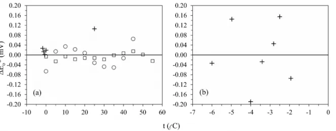
This section also includes plots of the residuals in Eo¿ as a function of temperature between the experimental values and fitted values (a) from equation (1) for seawater (S = 35) and temperatures from 55 to –1.7 °C, and (b) from equation (2) for seawater and brines at their freezing point (Fig. S1). Finally, the residuals in pHTris as a function of temperature are shown in Figure S2 between the experimental values and fitted values (a) from equation (4) for the equimolal Tris buffer (molality ratio, RTris = mTris/ mTris−H+ = 1) in seawater (S = 35) at temperatures from 45 to – 1.7 °C, (b) from equation (5) for the equimolal Tris buffer in seawater and brines at their freezing point, and (c) from equation (6) for the non-equimolal Tris buffer (RTris = 0.5) for seawater and brines at their freezing point.
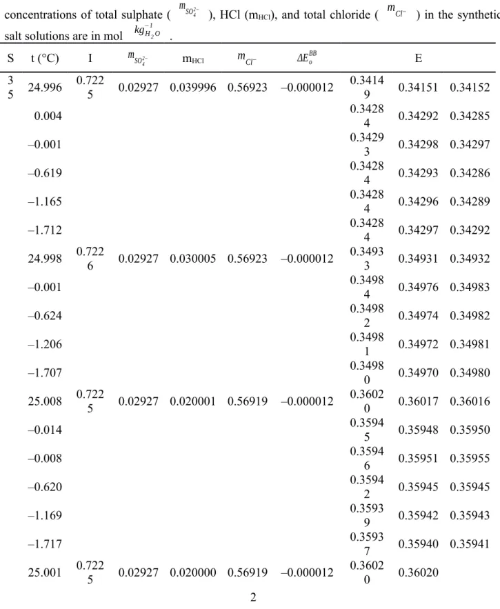
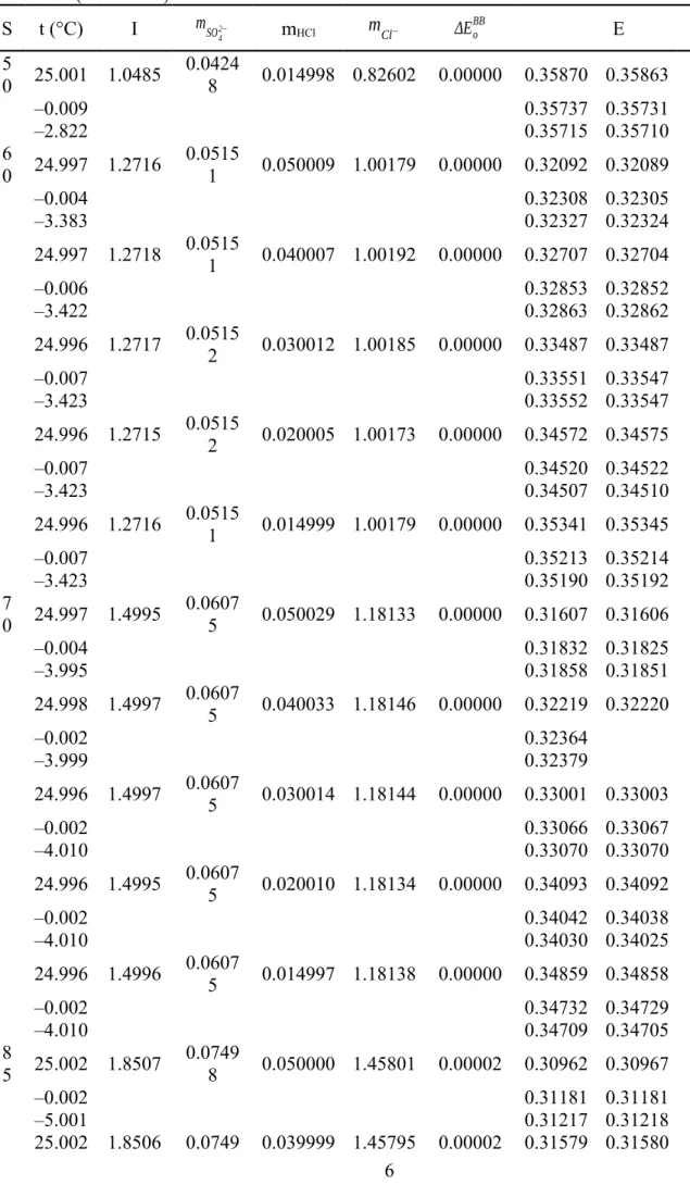
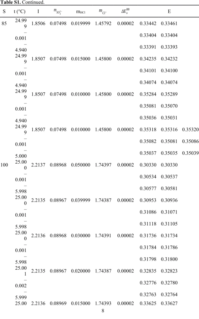
Table S1. The e.m.f. (E, in V) of the Harned cell with HCl solutions in synthetic seawater (S = 35) and synthetic seawater-derived brines (S > 35). The reported E values were corrected to a hydrogen fugacity of 101.325 kPa and were adjusted to the Eo of Bates and Bower (1954) ( EoBB ), with EoBB computed from the relevant temperature function in Dickson (1990b) (e.g., EoBB = 0.22240 V at 25
°C and 0.23659 V at 0 °C). The adjustment to EoBB was done using the average difference ( ΔEoBB , in V) of EoBB from the Eo values ( Eomeasured ) derived from e.m.f. measurements of dilute HCl solutions in de-ionized water at 0, 5, and 25 °C during the course of the investigation as described in the section The standard potential of pure HCl solutions. Therefore, the E values reported below derive from the measured e.m.f. (Emeasured) as E = Emeasured – ΔEoBB . The ionic strength (I) and the concentrations of total sulphate ( mSO42− ), HCl (mHCl), and total chloride ( mCl− ) in the synthetic salt solutions are in mol kg−1H2O .
S t (°C) I mSO42− mHCl mCl− ΔEoBB E
3
5 24.996 0.722
5 0.02927 0.039996 0.56923 –0.000012 0.3414
9 0.34151 0.34152
0.004 0.3428
4 0.34292 0.34285
–0.001 0.3429
3 0.34298 0.34297
–0.619 0.3428
4 0.34293 0.34286
–1.165 0.3428
4 0.34296 0.34289
–1.712 0.3428
4 0.34297 0.34292 24.998 0.722
6 0.02927 0.030005 0.56923 –0.000012 0.3493
3 0.34931 0.34932
–0.001 0.3498
4 0.34976 0.34983
–0.624 0.3498
2 0.34974 0.34982
–1.206 0.3498
1 0.34972 0.34981
–1.707 0.3498
0 0.34970 0.34980 25.008 0.722
5 0.02927 0.020001 0.56919 –0.000012 0.3602
0 0.36017 0.36016
–0.014 0.3594
5 0.35948 0.35950
–0.008 0.3594
6 0.35951 0.35955
–0.620 0.3594
2 0.35945 0.35945
–1.169 0.3593
9 0.35942 0.35943
–1.717 0.3593
7 0.35940 0.35941 25.001 0.722
5 0.02927 0.020000 0.56919 –0.000012 0.3602
0 0.36020
–0.004 0.3595
8 0.35959
–0.616 0.3595
4 0.35956
–1.234 0.3595
0 0.35953
–1.711 0.3594
6 0.35951 24.992 0.722
4 0.02927 0.009869 0.56910 –0.000012 0.3788
1 0.37881
–0.003 0.3763
6 0.37630 25.010 0.722
5 0.02927 0.009992 0.56922 –0.000012 0.3784
8 0.37850
–0.006 0.3760
1 0.37600
Table S1 (Continued)
S t (°C) I mSO42− mHCl mCl− ΔEoBB E
35 25.00
8 0.7226 0.02927 0.005003 0.56924 –0.00052 0.3967
8 0.39671 0.39672 –
0.014 0.3925
9 0.39257 –
0.008
0.3926
2 0.39259 –
0.620
0.3924
7 0.39242 –
1.169 0.3923
7 0.39236 –
1.717
0.3922
8 0.39226 45 24.99
7 0.9387 0.03803 0.040003 0.73955 0.00000 0.3351
1 0.33513 24.99
6
0.3351
1 0.33515 –
0.005
0.3365
8 0.33660 –
2.502 0.3366
3 0.33665 25.00
0 0.9387 0.03803 0.029999 0.73951 0.00000 0.3429
6 0.34296 –
0.003 0.3435
4 0.34354 –
2.499
0.3435
1 0.34352 24.99
7 0.9387 0.03803 0.025007 0.73952 0.00000 0.3478
7 0.34780 24.99
6 0.3478
5 –
0.005
0.3479 4 –
2.502 0.3478
7 25.00
0 0.9387 0.03803 0.020087 0.73951 0.00000 0.3537
2 0.35374 –
0.003
0.3531
6 0.35316 –
2.510 0.3530
3 0.35304 24.99
8 0.9378 0.03801 0.020080 0.73868 0.00000 0.3537
7 0.35378 –
0.006 0.3532
3 0.35320 –
2.499
0.3531
0 0.35307 24.99
7 0.9392 0.03803 0.015002 0.73985 0.00000 0.3614
8 0.36145
24.99 0.3614
6 7 –
0.005 0.3601
2 –
2.502
0.3599 2 25.00
0 0.9386 0.03803 0.010009 0.73948 0.00000 0.3722
1 0.37222 –
0.003 0.3698
4 0.36984 –
2.510
0.3695
5 0.36955 24.99
4 0.9379 0.03801 0.010004 0.73875 0.00000 0.3722
8 0.37225 0.37218 –
0.005
0.3699
1 0.36990 0.36979 –
2.494
0.3696
1 0.36962 0.36950 50 25.00
1 1.0484 0.04248 0.050000 0.82598 0.00002 0.3262
0 0.32617 0.32619 –
0.001
0.3283
8 0.32834 0.32834 –
2.821 0.3285
2 0.32846 0.32849 24.99
6 1.0485 0.04248 0.040005 0.82599 0.00000 0.3322
7 0.33227 –
0.002
0.3337
2 0.33375 –
2.795 0.3337
9 0.33381 25.00
1 1.0484 0.04248 0.030009 0.82599 0.00000 0.3401
6 0.34015 –
0.009 0.3407
8 0.34075 –
2.822
0.3407
6 0.34074 25.00
1 1.0487 0.04248 0.019997 0.82615 0.00000 0.3510
1 0.35096 –
0.009 0.3504
8 0.35043 –
2.822
0.3503
5 0.35031
Table S1 (Continued)
S t (°C) I mSO42− mHCl mCl− ΔEoBB E
5
0 25.001 1.0485 0.0424
8 0.014998 0.82602 0.00000 0.35870 0.35863
–0.009 0.35737 0.35731
–2.822 0.35715 0.35710
6
0 24.997 1.2716 0.0515
1 0.050009 1.00179 0.00000 0.32092 0.32089
–0.004 0.32308 0.32305
–3.383 0.32327 0.32324
24.997 1.2718 0.0515
1 0.040007 1.00192 0.00000 0.32707 0.32704
–0.006 0.32853 0.32852
–3.422 0.32863 0.32862
24.996 1.2717 0.0515
2 0.030012 1.00185 0.00000 0.33487 0.33487
–0.007 0.33551 0.33547
–3.423 0.33552 0.33547
24.996 1.2715 0.0515
2 0.020005 1.00173 0.00000 0.34572 0.34575
–0.007 0.34520 0.34522
–3.423 0.34507 0.34510
24.996 1.2716 0.0515
1 0.014999 1.00179 0.00000 0.35341 0.35345
–0.007 0.35213 0.35214
–3.423 0.35190 0.35192
7
0 24.997 1.4995 0.0607
5 0.050029 1.18133 0.00000 0.31607 0.31606
–0.004 0.31832 0.31825
–3.995 0.31858 0.31851
24.998 1.4997 0.0607
5 0.040033 1.18146 0.00000 0.32219 0.32220
–0.002 0.32364
–3.999 0.32379
24.996 1.4997 0.0607
5 0.030014 1.18144 0.00000 0.33001 0.33003
–0.002 0.33066 0.33067
–4.010 0.33070 0.33070
24.996 1.4995 0.0607
5 0.020010 1.18134 0.00000 0.34093 0.34092
–0.002 0.34042 0.34038
–4.010 0.34030 0.34025
24.996 1.4996 0.0607
5 0.014997 1.18138 0.00000 0.34859 0.34858
–0.002 0.34732 0.34729
–4.010 0.34709 0.34705
8
5 25.002 1.8507 0.0749
8 0.050000 1.45801 0.00002 0.30962 0.30967
–0.002 0.31181 0.31181
–5.001 0.31217 0.31218
25.002 1.8506 0.0749 0.039999 1.45795 0.00002 0.31579 0.31580
8
–0.002 0.31722 0.31723
–5.001 0.31746 0.31746
25.002 1.8507 0.0749
8 0.030000 1.45800 0.00002 0.32365 0.32355
–0.002 0.32421 0.32421
–5.001 0.32429 0.32429
Table S1. Continued.
S t (°C) I mSO42− mHCl mCl− ΔEoBB E
85 24.99
9 1.8506 0.07498 0.019999 1.45792 0.00002 0.33442 0.33461 –
0.001 0.33404 0.33404
–
4.940 0.33391 0.33393
24.99
9 1.8507 0.07498 0.015000 1.45800 0.00002 0.34235 0.34232 –
0.001 0.34101 0.34100
–
4.940 0.34074 0.34074
24.99
9 1.8507 0.07498 0.010000 1.45800 0.00002 0.35284 0.35289 –
0.001 0.35081 0.35070
–
4.940 0.35036 0.35031
24.99
9 1.8507 0.07498 0.010000 1.45800 0.00002 0.35318 0.35316 0.35320 –
0.001 0.35082 0.35081 0.35086
–
5.000 0.35037 0.35035 0.35039
100 25.00
0 2.2137 0.08968 0.050000 1.74397 0.00002 0.30330 0.30330 –
0.001 0.30534 0.30537
–
5.998 0.30577 0.30581
25.00
0 2.2135 0.08967 0.039999 1.74387 0.00002 0.30953 0.30936 –
0.001 0.31086 0.31071
–
5.998 0.31118 0.31105
25.00
0 2.2136 0.08968 0.030000 1.74391 0.00002 0.31736 0.31734 –
0.001 0.31784 0.31786
–
5.998 0.31798 0.31800
25.00
1 2.2135 0.08967 0.020000 1.74387 0.00002 0.32835 0.32823 –
0.002 0.32776 0.32780
–
5.999 0.32763 0.32764
25.00 2.2136 0.08969 0.015000 1.74393 0.00002 0.33625 0.33627
1 –
0.002 0.33489 0.33491
–
5.999 0.33461 0.33462
25.00
1 2.2136 0.08968 0.010000 1.74393 0.00002 0.34704 0.34699 –
0.002 0.34461 0.34463
–
5.999 0.34411 0.34411
25.00
0 2.2136 0.08968 0.010000 1.74393 0.00002 0.34700 0.34698 0.34671
0.001 0.34456 0.34457 0.34458
–
6.001 0.34405 0.34406 0.34406
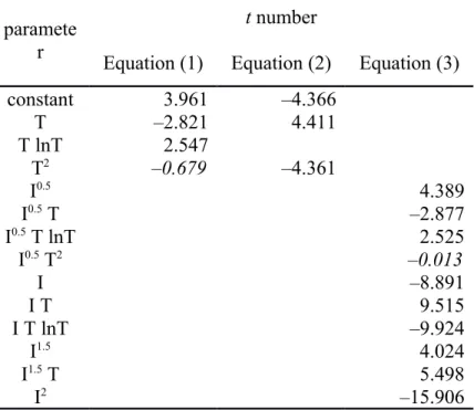
Table S2. The t number from the Regression output of the individual fitted coefficients of equations (1) to (3). The t number is the ratio of the coefficient value to its standard error and its absolute value has a Student’s t distribution. Values in italics indicate less than 95% confidence level for the significance of the coefficient.
paramete r
t number
Equation (1) Equation (2) Equation (3)
constant 3.961 –4.366
T –2.821 4.411
T lnT 2.547
T2 –0.679 –4.361
I0.5 4.389
I0.5 T –2.877
I0.5 T lnT 2.525
I0.5 T2 –0.013
I –8.891
I T 9.515
I T lnT –9.924
I1.5 4.024
I1.5 T 5.498
I2 –15.906
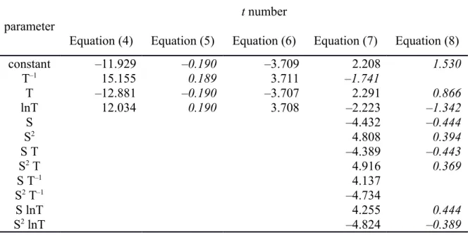
Table S3. The t number from the Regression output of the individual fitted coefficients of equations (4) to (8). The t number is the ratio of the coefficient value to its standard error and its absolute value has a Student’s t distribution. Values in italics indicate less than 95% confidence level for the significance of the coefficient.
parameter
t number
Equation (4) Equation (5) Equation (6) Equation (7) Equation (8)
constant –11.929 –0.190 –3.709 2.208 1.530
T–1 15.155 0.189 3.711 –1.741
T –12.881 –0.190 –3.707 2.291 0.866
lnT 12.034 0.190 3.708 –2.223 –1.342
S –4.432 –0.444
S2 4.808 0.394
S T –4.389 –0.443
S2 T 4.916 0.369
S T–1 4.137
S2 T–1 –4.734
S lnT 4.255 0.444
S2 lnT –4.824 –0.389
Figure S1. Residuals in as a function of temperature. The residuals are between the experimental values and fitted values (a) from equation (1) for seawater (S = 35) and temperatures from 55 to –1.7 °C, and (b) from equation (2) for seawater and brines at their freezing point. The experimental values are from Table 2 in this study (+), from Table 3 in Dickson (1990b) (○), and from Table 3 in Campbell et al. (1993) (□). Note the difference in the temperature scale of the x-axis between panels (a) and (b).
Figure S2. Residuals in pHTris (in mol on the total proton scale) as a function of temperature. The residuals are between the experimental values and fitted values (a) from