Application of numerical continuation to compute all solutions of semilinear elliptic equations
Eugene Allgower, Stefan-Gicu Cruceanu and Simon Tavener
(Communicated by A. Sommese)
Abstract. We adapt numerical continuation methods to computeallsolutions of finite difference discretizations of nonlinear boundary value problems involving the Laplacian in two dimensions.
New solutions on finer meshes are obtained from solutions on coarser meshes using a complex homotopy deformation. Two difficulties arise. First, the number of solutions typically grows with the number of mesh points and some form of filtering becomes necessary. Secondly, bifurcations may occur along homotopy paths of solutions and efficient methods to swap branches are developed when the mappings are analytic. For polynomial nonlinearities we generalize an earlier strategy for finding all solutions of two-point boundary value problems in one dimension and then introduce exclusion algorithms to extend the method to general nonlinearities.
1 Introduction
This article addresses the problem of numerically approximatingallthe solutions of a class of nonlinear second order semilinear elliptic boundary value problems with Dirichlet boundary conditions on a rectangular domain. It has been noted, see e.g. [6], that there are very few theoretical results concerning how many solutions such a problem may have, or indeed, if there are any solutions at all. This state of affairs is somewhat better in the corresponding case of second order ordinary differential equations, where a number of existence and multiplicity results are available in several papers and books, see, e.g., the references in [3]. The approach taken here is to perform a standard finite difference approximation of the partial derivatives and then to numerically seek all of the solutions to the resulting nonlinear systems of equations. This approach worked very successfully for ordinary differential equations when the nonlinearities were of polynomial type [3].
The example considered in [3] was
u′′=f(x, u, u′)
with general linear boundary conditions andf assumed to be a polynomial map in theu- variable. For this case, the totality of solutions of the polynomial systems of equations was
found by embedding the systems in a complex setting and applying a numerical homotopy continuation method to compute all of the complex solutions of the polynomial system.
There are some drawbacks however, which need to be addressed. One of them is that the requirement for an accurate discretization can result in a very large polynomial system and therefore an enormous number of complex solutions, among which are only a few real solutions that are actually of interest. To illustrate this point, let us mention the familiar theorem of Bezout [13, 8, 14], which essentially states that the number of (finite) complex solutions, accounting for multiplicities, can be as much as the product of the degrees of each of the equations. So, for example,Nquadratic equations would generally have 2N solutions in CN. Furthermore, even among the real solutions, there may be spurious solutions which arise as numerical artifacts and do not converge to solutions of the boundary value problem.
The above drawbacks were treated in [3] for two point boundary value problems by means of two remedial steps. The first step was to discard the obviously irrelevant so- lutions, including the real solutions which did not exhibit properties which theoretical results showed must hold, for example, symmetry properties. The second remedy was to start with a crude mesh (and hence a low dimensional system) and then to introduce a new mesh point via a continuous deformation of the mesh. Assuming that the solutions had been obtained for a uniform mesh with, sayN points, a new point was introduced, for example, at the right boundary and this point was then allowed to be continuously moved leftward until a uniform mesh with(N+1)points was achieved. This device was suggested in [2] and implemented in [3]. It uses numerical continuation in yet another way since the homotopy parameter now is used to continuously deform the mesh in the difference equations. Starting points for solutions when the new point is introduced are simply the zero points of a single polynomial equation, which are generally easy to find.
For example, one may apply an algorithm for finding the eigenvalues of the corresponding companion matrix.
In essence, it would seem straightforward to extend the ideas used in [3] to a cor- responding case of partial differential equations in two dimensions. Let us take as our paradigm the equation
∆u=f(x, y, u, ux, uy) onΩ⊂R2, u=g on∂Ω,
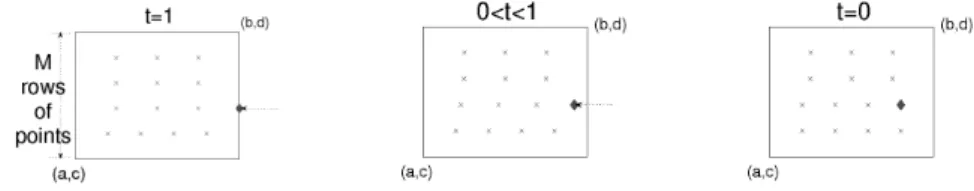
wheref is assumed to be an analytic map. One new issue which needs to be confronted is that of introducing mesh points in a manner which does not require a large number of new points, due to the fact that the number of solutions would grow too rapidly. Such a moving mesh is described in Section 3.4. The approach proceeds as follows. Suppose that the solutions have been found for a uniform square mesh in the square domain. In a fashion as described in the previous paragraph, a new point is introduced at the right boundary of the first row of mesh points and is allowed to move leftward until the points in the first row are again equally spaced. The same process is repeated for each of the rows and then for each of the columns, this time by introducing a point at the top of each column until once again a uniform square mesh is attained. The entire procedure requires a careful handling of the underlying stiffness matrices for the moving meshes. Now however, the
resulting meshes do not generally exhibit symmetries even at termination of introducing the moving mesh-point. Symmetry conditions for discarding spurious solutions need to be correspondingly modified.
Bifurcation can occur along the homotopy paths. For the class of problems being considered here, the homotopy paths are the solutions of a system of equations of the formH(t, z) = 0 whereH : [0,1]×Cn → Cn is analytic in the z-variables. We have shown in [4] that in the above analytic setting any turning point of a homotopy path is necessarily also a bifurcation point and that the bifurcating directions are orthogonal.
Thus the tangent vectors at the bifurcation point are orthogonal and switching solution paths on to the new bifurcating branch at such points is easily accomplished.
McKenna and Plum [6] study a particular boundary value problem involving a quadra- tic nonlinearity on a square domain and prove that at least four solutions exist for a par- ticular value of a parameter arising in the equation. They conjecture the form of the bifurcation diagram and suggest that more than four solutions may occur as the parameter is increased. We apply our techniques to this problem in Section 4.3, where we confirm the bifurcation diagram and demonstrate that no more than four solutions occur over a large positive range of the parameter values.
In Section 5, a generalization is made which allows non-polynomial nonlinearities in the partial differential equation. In the polynomial case when a new mesh point was introduced, the starting solutions were obtained as the eigenvalues of the corresponding companion matrix. For non-polynomial nonlinearities there may be infinitely many com- plex solutions and it is necessary to seek solutions in a bounded region which is taken to be a rectangle inC. The real solutions are then found by means of a cellular exclusion algorithm. Cellular exclusion algorithms have recently been studied by several authors, see e.g. [9] and the references there. With cellular exclusion methods, all real solutions to nonlinear systems of equations within a rectangularn-cell can be found, provided the nonlinearity satisfies some rather mild conditions, such as Lipschitz conditions on the components. On the other hand, if the nonlinearity has a Taylor expansion, the efficiency of the exclusion algorithm can be significantly improved. This approach is applied to the familiar Bratu equation in one dimension.
The present study has been restricted to a special, but familiar class of boundary value problems mainly to illustrate the effectiveness of the techniques presented. It should be emphasized that the methods presented here are not meant to provide fast and accurate methods for solving partial differential equations. Rather, the idea is to glean reliable in- formation concerning the number and qualitative properties of solutions. The approxima- tions which are obtained may however be used as starting values to obtain more accurate solutions on much finer meshes.
2 Homotopy continuation for ODEs
In this section we briefly review the approach used in [3] for numerically finding all solutions to two-point boundary value problems. Consider the second order boundary
value problem on the interval[a, b]⊂R
u′′=f(x, u, u′), (1)
with the boundary conditionsu(a) =αandu(b) =β. Using a central difference approx- imation with a uniform mesh for example, we can approximate a solutionu(x)of (1) by anN-tuple of numbers(u1, u2, . . . , uN)T such thatui ≈u(xi)fori=1, . . . , N, where we seth := N+1b−a,xi :=a+ihfori = 0, . . . , N +1,u0 =α, anduN+1 =β. The discretization of (1) takes the form of the following systemDN,
DN
u0 − 2u1 + u2 = h2f x1, u1,u22h−u0 ,
... ... ... = ...
uN−1 − 2uN + uN+1 = h2f xN, uN,uN+12h−uN−1 . We are seeking all the real solutions of (1) and we know that depending upon the right hand sidef, Equation (1) may have no solution, a unique solution, multiple solutions, or even infinitely many solutions. There are several theorems that state sufficient conditions for the existence of solutions for such equations, but even when the existence is known, the number of solutions is often not. In [3], the authors studied a relatively secure numerical technique for finding all the solutions for such an equation in the case thatf(x, u, u′) is a polynomial depending onu. The idea is to complexify the problem and find all the solutions (real and complex) of an associated polynomial systemPN(z)using a homotopy function which will track some known starting solutions to all the solutions ofPN(z). A drawback of this approach is that the number of solutions ofPN(z)can be quite large (as is known from Bezout’s theorem) and hence sifting out solutions which are irrelevant to (1) becomes a significant issue.
The process of finding the solutions can be sketched in four steps.
1. Find all the solutions of the discretizationDN for some smallN.
2. Discard all unreasonable solutions and denote bySNthe set of the solutions which are kept.
3. If the mesh size is not sufficiently small or the cardinality ofSNhas not yet stabilized, then add a mesh point to obtain the discretizationDN+1. Use the solutions inSN to generate solutions ofDN+1and then return to step 2 to generateSN+1.
4. Once the mesh size is sufficiently small and the cardinality ofSN becomes stable, refine the solutions to a more consistent grid with a fast nonlinear solver.
As one can imagine, the key step in this process is step 3. To solve this, we build a homotopy function such as the following, which produces a mesh refinement as a result of a continuous deformation.
LetHN+1(u1, u2, . . . , uN+1, t) :=
u0−2u1+u2 − h(t)2f x1(t), u1,u2h(t)2−u0 ...
uN−2−2uN−1+uN − h(t)2f xN−1(t), uN−1,uN2h(t)−uN−2 uN−1−2uN +UN+1(t) − h(t)2f xN(t), uN,UN+12h(t)(t)−uN−1 uN−2uN+1+UN+2(t) − h(t)2f xN+1(t), uN+1,UN+22h(t)(t)−uN
(2)
with
xi(t) =a+ih(t), fori=1, . . . , N+1, u0 =α,
h(t) =t Nb−a+1
+ (1−t) N+2b−a , UN+1(t) = (1−t)uN+1+βt, UN+2(t) =β(1−t).
(3)
Remark 2.1. (a) Att=0,HN+1represents the systemDN+1.
(b) Att = 1,HN+1 can be interpreted as the systemDN with a new mesh point hav- ing the valueuN+1 atxN+1 = band a new right-hand boundary having the value UN+2(1) =0 atxN+2=b+h(1).
(c) There is an incompatibility between the old boundary condition at x = b and the new one atx =b+h(1), but this is accommodated by the presence of bothuN+1
andUN+1, which are not necessarily equal. Astgoes from 1 to 0, the mesh points are squeezed back inside of[a, b]and right hand boundary condition u(b) = β is transferred fromUN+1toUN+2asUN+1is enforced to equaluN+1, i.e.,
UN+2(0) =β and UN+1(0) =uN+1.
To find all the solutions ofDN+1, we will use numerical continuation to track the zeros ofHN+1astgoes from 1 to 0. Att=1, we have a listSN of solutions(u1, u2, . . . , uN)T satisfying the firstN equations ofHN+1, while the final equation is
uN −2uN+1=h(1)2f
b, uN+1, −uN
2h(1)
, (4)
which is the only place whereuN+1appears. For each solution(u1, u2, . . . , uN)T inSN, we use this equation to find the corresponding values ofuN+1. These are the starting points of continuation paths leading to solutions ofDN+1.
Remark 2.2. This framework will not change in any of its essentials if we prescribe in (3) a different function forUN+2(for example, the constant functionUN+2=β).The essential feature ofUN+2is that it goes toβastgoes from1to0.
Remark 2.3. In the case of polynomial nonlinearity whenf(x, u, u′)from (1) is a real polynomialp(u), we can conveniently obtain the starting points forHN+1(u1, u2, . . . , uN+1,1) =0 by solving the polynomial equation
uN −2uN+1+UN+2(1)−b−a N+1
2
p(uN+1) =0, (5) foruN+1givenuN from the solutions inSN. All the solutions (real and complex) of (5) can be found using standard available software. For small degree polynomials, the com- panion matrix may be used to find these zeros.
If we denote d = degp(u), then one can see that over the complex numbers we obtaindvalues ofuN+1for every solution inSN. If we suppose that at each stage of the algorithm these will continue to finite, nonsingular solutions ofDN+1, thenSN will have dN entries. Therefore, the number of the solutions forDN+1 grows exponentially asN increases, and hence the need of some filters becomes very important.
Next, we will extend the concept to two-dimensional partial differential equations and to non-polynomial right hand sides.
3 Homotopy continuation for two-dimensional PDEs
The method of finding all the solutions of second order ordinary differential equations presented in the previous section is now generalized to a class of nonlinear second or- der semilinear elliptic boundary value problems with Dirichlet boundary conditions on a rectangular domain, but still with polynomial nonlinearities. Most of the difficulties met for the one-dimensional case are also encountered in the new type of problems. Further difficulties that appear due to the generalization to a higher dimension are described in the first part of this section.
We build a homotopy function associated with a central difference discretization of the Laplace operator as a combination of some sparse matrices and vectors. All calculations necessary when introducing a new mesh point into a row are provided. The calculations necessary when introducing a new mesh point into a column are similar and are not pre- sented. Both cases were implemented since we introduced mesh points into rows and columns alternately. The geometry of the moving mesh-grid is presented in Section 3.2.1.
3.1 Difficulties for ODEs and PDEs. We will concentrate on findingallthe solutions for a problem of the form
∆u=f(λ, x, y, u, ux, uy) onΩ⊂R2, u|∂Ω=g,
whereΩis a rectangular domain. In the next sections we will develop a method to solve this problem numerically. Before doing so, we review some difficulties that arose in the one-dimensional case.
3.1.1 Exponential growth of the number of the solutions. In the case of a polynomial nonlinearity, the number of complex solutions grows exponentially with the number of interior mesh points. We stop the computation with a heuristic criterion, e.g., when a desired number of interior mesh points has been attained, or the number of real solutions has stabilized, or the number of real solutions is growing without bound. In all the one- dimensional problems that we have examined, the number of real solutions stabilized or grew without bound. Once this was determined, we were able to take these solutions with 6–7 interior points and refine them to a finer grid. Supposing that 6–7 interior points for a one-dimensional interval will be satisfactory (providing that the number of real solutions
stabilizes or grows without bound), then for a two-dimensional problem on a rectangular domain we would be satisfied with 36–49 interior points. Clearly so many mesh points will lead to a great number of solutions for the homotopy and this will require stricter tests for filtering out unwanted solutions. For the one-dimensional case, properties off to conclude symmetries of solutions were used as a filter in [3]. In higher dimensions it becomes more critical to filter out spurious solutions.
3.1.2 Turning points and bifurcations. An issue of concern arising in homotopy methods is the possibility that singular points such as turning points and bifurcation points may occur on the homotopy paths. One remedy is to introduce a random perturbation into the system, as for example, in the “Γ-trick” as discussed in [3]. While multiple solutions are relatively rare in the discretizations of boundary value problems for ODE’s, they arise regularly for PDE’s in the presence of solutions which are symmetric under groups of rota- tion and reflection transformations. For these reasons we have used continuation methods which incorporate arclength parametrization and easily round turning points. Arclength parametrization for analytic homotopy maps was examined in [4, 7] where it was shown that simple turning points in the homotopy parameter are also the site of simple bifurca- tion points, as defined below. We summarize here the results which enable a monotone tracing of homotopy paths.
Definition 3.1.1(Simple turning point). LetH : Rn+1 → Rn be sufficiently smooth.
Suppose thatc : J →Rn+1,c(s) = (t(s), u(s))is a smooth curve, defined on an open intervalJ, and parametrized (for reasons of simplicity) with respect to arclength such that H(c(s)) =0 fors∈J. The pointc(¯s)is said to be a simple turning point of the equation H=0 ift(¯˙s) =0,¨t(¯s)6=0, and the Jacobian
t˙ u˙ Ht Hu
c(¯s)
has minimum rank deficiency.
Definition 3.1.2(Simple bifurcation point). Let H : Rn+1 → Rn be a sufficiently smooth map. A pointu¯ ∈ Rn+1 is called a simple bifurcation point of the equation H=0 if the following conditions hold,
(1) H(¯u) =0,
(2) dim kerH′(¯u) =2,
(3) e⋆H′′(¯u)[φ, ψ]has one positive and one negative eigenvalue, where the vectorespans kerH′(¯u)⋆ andφandψtogether span kerH′(¯u), whereH′′(¯u)[φ, ψ] is a bilinear form acting on the vectorsφandψ.
Now, letH :R×Cn→Cnbe a smooth homotopy. Assume thatH(t, w)is analytic in the variablesw. We will also writew=u+ivforw∈Cn, whereu, v ∈Rndenote the real and the imaginary parts ofwrespectively. Note thatH(t, w) =H(t, w)sinceH is analytic. Let us define now the real and imaginary partsHr, Hi:R×Rn×Rn→Rn
by
Hr(t, u, v) =1
2(H(t, w) +H(t, w)), Hi(t, u, v) =−i
2 (H(t, w)−H(t, w)),
(6)
and the mapHˆ :R×Rn×Rn→R2nby H(t, u, v) =ˆ
Hr(t, u, v)
−Hi(t, u, v)
. (7)
Theorem 3.1.3. Letˆc(s) = (t(s), u(s), v(s))be a solution curve ofHˆ−1(0). Any simple turning pointc(¯ˆs)of the equationHˆ =0is also a simple bifurcation point of the same equation.
Theorem 3.1.4. Under the assumptions of Theorem3.1.3, let us now denote the two bi- furcating solution curves ofHˆ−1(0) byˆci(s) = (ti(s), ui(s), vi(s)),i ∈ {1,2}. The curves are defined forsnears¯andc˜= ˆc1(¯s) = ˆc2(¯s)is the bifurcation point. Then
(i) (0,u˙1(¯s),v˙1(¯s))and (0,−v˙1(¯s),u˙1(¯s))are orthogonal unit tangents toˆc1(s)and ˆ
c2(s)ats= ¯s, respectively, (ii) ¨t1(¯s) =−t¨2(¯s).
Remark 3.1.5. The above theorems generalize Propositions 11.8.10 and 11.8.16 in [5].
The proofs are similar in concept and may be seen in [4] which is available as a preprint athttp://www.math.colostate.edu/∼tavener/.
Remark 3.1.6. Theorem 3.1.3 shows that bifurcation points can be detected by noting turning points along the homotopy path. Turning points are easily detected by, for ex- ample, monitoring whether the inner product of successive unit tangent vectors becomes negative. Most numerical implementations of continuation methods construct tangent
“predictor” vectors as points along the branch are calculated. Theorem 3.1.4 shows that one can easily change branches because the appropriate “predictor” vector for the bifur- cating branch is orthogonal to the tangents of the solution curve near the bifurcation point.
In this way, one can can trace homotopy paths monotonically astdecreases to 0.
3.2 Implementation details.
3.2.1 Details on the two-dimensional grid for∆u=f(λ, x, y, u, ux, uy). In this section we use numerical continuation to find all the solutions for a problem of the form
∆u=f(λ, x, y, u, ux, uy) onΩ = [a, b]×[c, d]⊂R2, (8)
u=g on∂Ω. (9)
Using a standard central difference approximation, with a uniform mesh withN inte- rior points, the discretization of (8, 9) takes the form
DN : Axx~u+~bxx+Ayy~u+~byy =f~ (10)
where~u = (u1, u2, . . . , uN)T is the discretized solution vector of the unknowns. Here, the discretization for∂∂x2u2 incorporating the left and right boundary conditions isAxx~u+
~bxx. The discretization for ∂∂y2u2 incorporating the upper and lower boundary conditions is Ayy~u+~byy.
As in the one-dimensional case, we will continue introducingonepoint at a time since introducing a row or column ofppoints would require solving a system ofppolynomial equations to find the starting solutions for our homotopy. Introducing new mesh points one at a time also allows us to filter more frequently.
3.2.2 The homotopy function for ∆u = f(λ, x, y, u, ux, uy). We rewrite the boundary value problem (8, 9) as
∆u=f(λ, x, y, u, ux, uy) onΩ = [a, b]×[c, d]⊂R2, (11) u|x=a=ua(x), u|x=b=ub(x), u|y=c=uc(y), u|y=d=ud(y). (12) The main obstacle to be overcome when introducing extra points one at a time is the approximation of the Laplacian on non-regular finite difference meshes. This is achieved by appropriate application of linear interpolation. Details regarding the approximation of the derivatives for the general case of introducing a mesh point are given in Appendix A.
Figure 1. Introducing a new point()in the 2ndrow.
As indicated in (10), the boundary value problem (11, 12) can be discretized as Axx~u+~bxx+Ayy~u+~byy =f ,~
whereA=Axx+Ayyis the stiffness matrix and~bxx,~byyare what we will call bound- ary vectors. The corresponding homotopy (2) for this two-dimensional boundary value problem is
HN(~u, t) := (Axx+Ayy)~u+ (~bxx+~byy)−f ,~ (13) where the explicit forms forAxx,Ayy,~bxx,~byy, andf~are given in Appendix B.
3.3 Stopping strategies. Independently of the details of the method we use to track the solutions of the homotopyHN fromt =1 tot =0, we must land exactly ont =0 because only at t = 0 does the incompatibility between the old boundary conditions and the new ones disappear (see Remark 2.1 for more details). We have two stopping strategies.
i) As we track a solution, the homotopy parameter t will decrease from 1 toward 0.
Whentis very close to 0, we choose the final steplength such thattis precisely 0.
Using this method,twill always stay in the interval[0,1].
ii) We track a solution path untiltbecomes negative for the first time. We then choose a “backward” steplength such thattlands precisely on 0.
The disadvantage of the second strategy is that we require an extra step to land on t =0. This however is insignificant in comparison with the advantage that any turning point near t = 0 will be observed and the switch to the proper branch as suggested in Remark 3.1.6 can be performed. Some of the possible paths that can be met in the tracking process are presented in Figure 2.
Figure 2. Possible paths in the tracking process.
3.4 Algorithm for the moving mesh. Let us describe the steps for finding all solutions to
∆u=f(u) on Ω = [0,1]×[0,1], u=0 on ∂Ω.
Let us use the finite difference discretization as described in Appendix B and form the homotopy map as in Equation (13). Letl be the number of the row or column to which a mesh point is introduced in a continuous manner ast goes fromt =1 tot = 0. Let N be the current number of mesh points. Fort =1, the solutions toHN(¯u,1) =0 are available from the previous solution. For example, iff is a polynomial, the solutions toHN(¯u,0) = 0 are found by finding the eigenvalues of the corresponding companion matrix of HN(¯u,0). Similarly, at the introduction of a new mesh point on a row or column, the starting points for the homotopy are also found by solving a single polynomial equation in thelthequation.
Algorithm 1Mesh refinement procedure SolveH1(¯u,0) =0 (companion matrix) forM =1 toMmaxdo
{Add mesh points to rows} forl=1 toM do
N =M2+l
Find all solutionss, such that¯ HN(¯s,1) =0 (companion matrix)
For all solutions¯s, traceHN(¯u, t) =0 withHN(¯s,1) =0 to obtain all solutions
¯
uwithHN(¯u,0) =0 (homotopy)
Delete spurious solutions to obtain a setSN
end for
{Add mesh points to columns} forl=1 toM +1do
N =M2+M +l
Find all solutionss, such that¯ HN(¯s,1) =0 (companion matrix)
For all solutions¯s, traceHN(¯u, t) =0 withHN(¯s,1) =0 to obtain all solutions
¯
uwithHN(¯u,0) =0 (homotopy)
Delete spurious solutions to obtain a setSN
end for end for
Remark 3.4.1. EitherMmaxis chosen at the outset or one can stop when the number of solutions inSN has become constant. The homotopy tracking incorporates the tests for turning points and branch switching as outlined above.
4 Numerical results for polynomial right hand side
4.1 Numerical results for∆u=−(1+u2). We now consider the following partial differential equation in two dimensions,
∆u=−(1+u2) onΩ = [0,1]×[0,1], (14)
u=0 on∂Ω. (15)
Using a tracking method based on arclength continuation and the techniques presented in Section 3 we obtained the results in Table 1. In particular, we switched branches at turning points as discussed in Remark 3.1.6.
In every case, the starting points for the homotopies were the solutions from the pre- vious mesh. A solution is considered to be real if the magnitude of the imaginary part at each mesh point was less than 10−8. For eachN =1, . . . ,16 interior points, we have ob- tained exactly the maximum possible number of solutions indicated by Bezout’s theorem.
Out of these, the number of real solutions stabilized to 2 asN increased.
Remark 4.1.1. Our implementation of numerical continuation used steplength controls as suggested in [5]. In particular, the residuals of predictors, angles between successive
N l r/c No. No. real Solutions with same The value oftat solutions solutions turning points the turning points
1 1 r 2 2
2 1 r 4 2
3 1 c 8 2 (5,7) 0.1003
4 2 c 16 2 (11,15) 0.0036
(18,16) 0.9245
5 1 r 32 6 (2,10) 0.8573
(23,31) 0.3553
(47,51) 0.9831
6 2 r 64 4 (48,52) 0.9438
(3,19) 0.9242
(35,63) 0.3592
(7,39) 0.9739
7 1 c 128 4 (8,72) 0.8996 & 0.0175
(71,127) 0.3853
(79,143) 0.9970
8 2 c 256 4 (80,144) 0.9616
(15,255) 0.4410
9 3 c 512 2 (31,511) 0.3820
10 1 r 1024 2 (63,1023) 0.4828
11 2 r 2048 2 (127,2047) 0.5638
12 3 r 4096 2 (255,4095) 0.4858
13 1 c 8192 2 (511,8191) 0.4945
14 2 c 16384 2 (1023,16383) 0.5907
15 3 c 32768 2 (2047,32767) 0.5920
16 4 c 65536 2 (4095,65535) 0.4985
Table 1. The number of solutions for∆u=−(1+u2)onΩ = [0,1]×[0,1]with zero Dirichlet boundary conditions.
tangents and empirical monitoring of the contraction rate of corrector steps were incor- porated. Thus we were able to resolve turning points which were very close tot=1 and t=0 successfully. Without such care we would perhaps not have noted the turning points att=0.0036 andt=0.9970 forN =4 andN =8 interior points, respectively.
Remark 4.1.2. In this example, as in fact in all the ones we studied, during our tracking we met all the possible paths presented in Figure 2, except the one denotedγ. A path with exactly two turning points as portrayed byδoccurred atN =7 interior points.
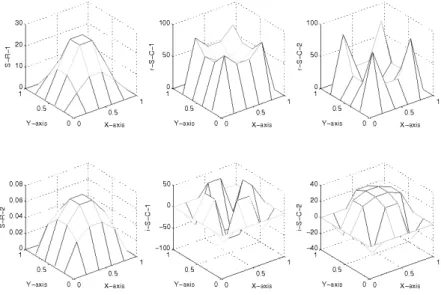
Of those 216solutions for 16 interior points, there were exactly two real and four com- plex ones which are invariant under the dihedral groupD4of symmetries of the square. In Figure 3 we have plotted these six solutions with 4×4 interior points. Using interpolation of these as initial guesses for Newton iterations, we have obtained the refined solutions plotted in Figure 4. S-R-1 and S-R-2 are the two real solutions, r-S-C-1 and i-S-C-1 are the real and the imaginary parts respectively of one of the four complex solutions, r-S-C-2 and i-S-C-2 are the real and the imaginary parts respectively of another of the four com- plex solutions. The other two complex solutions are the conjugate of S-C-1 and S-C-2.
Only these six solutions did not undergo significant modifications as we refined the grid.
4.2 Numerical results for∆u = −λ(1+u2). The bifurcation diagram for∆u=
−λ(1+u2)with zero Dirichlet boundary conditions was independently produced using an arclength continuation algorithm on a 39×39 mesh. Here, and elsewhere in this paper, we obtained bifurcation diagrams by plotting the infinity norm of the solutions versus the
Figure 3. Six solutions for∆u=−(1+u2)with 4×4 interior points.
Figure 4. The six solutions for∆u=−(1+u2)refined to 39×39 interior points.
Figure 5. The bifurcation diagram for∆u=−λ(1+u2)with zero Dirichlet boundary conditions.
parameterλ. Two turning points are attained at±λ⋆, whereλ⋆ =9.1890. The two real solutions shown in Figure 4 correspond to the two intersections of the bifurcation diagram with a vertical line drawn atλ=1. Forλ=10, our mesh deformation method produced no real solutions out of 2N complex ones. Forλ=9 (a value close to the turning point λ⋆ =9.1890), we found no real solutions for the first 4 interior points. One real solution appeared after introducing the 5th interior point. The second real solution appeared only after introducing many more interior points. For values of 9< λ < λ⋆the real solutions appeared only after introducing more than 5 interior points. Our results also indicate there are no disjoint branches in the bifurcation diagram.
4.3 The problem of Breuer, McKenna and Plum. We used the methods described in the previous section to examine a conjecture posed in [6] where the following theorem was provided.
Theorem 4.3.1. The equation
∆u+u2=800sinπxsinπy inΩ, u=0 on∂Ω (16) whereΩ = (0,1)×(0,1), has at least four solutions.
Our approach will give all the solutions of (8) not only forf(u)being a polynomial ofu, but also for any functionf(x, y, u)that is a polynomial as a function ofu, because even in this case, the equation corresponding to (5) for our two-dimensional BVP is still a polynomial equation in one unknown. For problem (16), we found using our homo- topy continuation that there are exactly four real solutions which are essentially different.
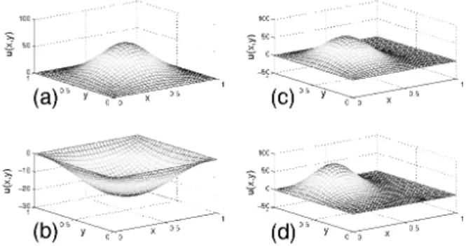
We also got real solutions that are rotations or reflections of these, but after filtering to remove these conjugate solutions, we obtained only the four truly distinct real solutions that appear in Figure 6.
Figure 6. The four real solutions for (16).
The solutions (a) and (b) are fully symmetric (i.e., symmetric with respect to reflec- tions about the axesx= 12,y= 12,x=y, andx=1−y), the solution (c) is symmetric only with respect to reflection abouty = 12, and the solution (d) is symmetric only with respect to reflection aboutx+y=0.
The peaks of the positive and negative fully symmetric solutions (a) and (b) are 61.776 and−21.358, respectively. The peak of the solution (c) has the value 69.923 and is attained at(x, y) ≈ (165,12). The peak of the solution (d) has the value 76.321 and is attained at(x, y) ≈ (13,23). All these values were found using a mesh with 63×63 interior points.
A generalization of Equation (16) considered in [6] is
∆u+u2=λsinπxsinπy inΩ, u=0 on∂Ω. (17)
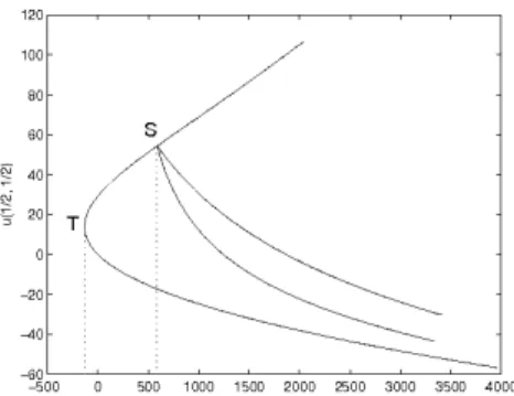
Starting with the 4 solutions found forλ = 800 on a mesh with 31×31 interior points, we used arclength numerical continuation to construct the bifurcation diagram in Figure 7.
Figure 7. The bifurcation diagram for (16).
We found a turning pointT atλT ≈ −133.3 at which one eigenvalue of the Jacobian changes sign. The Jacobian is in factA+2diag(~u), where A is the stiffness matrix (see Section 3.2.2). We also found a symmetry breaking bifurcationS atλS ≈ 587.7 at which a pair of other eigenvalues of the Jacobian (a double eigenvalue) changes sign.
We performed continuation for values ofλup to 8000 and saw no indication that another eigenvalue will approach zero asλincreases.
In order to test our findings, we performed homotopy continuation for a few different values ofλand confirmed that there are no real solutions forλ < λT, two real solutions ifλT < λ < λS, and four real solutions ifλ > λS. Furthermore, we confirmed that there do not seem to be disjoint real branches in this bifurcation diagram.
Breuer, McKenna and Plum review several natural conjectures which may be made for equations such as (17). Two such conjectures are, (i) asλ → ∞there are at least four solutions (weak version) and, (ii) more solutions are created as bifurcations from the positive curve, considerably further up the positive branch (the stronger version). Using a Mountain Pass Algorithm, Breuer, McKenna and Plum find the weak conjecture is true, but the strong one seems to be false. This coincides with our results.
5 Homotopy continuation for nonpolynomial nonlinearity
We now generalize our method to nonpolynomial nonlinearities in the partial differential problems. The algorithm described in Section 2 works well for the case when the function f is a polynomial inu, because in this case, by using companion matrices we are able to findallthe solutions of the polynomial Equation (4) that resulted from the introduction of a new mesh point. When the nonlinearityf is not a polynomial, there is no general method to find all solutions.
Indeed, solving Equation (4) now becomes quite different. For example, it may have no solutions at all, even under complexification. In this case, we may conclude that the corresponding boundary value problem also has no solutions. Another possibility is that (4) may have infinitely many solutions, particularly when the complexification is considered. Since it is not feasible to compute infinitely many solutions, it becomes nec- essary to confine the search for solutions to some compact region (such as a rectangle in C, or correspondingly inR2). The choice of the rectangle may be predicted based upon a priori estimates or on some practical bound on the norm of the solutions.
The Bratu problem considered in the next section illustrates how matters differ from the polynomial case, but also the necessity to use the complexification of (4). Since we now seekallthe solutions to (4) in a bounded domain and under weakened assumptions onf, we are led to consider cellular exclusion methods. We briefly introduce the concept in Section 5.2.
5.1 The Bratu problem and the exclusion method. The toolbox developed in [3] was used to find all the solutions of a one-dimensional boundary value problem of the form
u′′=f(x, u, u′), x∈(a, b), u(a) =α, u(b) =β
wheref is a polynomial ofu. We now consider the case in whichf is not a polynomial function ofu. As an example, we will look at the one-dimensional Bratu Problem
u′′+λexp(u) =0 on(0,1),
u(0) =u(1) =0. (18)
Let us associate the homotopy function from (2) and (3) to this problem. To be able to use our algorithm for finding all the solutions of (18) for a specific value ofλ, we need to be able to find all the roots of the Equation (4) which, for this case, can be rewritten as
uN−2uN+1+λ 1 N+1
2
exp(uN+1) =0. (19) Therefore we now have to find all the real solutions of the equation
exp(u)−au+b=0, (20)
whereaandbare positive constants,a =2(N +1)2/λ,b =uN(N +1)2/λ. One can easily see that the number of real zeros for such an equation is either 2, 1 or 0, depending upon whethera(1−ln(a)) +bis negative, zero or positive, respectively. One can also easily implement a method to find the real zeros of this equation and integrate that into our homotopy continuation approach (it might help to see thatb/ais a lower bound for these zeros, if they exist).
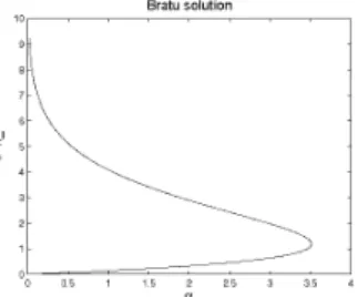
For everyλ∈[0,2.1]which we tried, we obtained only two real solutions every time we introduced a new grid point. It is well known that the Bratu problem has two real solutions forλ∈[0, λ∗], whereλ∗ ≈3.5127 represents the value of the turning point in the bifurcation diagram from Figure 8.
Figure 8. The bifurcation diagram for the Bratu Problem.
In the interval [2.1, λ∗] the difficulty we encountered was the fact that the Equa- tion (20) did not have anyrealzeros for small numbers of mesh points, and therefore we could not start using our homotopy. This reminds us of a fact encountered in the poly- nomial case, that sometimes real solutions will arise from complex ones as we increase the number of interior points. Therefore, it is not sufficient to know how to solve (20) only for real solutions, but also for the complex ones.
Writingu=uℜ+iuℑandb=bℜ+ibℑ, Equation (20) now takes the form exp(uℜ) cos(uℑ)−auℜ+bℜ=0
exp(uℜ) sin(uℑ)−auℑ+bℑ=0. (21) The necessity of solving this system for the real variablesuℜanduℑled us to consider the exclusion algorithms. Using these algorithms, we were able to find all the solutions uℜanduℑof this system in a rectangle.
5.2 Exclusion algorithm. In this section we will give some background about the ex- clusion algorithms that we will use here (see also [9]). Exclusion methods provide a useful tool for finding all the solutions of a nonlinear system of equations over a compact domain. They may also be used for finding the global minima of a function. The concept goes back to Moore [12]. Further research on cellular exclusion algorithms to find all the solutions of a nonlinear system appears in [17, 16, 15, 11]. Georg and collaborators [9, 1, 10] introduced and analyzed several new tests for finding the zeros and the global minima of functions over a compact domain. The results led to significant improvements in the efficiency of the methods.
In Rn andRm×n we use the component-wise “≤” as a partial ordering, “| · |” as the component-wise absolute value, and “k · k∞” as the max norm. For example, for two matricesA, B ∈ Rm×n, the symbolA ≤B means thatA(i, j) ≤B(i, j)fori = 1, . . . , m,j=1, . . . , n.
Definition 5.2.1. An intervalσinRnis a compact cell of the form
σ= [mσ−rσ, mσ+rσ] ={x∈Rn:mσ−rσ ≤x≤mσ+rσ},
wheremσ, rσ∈Rnare called the midpoint and the radius ofσrespectively, withrσ(i)>
0 fori=1, . . . , n. Also,mσ−rσandmσ+rσare called the lower and upper corners respectively.
Definition 5.2.2(Exclusion test). Let σ ∈ Rn be an interval and F : σ → Rn be a function defined onσ. A test
TF(σ)∈ {0,1} where 0≡no and 1≡yes
is called an exclusion test forFonσiffTF(σ) =0 implies thatFhas no zero point inσ.
Therefore,TF(σ) =1 is a necessary condition forF to have a zero point inσ.
Example 5.2.3. LetL >0 be a Lipschitz constant forf on the intervalσ. Then
f(mσ)≤Lkrσk (22)
is an exclusion test forfonσ.
If an exclusion test is given (assuming thatTF(σ)is available for any subintervalσ of some initial intervalΛon whichFis defined), then we can recursively bisect intervals and discard the ones which yield a negative test. This is the basic idea of an Exclusion Algorithm.
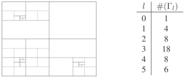
We use a strategy of cyclic bisections of the intervals along successive axes. We say that we have reached a new bisection level whenever one cycle of bisections is ac- complished. We also think of an exclusion algorithm as performing a fixed number of bisection levels. We will denote byΓlthe list of the intervals generated by the algorithm on thelthlevel, which are in fact the intervals that have not been discarded afterlbisection levels.
It is obvious that ifΓl =φfor some levell, then the algorithm has shown that there are no zero points ofF in the initial intervalΛ.
Algorithm 2Exclusion Algorithm Γ← {Λ}
forl=1, . . . , maximal leveldo fora=1, . . . , ndo
Γ˜ is obtained by bisecting eachσ∈Γalong the axisa forσ∈Γ˜do
ifTF(σ) =0then
dropσfromΓ˜(σis excluded) end if
end for Γ←Γ˜ end for Γl←Γ end for
The exclusion tests we discuss are applied component-wise on vector-valued function F :σ →Rn. Therefore, we only need to consider an exclusion test for a scalar-valued functionf : σ→Rand then combine such (possibly different types of) exclusion tests
l #(Γl)
0 1
1 4
2 8
3 18
4 8
5 6
Figure 9. Bisection levels for a cellσ⊂R2. The figure shows the surviving cells at levels l=0, . . . ,6.
to obtain an exclusion test for a vector-valued functionF = {fi}i=1,...,n : σ → Rn by settingTF(σ) = Qn
i=1Tfi(σ). Hence, we may concentrate our attention on scalar functionsf : σ → Rwhen designing exclusion tests. We also need good exclusion tests which are computationally inexpensive but relatively tight, because otherwise too many intervals remain undiscarded on each bisection level and this will lead to significant numerical inefficiency.
Definition 5.2.4. For two power seriesf(x) = P
αfαxα andg(x) = P
αgαxα we define
f ≺≺g ⇐⇒ |fα| ≤gαfor allα.
Some simple exclusion tests were given in [16, 15] and the following complexity result was also shown.
Theorem 5.2.5. LetΛ⊂Rnbe an interval,F : Λ→Rnand zero a regular value ofF.
Then there is a constantC > 0such that the algorithm started inΛgenerates no more thanCintervals on each bisection level, i.e.#(Γl)≤Cindependent ofl.
Remark 5.2.6. The constantCcan be very big and numerical experiments have shown that some exclusion tests ((22) for example) are not tight enough for non-linear systems in which some solutions may be singular.
5.3 Exclusion tests via dominant functions. Georg [9] gave efficient exclusion tests based on the concept of dominant functions by using Taylor expansions. He gave several results for explicitly constructing dominant functions. We now briefly review some of these ideas from that paper.
Definition 5.3.1. Letσ⊂Rnbe an interval. We denote:
Ak(σ) :={f :σ→Rn:∂αf is absolutely continuous for|α| ≤k}, Kk(σ) :={g∈ Ak(σ) :0≤∂αg(x)≤∂αg(y)for 0≤x≤y,|α| ≤k}.
Definition 5.3.2. Letf ∈ Ak(σ)andg ∈ Kk(σ). We say thatgdominatesf with order konσand writef(x)≺kg(x)forx∈σiff the estimates
|∂αf(x)| ≤∂αg(|x|) forx∈σ hold for allx∈σand|α| ≤k.
See Appendix C for some results on building a dominant functiongwhenfis given.
Remark 5.3.3. f(x) ≺k g(x)forx ∈σimplies thatf(x) ≺q g(x)for x∈ τ for any τ ⊂ σ andq ≤ k. From now on we will try to use the notationf ≺k g instead of f(x)≺kg(x)if there is no ambiguity about the underlying interval.
Theorem 5.3.4. Letσ⊂Rnbe an interval, andq >0be an integer. Letf(mσ+x)≺q
g(x)for|x| ≤rσ. Then
|f(mσ)| ≤g(rσ)−g(0)− X
0<|α|<q
(∂αg(0)− |∂αf(mσ)|)
| {z }
≥0
rσα (23)
is an exclusion test forfonσ.
Corollary 5.3.5. Letσ⊂Rnbe an interval, andq >0be an integer. Letf ≺q gonσ.
Then
|f(mσ)| ≤g(|mσ|+rσ)−g(|mσ|)− X
0<|α|<q
(∂αg(|mσ|)− |∂αf(mσ)|)
| {z }
≥0
rασ (24)
is an exclusion test forfonσ.
The terms inside the summation sign in (23) and (24) are nonnegative, and therefore the test tightens asq increases. To increase the efficiency of the implementation, one would successively apply the test forq =1, . . . , q0(for some givenq0) and discard the intervals as soon as the test fails.
5.4 The solutions for the Bratu problem. Consider again the Bratu Problem (18).
The homotopy function which gives a mesh refinement in continuous deformation for this problem is given in (2), (3) wheref(x, u, u′) =λexp(u).
The starting pointsuN+1forHN+1(u1, u2, . . . , uN+1, λ,1) =0 can be obtained by solving (20), but as we saw in Section 5.1, it was not sufficient to look only for the real solutions. Therefore, using the exclusion test (24), we will seek for the solutions of the associated complexified system of Equations (21).
Let
F(x, y) =
exp(x) cos(y)−ax+bℜ
exp(x) sin(y)−ay+bℑ
. (25)
Using the results from Appendix C, for a dominating function we take G(x, y) :=
"
1+x+x22 +x63 +x244+exp (m1201σ+rσ1)x5
1+y22 +y244+120y5
+|a|x+|bℜ| 1+x+x22+x63 +x244 +exp (m1201σ+r1σ)x5
y+y63+120y5
+|a|y+|bℑ|
# .
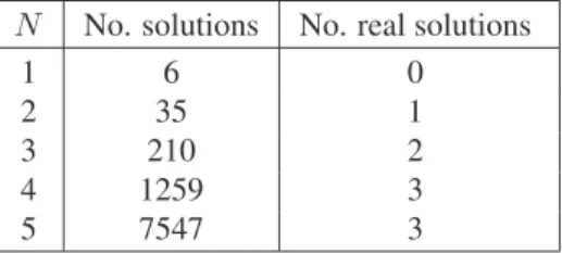
One can easily check thatF≺5Gon any intervalσ= [mσ−rσ, mσ+rσ]⊂R2. We can now apply the numerical homotopy method to solve (2), (3) withf(x, u, u′) =λexp(u) forλ=3, a value close to the turning pointλ⋆. We will use the exclusion test (24) with q=5 for the functions above until both components of the radii of the generated cells in Γlare less thanǫ=0.1. The results we obtained are shown in Tables 2 and 3.
N No. solutions No. real solutions
1 6 0
2 35 1
3 210 2
4 1259 3
5 7547 3
Table 2.mσ= (10,0)andrσ = (10,15).
N No. solutions No. real solutions
1 2 0
2 3 1
3 6 2
4 11 3
5 19 3
6 35 3
7 68 3
8 133 3
9 265 5
10 527 5
Table 3.mσ= (5,0)andrσ= (5,5).
Table 2 lists the number of solutions found using continuation intand the exclusion al- gorithm (24) with the starting cell given bymσ= (10,0)andrσ = (10,15). Table 3 lists the number of solutions found using continuation intand the exclusion algorithm (24) with the starting cell given bymσ= (5,0)andrσ= (5,5).
Remark 5.4.1. The exclusion algorithm process can be very costly and it is applied very often (every time we add a new interior point and for every solution on the previous grid).
For example, in Table 2, for adding one more point to the already existing four points implies using the exclusion algorithm 1259 times to solve equations of the form (21).
Also, to reach the goal ofkrσk ≤ ǫ, for anyσ ∈ Γl, we neededl =8 bisection levels each time we used the exclusion algorithm. Table 4 shows how the number of intervals σ∈Γlchanges aslincreases when using the exclusion algorithm to solve (21) as a fifth point is added to the already existing four interior points.
The bisection levell 0 1 2 3 4 5 6 7 8
Card(Γl) 1 4 16 64 247 870 1534 14 9 Table 4. Card(Γl) at each bisection levell.
The nine small cells at level 8 actually approximated six different solutions for (21).
This arises due to adjacency of surviving cells. Tables 2 and 3 illustrate the advisability of choosing an initial cell which is not too large, unless it is necessary.
Remark 5.4.2. For eachN =1, . . . ,5, all the solutions found in Table 3 have also been present in Table 2; this was expected since the cell chosen for the exclusion algorithm in Table 2 was bigger and included the one used in Table 3. Using interpolation of these real solutions (three for Table 2 forN = 5 and five for Table 3 forN =10) as initial guesses for Newton iterations, only two of them could be refined to more interior points.
For the other ones, the Newton process did not converge. The value ofuat the peaks for these two symmetric solutions atλ =3 with 1407 interior points are 0.6401 and 1.975 respectively.
6 Conclusions
While there is a dearth of theoretical results for existence, number and qualitative prop- erties of solutions for nonlinear PDE problems, we have seen that reliable information may be obtained through solving discretizations numerically by homotopy methods. First the system of equations is embedded into a complex setting. Next, when introducing a new mesh point, we use a method for finding all solutions to a single complex equation.
For polynomial equations we use the Matlab program which finds the eigenvalues of the corresponding companion matrix. For general nonlinearities, we have written a cellular exclusion program for finding the zeros of the real and imaginary parts. These steps fur- nish the starting points for tracing solution paths defined by a homotopy deformation of the mesh. We cannot throw away complex solutions found at the end of the homotopy, since as we have seen in Section 5.4 the real solutions sought may only arise after the discretization is sufficiently fine.
Techniques for findingallsolutions of systems have an important role to play. The methods presented in this paper are not meant to produce fast and accurate methods for solving PDE’s but rather the idea is to provide reliable information about the number of solutions as well as their qualitative properties. Furthermore, the approximations we obtain can be used as starting values to get more accurate solutions on finer meshes.
Appendix A Approximating the Laplacian In these appendices we use the notation,
• tis the homotopy parameter,
• lis the row in which the new mesh point is to be introduced,
• mis the number of rows of mesh points,
• nis the number of mesh points on each of the rowsl+1, . . . , m; hence, rows 1, . . . , l each hasn+1 points,
• N is the total number of mesh points; observe thatN =l(n+1) + (m−l)n, for t∈[0,1).
When we introduce a new point on thelth column()from the right, all the other points on thelthrow shift leftward as in the figure below. Remark that rows 1,2, . . . , l haven+1 points each, and rowsl+1, l+2, . . . , mhavenpoints each.
• ∆xold= b−an+1
• ∆xnew= b−an+2
• ∆yold= m+1d−c
• h(t) =t b−an+1
+ (1−t) b−an+2
• d(t) = (b−a)−(n+1)h(t) =· · ·= (1−t)b−an+2
For example, in Figure 10, the discretized solution~uof the system (10) will be written as
~u=
u1,1, u2,1, u3,1, u4,1, u1,2, u2,2, u3,2, u4,2, . . . , u1,5, u2,5, u3,5
T 18×1.
Figure 10. Introducing a new point()on thelthrow.
Remark. Notice the way we order the unknownsui,j inside of the vector~u. When a new point will be introduced on a column (from above for example) instead of a row, the unknownsui,jinside of the vector~uwill be ordered differently (to keep the sparsity
structure of the stiffness matrixA). In this case, the vector~uwill have the form
~u=
u1,1, u1,2, u1,3, u1,4, u1,5, u2,1, u2,2, . . .T
.
Appendix A.1 All rows exceptl−1, l, andl+1. We can easily approximate the Laplacian at all the points which are not on the rowsl−1, l, andl+1 by
• Formula for(uxx)j,k
(uxx)j,k≈ uj−1,k−2uj,k+uj+1,k
∆x2 ,
forj=1, . . . , n(orn+1),k=1, . . . , m,k6=l, where
∆x=
(∆xnew if 1≤k≤l−1
∆xold ifl+1≤k≤m.
• Formula for(uyy)j,k
(uyy)j,k≈uj,k−1−2uj,k+uj,k+1
∆y2 ,
forj=1, . . . , n(orn+1),k=1, . . . , m,k /∈ {l−1, l, l+1}, where∆y= ∆yold.
Figure 11. Introducing a new point()on thelthrow. Approximating the Laplacian at the points on the(l−1)throw.
Appendix A.2 Rowl−1. On the(l−1)throw we have the following.
• Formula for(uxx)j,l−1
(uxx)j,l−1 ≈uj−1,l−1−2uj,l−1+uj+1,l−1
∆x2 ,
forj=1, . . . , N+1, where∆x= ∆xnew.
• Formula for(uyy)j,l−1
(uyy)j,l−1≈ uj,l−2−2uj,l−1+ ˜uj
∆y2 ,
forj=1, . . . , n+1, where∆y= ∆yold;u˜j:=uj−1,l+rj·(uj,l−uj+1,l), where rj= j∆xnew−(j−1)h(t)
h(t) .
Hence,
(uyy)j,l−1≈ (1−rj)uj−1,l+uj,l−2−2uj,l−1+rjuj,l
∆yold2 ,
forj=1, . . . , n+1.
Appendix A.3 Rows l and l + 1. In a similar manner, one needs to take care of approximating the Laplacian at the interior points on thelthand on the(l+1)throws.
Appendix B The components of the homotopyHn
Axxis a block diagonal matrix of the form1
Axx= diag(T1, . . . , T1, T2, T3, . . . , T3)
whereT1,T2,T3are tridiagonal square matrices of sizesN+1,N+1, andN, respectively T1 = ∆x12
newS,T3 = ∆x12 old
S,T2 = h(t)1 2S, whereSis a tridiagonal matrix having−2 on the main diagonal and 1 on the upper and lower diagonals.
~bxxis ablockvector of the form
~bxx= ~b1(y1), . . . ,~b1(yl−1),~b2(yl),~b3(yl+1), . . . ,~b3(ym)T
where~b1,~b2,~b3are sparse vectors of sizes 1×(n+1), 1×(n+1), and 1×n, respectively:
~b1(yj) = 1
∆x2new(ua(yj),0, . . . ,0, ub(yj)),
~b2(yj) = 1
h(t)2(ua(yj),0, . . . ,0, ub(yj)),
~b3(yj) = 1
∆x2old(ua(yj),0, . . . ,0, ub(yj)).
1In the structure ofAxx, there arel−1 blocksT1andm−lblocksT3.
![Table 1. The number of solutions for ∆u = − (1 + u 2 ) on Ω = [0, 1] × [0, 1] with zero Dirichlet boundary conditions.](https://thumb-eu.123doks.com/thumbv2/1library_info/5606987.1691320/12.892.213.722.360.906/table-number-solutions-ω-zero-dirichlet-boundary-conditions.webp)