0 1998 IUPAC
INTERNATIONAL UNION OF PURE AND APPLIED CHEMISTRY
PHYSICAL CHEMISTRY DIVISION COMMISSION ON THERMODYNAMICS
NOMENCLATURE FOR PHASE DIAGRAMS WITH PARTICULAR REFERENCE
TO VAPOUR-LIQUID AND LIQUID-LIQUID EQUILIBRIA
(Technical Report)
Prepared for publication by
ANDREAS BOLZ,~ ULRICH K. DEITERS,' COR J. PETERS^ AND THEO w. DE LOOS~
Institute for Physical Chemistry, University at Cologne, F.R. Germany
Laboratory of Applied Thermodynamics and Phase Equilibria, Delft University of Technology, the Netherlands
Membership of the Commission on Thermodynamics (1.2):
Titular Members: Prof. R. D. Weir (Chairman, 1994-1999); Dr J. H. Dymond (Secretary, 1990-1999); Prof.
T. W. de Loos (1994-1999); Prof. U. K. Deiters (1998-1999); Prof. J. P. E. Grolier (1996-1999); Prof.
T. M. Letcher (1998-1999).
Associate Members: Prof. J. C. Ahluwalia (1994-1999); Prof. J. A. R. Cheda (1998-1999); Prof. V. A. Durov (1996-1999); Prof. A. R. H. Goodwin (1996-1999); Dr K. P. Murphy (1996-1999); Prof. M. A. V. Ribeiro da Silva (1994-1999); Prof. A. Schiraldi (1998-1999); Prof. M. Sorai (1998-1999); Prof. S. Stolen (1998-1999);
Prof. E. Vogel(1994-1999); Prof. Mary Anne White (1998-1999).
National Representatives: Prof. C. Airoldi (Brazil, 1992-1999); Prof. H. K. Yan (Chinese Chemical Society, 1996- 1999); Prof. T. Boublik (Czech Republic, 1996-1999); Prof. FranGoise Rouquerol (France, 1988-1999); Prof.
H. Pak (Korea, 1996-1999); Prof. G. Kaptay (Hungary, 1998-1999); Dr J. L. Laynez (Spain, 1994-1999); Prof.
I. Wadso (Sweden, 1994-1999).
Subcommittee on Thermodynamic Data
Members: Prof. U. K. Deiters (Chairman); Dr M. Trusler (Secretary); Prof. Y. Arai; Prof. J. Barthel; Mrs. K. M. de Reuck; Prof. A. Heintz; Dr V. Majer; Dr K. Marsh; Dr Jadwiga Sipowska.
Subcommittee on Transport Properties
Members: Prof. W. A. Wakeham (Chairman); Prof. M. J. Assael (Secretary); Prof. A. Leipertz; Prof.
A. Nagashima; Prof. C. A. Nieto de Castro; Prof. H. A. Oye; Prof. J. V. Sengers.
Republication or reproduction of this report or its storage andor dissemination by electronic means is permitted without the need for formal IUPAC permission on condition that an acknowledgement, with full reference to the source along with use of the copyright symbol 0, the name IUPAC and the year of publication are prominently visible. Publication of a translation into another language is subject to the additional condition of prior approval from the relevant IUPAC National Adhering Organization.
2233
2234 COMMISSION ON THERMODYNAMICS
Nomenclature for phase diagrams with particular reference to vapour-liquid and liquid-liquid
equ i I i bria (Technical Report)
Abstract: The phase diagrams of binary fluid mixtures are classified with regard to the topology of their critical curves and three-phase curves. A new nomenclature for the phase diagram classes is proposed, which can be applied to the previously known as well as to recently discovered phase diagram classes. The class names of the new nomenclature are systematic and descriptive; the (P,T) projection of a binary fluid phase diagram can always be constructed qualitatively from the class name.
INTRODUCTION
Phase equilibria in binary systems are usually depicted graphically in pressure, temperature, composition (P,T,x) space, in (P,T) and (T,x) projections or in isothermal (PJ) sections, isobaric ( T J ) sections and in constant composition (P,T) sections, so called isopleths. In these diagrams the different types of phase equilibria are represented by areas, curves or points. Some of these equilibrium states are characterized by special values of thermodynamic variables and will be referred to as special states. In the scope of this work a special state or point is defined as a state or point where
1. Either a phase is added or disappears.
2. Where the composition of two phases become identical.
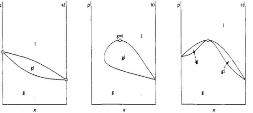
The composition of two phases can become identical in three different ways (Rowlinson & Swinton, 1982). The curves representing the composition of two coexisting phases can intersect at x = 0 or x = 1.
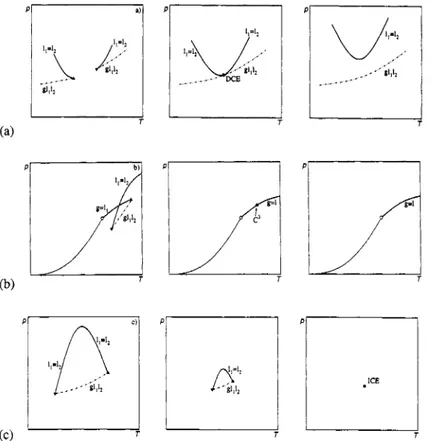
This is shown in Fig. la, which shows a vapour-liquid equilibrium gl where the curve that represents the composition of the liquid phase 1 intersects the curve for the vapour phase g in the boiling points of both pure components. Also these curves can merge in a horizontal tangent point (dT/dx), = 0 or ( d P / d ~ ) ~ = 0.
This type of special point is a critical point, where not only the composition but all thermodynamic properties of the two phases become identical. A diagram with a critical point is shown in Fig. lb. The third possibility is that the two curves have a common horizontal tangent. In this case only the compositions of the two phases are equal, but not the other thermodynamic properties. An example is an azeotropic point (Fig. lc).
p~
X X X
Fig. 1. Three cases where the compositions of the two phases of a two-phase equilibrium are equal. (a) Pure component boiling points. (b) Critical point g = 1. (c) Azeotropic point (gl)u.
In literature and text books many confusing terms are used to describe special states of binary fluid mixtures. People working in the field of fluid phase equilibria feel a need for one specific term for these
0 1998 IUPAC, Pure and Applied Chemistry70,2233-2257
special states. The only existing systematic nomenclature is that of Griffiths (1975), which is not detailed enough and which is hardly ever used.
Closely related to this problem is the nomenclature for fluid phase diagram classes. In the last decades many new types have been discovered from mathematical analysis of computational models (Furman et al., 1977; Mazur et al., 1984; Mazur et al., 1985; Boshkov & Mazur, 1986; Boshkov, 1987; van Pelt et al., 1991), which can not be classified in a logical way by extension of the classification scheme of van Konynenburg & Scott (1980), which is discussed extensively in Rowlinson & Swinton (1982). In this case there is the need for a general classification scheme, which can be used to classify the known types of fluid phase behaviour and which is flexible enough to include today unknown types of fluid phase behaviour.
In this paper a new nomenclature for phase diagram classes of binary fluid mixtures is presented and recommendations for nomenclature for special states of these mixtures are given. Also recommendations for the graphical representation of these special states are included.
NOMENCLATURE FOR SPECIAL STATES OF FLUID MIXTURES
According to the phase rule, which reads for a non reacting system with N components F = N - l7+ 2 - @
the phase behaviour of a binary system can be represented in a three-dimensional pressure, temperature, composition (P,T,x) space. l 7 i s the number of phases in equilibrium, F is the number of degrees of freedom and @ is the number of extra relations that hold in a special state. Usually for the composition variable the mole fraction x is used. Different types of phase equilibria in binary systems and their representations in (P, T,x) space are given in Table 1. In the example of the critical point in Fig.
Ib l7= 1 and I$ = 2 and in the example of the azeotropic point in Fig. Ic l7= 2 and @ = 1. For a binary system the maximum number of phases in equilibrium is four, the minimum number of degrees of freedom is zero.
Since it is tedious to draw three-dimensional diagrams in perspective, it is common practice to use two- dimensional sections and projections of the (P,T,x) space to represent the phase behaviour of a binary system. Sections at constant temperature are called (PJ) sections, at constant pressure
(Zx)
sections and at constant composition (P, T ) sections or isopleths. Among the projections, the projection on the (P,T) plane, the (P,T) projection, is the most common. Of course, the sections and projections do not contain the complete information of the (P,T,x) space, e.g., in projections only information on nonvariant ( F = 0) and monovariant ( F = 1) equilibria can be found.
Table 1. Phase equilibria in binary systems and their representation in (P,T,x) space, with x = x2, Z7is the number of coexisting phases and F the number of degrees of freedom according to the phase rule.
Representation in (P, T,x) Examples
I7= 1 F = 3 region s17 s2.1, g, 11, 12, s
I7= 2 F = 2 two surfaces: xa(P, Tj; xP(P, Tj gl, Sll, 1112 critical curve I7= 1 F = 1 x'[P(T)] g = 1, 11 = 12 Z7= 4 F = 0 four points at one P and T s1gls2, g1112s critical endpoint I7= 2
I 7 = 3 F = 1 three curves: xr[P(T)]; xP[P(T)l; x/[P(T)l slgl, s11s2, llg12 azeotropic curve I7= 2 F = 1 x"[P(T)]
F = 0 two points at one P and T g(l1 = 12L (g = 11Y2, s(g = 1)
critical azeotrope Z7= 1 F = 0 one point
The variables P and T and the variable x are of a different nature (Griffiths & Wheeler, 1970). P and T are "field" variables, variables that have the same value for all coexisting phases and the mole fraction x is a "density" variable, a variable which has in general a different value from phase to phase. Phase diagrams can also be represented in graphs using only fields as variables. This is not common practice,
0 1998 IUPAC, Pure and Applied Chernistry70,2233-2257
2236 COMMISSION ON THERMODYNAMICS
but it has the advantage that the phase diagram only shows the intrinsic features of the phase behaviour and not the "accidental" consequences of the choice of the coordinates (Furman et al., 1977). For instance, for a three-phase equilibrium in a binary system we have F = 1. Such an equilibrium is represented by three curves in (P,T,x) space, because the composition of the three phases is different at one P and T, but this equilibrium is represented by one curve in a three-dimensional diagram using P, T and the chemical potential of one of the components as variables, which are all "fields".
The term global phase diagram has been introduced by Furman et al. (1977). This type of phase diagram is generated by a theory or a model, using the molecular parameters of the model as additional field variables. From this multi-dimensional global phase diagram also two-dimensional projections or sections can be constructed. An example of such a two-dimensional global phase diagram is the i;
A
masterchart of van Konynenburg & Scott (1980) for constant
5.
These authors used the van der Waals equation of state with<= (~22~7222 - ~llh11~)/(a22h222 + allhl12)
A
= ( a l l h 2 - 2a1241b22 + a2249222)/(a22h222 + a d h 2 ) { = (b22 - biJ(b22 + bii)as additional field variables. a l l and bll are the pure component van der Waals constants. A region in this master chart represents one of the classes of fluid phase diagrams, which are discussed in the section A new nomenclature for phase diagram classes of binary fluid mixtures.
In the following we propose a nomenclature for special states in phase diagrams for binary fluid systems, which is more informative than the notation suggested by Griffiths (1975). These states will be arranged in levels. Level n means that the number of degrees of freedom according to the phase rule for states in this level is F = (3 - n). A binary system with components A and B can be denoted with [A
+
B], [xAA+
xBB] or [(l - x)A+
xB], where x is the mole fraction of component B. In this paper we will use the last notation. The states of aggregation will be denoted with g (gas or vapour), 1 (liquid) or s (solid), according to the IUPAC recommendations (Mills et al., 1993). The distinction between gas and liquid is to some extent arbitrary. A fluid phase (i.e. gas or liquid) can be denoted with f. In binary systems more than one solid phase and more than one liquid phase can coexist. In general these phases have a different composition. A right subscript 1, 2 can be used to distinguish between these phases. In the notation for multiphase equilibria it is advised to list the phases in the order of increasing x.Example slgll is the recommended notation for a three-phase equilibrium with phases sl, g, and l1 For all states discussed in level 4 and higher the number of degrees of freedom F is negative and hence it is very unlikely that these states can be realized experimentally in a binary system. These special states are mainly of interest to theory and especially help us to understand the transitions between the various types of phase diagrams.
(X(Sl)< x(g> < X(l1)).
Level 0: volume in (P,T,x) space
For F = 3,17= 1 and we are dealing with a homogeneous phase. Griffiths denoted this state with A. We advise to use s, 1 or g.
Level 1: area in (P,T), (P,x) or (T,x) section
For F = 2, 17= 2 and we are dealing with two-phase equilibria. All these states were denoted AA or A2 by Griffiths. Again we recommend to use a more informative notation, like gs, gl, 1112, or gll equilibria.
Level 2: curve in (P,n projection
In this case F = 1 and we are dealing either with a critical curve, with the coexistence of three phases, or with the coexistence of two phases with the same composition.
0 1998 IUPAC, Pure and Applied Chemistry 70,2233-2257
Coalescence of two phases
In our nomenclature a critical curve is denoted with C, or more specific, depending on the nature of the critical curve, with g = 1, l1 = 12, l1 = g, etc. An upper or lower critical point is indicated with UC or LC, respectively. For instance, a lower critical (solution) temperature can be denoted with LC, , where the subscript P means "at constant pressure", and an upper critical (solution) pressure with UCT. The notation UC and LC defaults to UCp and LC,, respectively. In ( P J ) , ( T J ) and (P,T) sections the critical state is represented by a point, for which the same nomenclature can be used. The critical state was denoted by Griffiths with B.
Coexistence of three phases
The recommended notation for a three-phase curve is g1112, llg12, slgl, s11s2, etc., depending on the nature of the three-phase curve. The notation of Griffiths for a three-phase equilibrium is AAA or A3.
Coexistence of two phases with the same composition
If, in case of a two-phase equilibrium, the compositions of the two phases are equal as in the case of an azeotrope, then according to the phase rule F = 1. We propose to use the notation (gl), for the azeotropic curve in (P,T,x) space, and in (P,T) or ( T J ) projection and also for the azeotropic point in (TJ), ( P J ) , or (P,T) sections. Further distinction can be made between a maximum pressure and a minimum pressure azeotrope. The notation used by Griffiths (A*=) is too general, because similar points can be found for other phase equilibria, e.g. of sl two-phase equilibria.
Temperature or pressure maximum of an isopleth
Often the temperature maximum of the gl equilibrium in a (P,T) section is called maxcondentherm or cricondentherm and the pressure maximum maxcondenbar or cricondenbar (Rowlinson & Swinton,
1982). These points do not represent special states according to the definition.
Level 3: point in (P,q projection, area in two-dimensional global phase diagram Extrema of the critical curve in (P, T ) projection
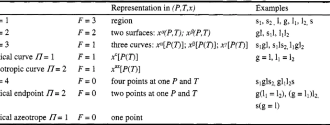
A pressure maximum of the critical curve in the (P,T) projection is not a special point of the critical curve. However, it brings about a special point in the (T,x) section at the pressure of the pressure maximum (see Fig. 2). In Fig. 2a on pressure increase the two-phase region ap disappears, since we are dealing with upper critical pressures. In Fig. 2b two separate two-phase regions ap join on pressure increase. Schneider (1966) used the term hypercritical point of the first kind for the pressure maximum of the critical curve for the case of Fig. 2a and hypercritical point of the second kind for the pressure maximum of the critical curve for the case of Fig. 2b. This latter point was called homogeneous double ylait point by van der Waals & Kohnstamm (1927). Since the term hypercritical should be reserved for another phenomenon and we are not dealing with a double point of the critical curve, we propose simply to call a pressure maximum of the critical curve a maximum pressure critical point. To differentiate between the case of Fig. 2a and that of Fig. 2b, the pressure maximum of the critical curve in Fig. 2a can be called an elliptic maximum pressure critical point and that in Fig. 2b a hyperbolic maximum pressure critical point.
The critical curve can also show pressure minima and temperature maxima and minima in a (P,T) projection. Following the proposed terminology for a pressure maximum, these points can be denoted with minimum pressure critical point, maximum temperature critical point and minimum temperature critical point, if necessary with the addition elliptic or hyperbolic.
Critical phase coexisting with another (noncritical) phase: critical endpoint
A three-phase curve in a binary system involving two or three fluid phases can be terminated in a (P,T) projection by a so-called critical endpoint in case of coalescence of two fluid phases ( F = 1) in the presence of the third phase. The notation of Griffiths for this kind of special point is BA. The critical
Q 1998 IUPAC, Pure and Applied Chemistry70,2233-2257
2238 COMMISSION ON THERMODYNAMICS
P
endpoint can be the lower or the upper temperature limit of a three-phase curve. These endpoints are conventionally called lower critical endpoints or, respectively, upper critical endpoints". It is also possible that a critical endpoint is the low pressure or the high pressure limit of a three-phase curve.
a) one phase
p, ---
- n B
I I
T
(a) X X
1
P = h U 1
X
X X X
Fig. 2. A critical curve a = p with a pressure maximum. (a) Two critical points coincide such that the two-phase region disappears: an elliptic maximum pressure critical point. (b) Two two-phase regions join at the pressure maximum of the critical curve: an hyperbolic maximum pressure critical point. 0 : critical point.
*Sometimes the distinction between upper and lower critical endpoint is not clear. In these cases it is better not to make a distinction at all.
Q 1998 IUPAC, Pure and Applied Chemistry70,2233-2257
To be in line with the proposed notation for critical points we propose to denote a critical endpoint with CE. A critical endpoint which is the low-temperature limit of a three phase curve can be denoted with LCE(T) and a critical endpoint which is the high-temperature limit of a three-phase curve can be denoted with UCE(7'). These critical endpoints are conventionally denoted with LCEP and UCEP, which has the disadvantage that no distinction can be made with critical endpoints that limit a three-phase curve towards low or high pressure. For these critical endpoints we propose to use LCE(P), respectively UCE(P). The notation LCE and UCE is by default the notation for a critical endpoint which limit a three-phase curve towards low or high temperature, respectively. For some types of phase diagrams the UCE(T) is denoted with K-point and the LCE(7') with L-point. This notation, which is mainly used by American authors, is non-systematic and we advise not to use it.
Examples of critical endpoints are g(ll = 12) and (g = l)sz equilibria.
Azeotrope coexisting with another (noncritical) phase
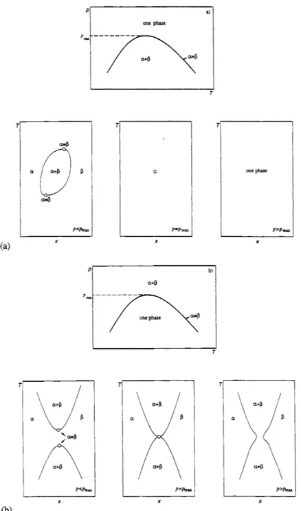
In the P-T projection an azeotropic curve can end on a three-phase curve. In this point, which is called azeotropic endpoint, the three-phase curve and the azeotropic curve are tangent. This type of point was indicated with A2,A by Griffiths. We propose a more informative notation, which includes the nature of the phases involved and which is in line with the proposed notation for two- and three-phase equilibria, e.g., (g11),12 (Fig. 3a) or s(gl),, (Fig. 3b).
Fig. 3. Azeotropic endpoints. (a) (gll)&. (b) s(gl),. (c) Limiting azeotrope -
-
- - - - - : three-phase curves;---- : azeotropic curves; : vapour pressure curve.
Coalescence of two azeotropic phases
Another possible limit of an azeotropic curve is a critical azeotropic point or critical azeotrope. This point is a point where the azeotropic curve is tangent to a g = 1 curve. For this reason we propose to denote this point with (g = l),. Griffiths' notation for a critical azeotrope is Baz.
Azeotrope at x = 0 or x = 1
Furthermore an azeotropic curve can end in a tangent point on a pure-component vapour-pressure curve (Fig. 3c). This case is called a limiting azeotrope or an azeotropic boundary. If necessary this point can be denoted with (gl)az(x = 0) or (gI),& = 1).
Intersection (only in (P, T ) projection) of pure-component vapour pressure curves
This point of intersection, which is sometimes called Bancroft-point (van Konynenburg, 1968), is only a point of intersection in the (P,T) projection and we do not recommend the use of a special notation.
Critical point on the boundary of local stability
This point is a point on the critical curve where a4G/ax4 = 0 and it separates the stable or metastable part of the critical curve (a4G/ax4 > 0) from the unstable part of the critical curve (a4G/ax4 c 0). This point, which was named heterogeneous double plait point by van der Waals & Kohnstamm (1927), is a cusp-like double point of the critical curve in the ( P , n projection; hence, we propose to name this type
C31998 IUPAC, Pure and Applied Chemistry70,2233-2257
2240 COMMISSION ON THERMODYNAMICS
of point a critical cusp and denote it with CC. (See Fig. 4). Critical cusps are usually not stable, and hence cannot be observed experimentally.
Coexistence of four phases
The (P,r) projection of the four points which represent the composition of a four-phase equilibrium in (P,T,x) space is one point. This point is called quadruple point and in line with the conventional notation we propose to denote this point with Q. Griffiths' notation for this equilibrium is &. Examples are glllzls, slglsz, gll12s2 , and s11112s2 equilibria.
Fig. 4. A critical cusp (CC). - : stable part of the critical curve;
...
: metastable part of the critical curve; ---: unstable part of the critical curve; - - - -: three-phase curve; A: upper critical endpoint.Level 4: line in a two-dimensional global phase diagram Osculation point of a critical curve and a three-phase curve
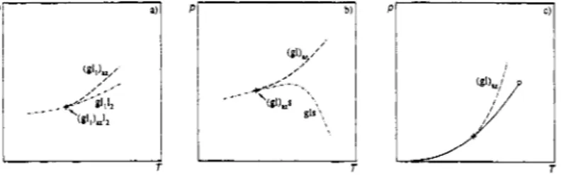
The osculation point of a critical curve and a three-phase curve in a (P,T) projection is called a double critical endpoint (van Konynenburg, 1968). In this point two critical endpoints of the same nature and on different three-phase curves coincide, such that the three-phase curves are joined (see Fig. 5a). In a binary phase diagram such a situation is very unlikely to be observed experimentally ( F = -1). We propose to denote this equilibrium with DCE. Examples are the coincidence of two g(ll = 12) or two (g = l,)lz critical endpoints.
Coincidence point of two critical endpoints of a different nature on the same three-phase curve, such that the three-phase curve collapses
This special point is a point of coalescence of three phases. It can also not be realized in a binary system and is called (unsymmetrical) tricritical point. The notation of Griffiths for such a point is C. Because we propose to denote an ordinary critical point with C, we propose to use the notation C" for a higher order critical point. n is the number of phases that become identical. So our proposed notation for a tricritical point is C3. An example is the coincidence of an LCE g(ll = 12) with an UCE (g = 11)12 on the same three-phase curve g1112 in such a way that the length of the three-phase curve in the (P,r) projection becomes zero (see Fig. 5b).
Coincidence point of two critical endpoints of the same nature on the same three-phase curve, such that the three-phase curve collapses
For this special point we propose the name isolated critical endpoint and the notation ICE. Again this special point can not be realized in a binary system. An example is the coincidence of a LCE g(ll = lZ) with an UCE g(ll = 12) on the same three-phase curve gll12 in such a way that the length of the three-phase curve in the (P,r) projection becomes zero (see Fig. 5c).
Critical azeotrope coexisting with another (noncritical) phase
Griffiths' notation for this critical azeotropic endpoint is B,A. We propose the notation CE,,.
0 1998 IUPAC, Pure and Applied Chernistry70,2233-2257
Critical phase in the presence of two noncritical phases
We propose to name this point bicritical three phase point and to denote it with BT. Griffiths' notation for this point is BA2. An example is a (g = 11)12s2 equilibrium.
1,=11
1,=1*
p
. . c'' &I*
_ -
..II
T
Fig. 5. Two critical endpoints coincide. (a) A double critical endpoint (DCE). (b) A tricritical point (C ). (c) An isolated critical endpoint (ICE).
-
: stable part of the critical curve; - - - - - - -: three-phase curve;critical endpoints.
: pure component vapour pressure curve; 0: pure component critical point; A, V: upper and lower
Collision of two critical curves
When two separated parts of the critical curve meet and exchange branches we are dealing with a double point of the critical curve. Two cases can be distinguished. In the first case two critical cusps coincide.
See Fig 6a. Often this point is referred to as an unstable mathematical double point. In line with the above we propose to name this type of point double critical cusp and to denote it with DCC.
P
Fig. 6. Collision of two critical curves. (a) Coincidence of two critici x s p s in a double critical cusp (DCC). (b) Coincidence of two stable branches of a critical curve in a hypercritical point (HC). :- stable part of the
- - - : three-phase curve; A, V: upper and lower critical endpoints.
critical curve;
. ... ... ... .
metastable part of the critical curve; ---: unstable part of the critical curve;0 1998 IUPAC, Pure and Applied Chemistry70,2233-2257
2242 COMMISSION ON THERMODYNAMICS
In the second case two stable branches of the critical curve meet (see Fig. 6b). This type of double point has been referred to as stable mathematical double point. For this point we propose the name hypercritical point and the notation HC.
Level 5: point in two-dimensional global phase diagram Tricritical point coexisting with another (noncritical) phase
We propose to name this point tricritical endpoint or tricritical quadruple point with the notation C3E or C3Q. Griffiths' notation for this type of point is CA. An example is a (g = l1 = 12)13 equilibrium.
Coincidence of a tricritical point and double critical endpoint
After Meijer et al. (1988) we propose to name this type of point van b a r point with the notation VL.
Jackson (1991) named this type of point tricritical endpoint, but this name is not in line with the nomenclature of ordinary critical points and critical endpoints. Also this type of point has been referred to as symmetrical tricritical point.
Level 6: point in three-dimensional global phase diagram Coalescence of four phases
In line with the name and notation for a tricritical point we propose the name tetracritical point and notation C4 for a fourth order critical point where four fluid phases become identical. Griffiths' notation for a fourth order critical point is D.
RECOMMENDATIONS FOR THE GRAPHICAL REPRESENTATION OF BINARY PHASE DIAGRAMS
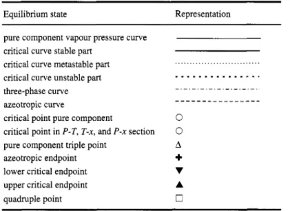
Although less important than an unique nomenclature for special states in phase diagrams it can also be useful to use a unique graphical representation for the different types of equilibria. In Table 2 a proposal is given for the representation of nonvariant and monovariant states in (P, r ) projections.
Table 2. Graphical representation of nonvariant and monovariant states
Equilibrium state Representation
pure component vapour pressure curve critical curve stable part
critical curve metastable part critical curve unstable part three-phase curve azeotropic curve
critical point pure component
critical point in P-T, T-x, and P-x section pure component triple point
azeotropic endpoint lower critical endpoint upper critical endpoint quadruple point
0 0 A
+
v
A 0
0 1998 IUPAC, Pure and Applied Chernistry70,2233-2257
A new nomenclature for phase diagram classes of binary fluid mixtures
In his 1968 dissertation on global phase behaviour of binary fluid mixtures, P. van Konynenburg found five different classes of phase diagrams, to which he gave the names I to V. Today, more than 16 basic classes are known. The additional phase diagram classes are usually referred to by a roman number in connection with a modifier (*,
**,
and/or subscript 4, subscript b or superscript h). However, the meaning of the modifier symbol is not always the same. This nomenclature, the product of a number of different research groups , is very confusing. Therefore, we want to present a new system of names which is able to describe all known and yet unknown phase diagrams in a rational way.Rational nomenclature
The nomenclature described here regards primarily the topology and connectivity of critical curves. The vapour-pressure curves of the pure components are always present and need not to be designated explicitly. The number and extent of three-phase curves, if present, can be deduced from the location of the critical curves and their endpoints, hence only the latter curves and points need to be designated. The construction of a rational phase diagram is done in four steps:.
1. The critical point of a pure component is always the starting point of a critical curve or a sequence of critical curves connected by three-phase lines. We begin by describing the behaviour of the critical curve starting at the critical point of the component with the higher critical temperature. All critical curve segments in the sequence originating from this point are counted; next the "target" of this sequence is indicated with a superscript. Possible targets are:
C
P
2
Q
for sequences going upwards to a compact fluid state at very high pressure. Many theories of fluid mixtures use the concept of limiting critical states at infinite pressure,
for sequences ending at the critical point of the other pure component,
for sequences terminating at a critical endpoint, from which a three-phase curve emerges which terminates at absolute zero of temperature,
for curves going to an endpoint from which a three-phase curve runs to a quadruple point (4 fluid states in equilibrium). Usually another three-phase curve runs from here to absolute zero temperature. If no different topology of the quadruple point is specified by other critical curve symbols, this three-phase curve and its target are implied by the Q symbol and must not be mentioned in the class name.
If this part of the diagram is not known, this can be indicated by Xfarger, or, if also the target is unknown,
x'.
The behaviour of the critical curve sequence starting at the critical point of the lower boiling
component is described. However, if the target of the critical curve sequence described in step 1 is P (the critical point of the other pure component), this description is not necessary.
Critical curves which were not counted in steps 1 and 2 are classified as follows:
1 2.
3.
curves coming from high pressure (C state) and going to a critical endpoint; in practice, of course, 1-type critical curves end on crystallization surfaces,
curves with two critical endpoints,
curves coming from high pressure and going through a pressure minimum back to high pressure, which have no endpoints (if solidification is disregarded),
II
u
o closed loops.
These symbols have been chosen to mimic the shape of the critical curves.
With these symbols, the remaining critical curves are now listed in the order of their appearance from high to low temperature. Except in clear cases, the target or targets (names of the connected curves) must be written as superscripts. Parentheses can be used to group critical curves forming a sequence, i.e., joined by three-phase curves. If this is still ambiguous, it is necessary to label each critical curve with a Greek character subscript and use this symbol as target indication.
0 1998 IUPAC, Pure and Applied Chemistry70,2233-2257
2244 COMMISSION ON THERMODYNAMICS
4. It may be desirable to follow these symbols with detailed information. The following abbreviations should be used:
H for heteroazeotropic behaviour, A for azeoptropy,
Q for quadruple point,
M for pressure maxima; the number of maxima may be indicated by a superscript, W for pressure minima: the number of minima may be indicated by a superscript.
This information usually refers to a specific sequence, so it must be written directly behind this sequence symbol. To connect it to a particular line of a sequence starting at a pure component, it is possible to write the whole sequence in parentheses.
Sometimes it may be important to give more information. This could be given after a decimal point.
Also, it may be desirable to include information about solid phases. This could follow after a slash (/); a nomenclature system has yet to be designed.
5.
EXAMPLES
Several examples for the construction of the rational phase diagram names are given in this section.
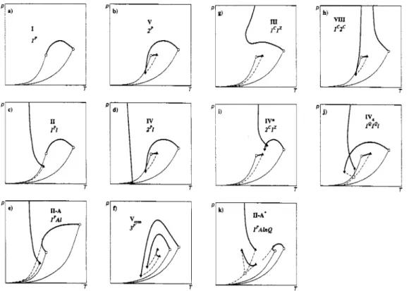
Furthermore, a translation table of the van Konynenburg class names as well as some of the new names is given in Table 3, and schematic (P,T) phase diagrams of some of the most important phase diagram classes are shown in Fig. 7.
I b) V
9
P b l
I
'I'
T P 0
i & i
II,,T
p s i
I
T
Fig. 7. Phase diagram classes of binary fluid mixtures. - : vapour-pressure curves; *-
.
criticalcurves; - - - - - - -: three-phase curves; - - - -: azeotropic curves; 0: pure component critical points; 0:
quadruple point; A, V: upper and lower critical endpoints, +: azeotropic endpoints.
Q 1998 IUPAC, Pure and Applied Chemisrry70,2233-2257
Fig. 7. Continued.
In the phase diagram class I (van Konynenburg-Scott nomenclature) only one critical line exists, which connects the critical points of the pure components. The new class name is therefore 1' (see Fig.
7a). For class I1 a liquid-liquid critical line is added: 1'1 (Fig. 7c).
In class IV, a critical curve runs from the critical point of the less volatile component to a lower critical endpoint. From here a three-phase curve runs to an upper critical endpoint, and from here a critical curve to the other pure component critical point. Hence the critical curve sequence has two critical segments. In addition, there is a liquid-liquid critical curve. The new class name is therefore 2'1.
A lengthier, but admissible alternative name is (nn)'Z (here the pure component critical points are treated as endpoints). This latter expression is useful, if additional characteristics of a critical curve need to be specified. For instance, if the critical curve originating at the critical point of the less volatile component passes through a maximum, this could be specified by (nMn)'Z. The "transition" phase diagram between all 1' and 2' phase diagrams contains a tricritical point (see Fig. 5b).
The shield region class 11-A* (Fig. 7k) can be translated into 1'AnlQ or l'AnQQZQ. The latter name is longer, but does not contain more information: A quadruple point is the intersection point of four three-phase lines, one of which is usually connected to absolute zero. The three remaining three-phase curves originate at the endpoints of the n and 1 critical lines. Since no other combination is possible, it is not necessary to give the target three times, and the shorter name l'AnlQ is sufficient.
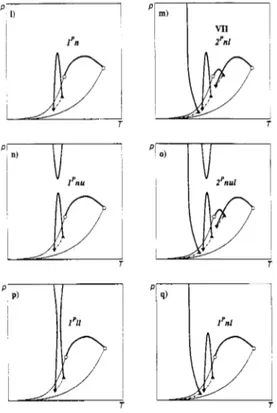
For some mixtures containing strongly polar compounds closed immiscibility domains have been observed (van Konynenburg-Scott class VI). This is caused by a n critical curve segment; the new class name is therefore 1'n (see Fig. 71). It has been suggested that in this class an additional low-temperature liquid-liquid critical curve might appear (Boshkov, 1987); this would change the name to 1'nl (see Fig.
7q). If a high-pressure immiscibility is found, the class name becomes l'nu (see Fig. 7n). If high- and low-pressure immiscibility domains overlap (compare Figs. 7n & 7p), a new diagram type is created which has no name in the old nomenclature system. The new name is 1% or, more precisely, l'(11). The parentheses indicate that the two 1 critical curves form a sequence, i.e., that they are joined by a three-phase curve. But since there are no other ways of placing the two 1 critical curves without leaving
0 1998 IUPAC, Pure and Applied Chemistry 70,2233-2257
2246 COMMISSION ON THERMODYNAMICS
one three-phase curve open-ended, the parentheses are not strictly necessary. The "transition" phase diagram between nu and (11) contains a hypercritical point.
Table 3. Comparison of phase diagram class names according to the van Konynenburg-Scott system and the rational nomenclature.
Old nomenclature New nomenclature Figure I
I1 11-A*
I11 111-A*
111-A"*
IV IV*
1v;
V W Iv4 V VI
vlb
VII VIP VIII
1' 1' 1 lPAlnQ l'AlnQ lCIQAn l C I Q nA 2' 1 2c1z l Q l Q l 2p 3' l'nl l'nul 22'nl 2'nul 1 c2c 2'lnQ
7a 7c 7k 7g
7d 7i 7J 7b 7f 71 7m 7h
DISCUSSION
For all realistic phase diagram classes which are known until now, the new nomenclature leads to reasonably short, but nevertheless descriptive names.
The nomenclature is based on observable curves only. This is an advantage for its application to experimentally determined phase diagrams. In some lattice gas theories, the high pressure target ( C ) is shown to bear some analogy to a pure component critical point (Furman et al., 1977; Furman & Griffiths, 1978). This fact might be used to devise a more "symmetric" nomenclature of phase diagrams for such theories. More realistic models, however, may have more than one high-pressure target (Deiters &
Kraska, 1992). Hence it would be impossible to classify a real mixture correctly by comparison with lattice models.
The old nomenclature has the disadvantage that the addition of a new feature to a phase diagram leads to a completely new class name. E.g., if a mixture has been classified as type I because of VLE measurements, and if later on a low-temperature liquid-liquid phase splitting is discovered, the class name must be changed to "II", and the assignment "I" must be considered wrong. With the new nomenclature system, the class name merely changes from 1' to 1'1. Thus the correct knowledge of the gas-liquid critical behavior is preserved by the nomenclature.
Since the number of symbols in a class name is not limited, in principle an arbitrary number of phase diagram classes can be encoded. In reality, we must expect this to be a yet unknown finite number. It is possible, however, to give at least an estimate of the maximum number of phase diagram classes in a binary mixture:
We denote this number by nf and assume nt lnlnpa,
Q 1998 IUPAC, Pure and Applied Chemistry 70,2233-2257
where nl is the number of ways to construct a critical curve or critical curve sequence originating from the critical point of species 1, n2 is the analogous number for species 2, and n, is the number of additional critical curve segments (not attached to the pure species critical points). However, experience with several equations of state, for which global phase diagrams have been investigated, shows that the number of critical segments is limited:
A sequence of critical curves (joined by three-phase lines) cannot have more than 3 elements.
There are no more than 3 additional critical segments.
There is no more than 1 u-type critical curve.
There is no more than one Q-point (four-phase state lllg) 1. The P set:
Under these conditions only three sets of phase diagram classes have to be considered:
It contains phase diagram classes which have a continuous critical curve between the critical points of the pure species. Their class names are constructed as follows:
1st symbol: l', 2', 3' n2 = 3
2nd symbol: not required
symbol group: may be void, 1, u, lu, n, nu, 11, nul, nlQ, nZQu Hence there are n,(P) = 30 classes in this set.
2. The Cset:
1st symbol: l', 2', 3' 2nd symbol: lZ, 2', l', 2', 3' symbol group: as above
nl = 1 n, = 10
122 = 3 nI = 5 n,= 10 This would give nt(C) = 150 classes. However, there are some forbidden combinations,
I,
Zu,or nu1 with 1' or 2' (there can only be 1 three-phase line running towards zero), or 2', 3'. Hence the estimate for this set is n,(C) = 144.1st symbol: la, 2Q, 3Q 2nd symbol: la, 2', 3' Symbol group: u, n, nu, 11
Hence the number of phase diagram classes in this set is nt(Q) = 36.
3. The Q set:
122 = 3 nl = 3 n, = 4 The total number of phase diagram classes in all three sets is then 210. This number is probably too large; other, yet to be discovered restrictions on phase diagram topology might decrease it to some extent. But even the number of classes known today from experiment or equations of state is so large that a rational nomenclature is required.
ACKNOWLEDGEMENTS
Financial support by the Fonds der Chemischen Industrie e.V. and Deutsche Forschungsgemeinschaft is gratefully acknowledged. One of us (U.K.D.) has received a stipend from the Karl-Winnacker-Stiftung.
REFERENCES 1
2 3 4 5
Boshkov, L.Z., Dokl. Akad. Nauk SSSR, 1987,294,901.
Boshkov, L.Z. & Mazur, V.A., Russ. J. Phys. Chem., 1986,60, 16.
Davenport, A.J. and Rowlinson, J.S., Trans. Farad. Soc., 1963, 59,78.
Deiters, U.K. & Pegg, I. L, J. Chem. Phys., 1989,90,6632.
Deiters, U.K. & Kraska, T., J. Chem. Phys., 1992, 96, 539.
@ 1998 IUPAC, Pure and Applied Chemistry70,2233-2257
2248 COMMISSION ON THERMODYNAMICS
6 7 8 9 10 1 1 12 13 14 15 16 17 18 19 20 21 22 23 24 25 26 27 28 29
Ellis, C.M., J. Chem. Ed, 1967,44405.
Enick, R., Holder, G.D. & Morsi, B.I., Fluid Phase Equilibria, 1985,22,209.
Fall, D.J. & Luks, K.D., J. Chem. Eng. Data 1985,30,276.
Furman, D. & Griffiths, R.B., Phys. Rev. A , 1978,17, 1139.
Furman, D. & Dattagupta, S. & Griffiths, R.B., Phys. Rev. B, 1977, 15,441.
Griffiths, R.B., Phys. Rev. B, 1975, 12, 345.
Griffiths, R.B. &Wheeler, J.C., Phys. Rev. A , 1970,2, 1047.
Hottovy, J.D., Luks, K.D. & Kohn, J.P., J. Chem. Eng. Data, 1981,26,256.
Jackson, G., Mol. Phys., 1991,72, 1365.
Kohn, J.P., Kim, Y.J. & Pan, Y.C., J. Chem. Eng. Data 1966, 11, 33.
van Konynenburg, P.H., Critical lines and phase equilibria in binary mixtures, PhD-thesis, UCLA, 1968.
van Konynenburg, P.H. & Scott, R.L., Philos. Trans. Royal SOC. London Ser. A , 1980,298,495.
de Loos, Th.W., Wijen, A.J.M. & Diepen, G.A.M., J. Chem. Thermodynamics, 1980,12, 193.
Mazur, V.A., Boshkov, L.Z. & Murakhovsky, V.G., Physics Letters, 1984,104,415.
Mazur, V.A., Boshkov, L.Z. & Fedorov, V.B., Dokl. Akad. Nauk SSSR, 1985,282, 137.
Meijer, P.H. E., Keskin, M. & Pegg, I.L., J. Chem. Phys., 1988, 88, 1976.
Mills, I., CvitaB, T., Homann, K., Kallay, N. & Kuchitsu, K., Quantities, Units and Symbols in Physical Chemistry, 2nd. ed., Blackwell Scietific Publications, Oxford, U.K., 1993.
de Roo, J.L., Peters, C.J. & de Swaan Arons, J.; Fluid Phase Equilibria, 1995, 109, 99.
Rowlinson, J.S. & Swinton, F.L., Liquids and Liquid Mixtures, 3rd. ed., Butterworth Scientific, London, 1982.
Schneider, G.M., Ber. Bunsenges. Phys. Chem., 1966,5,497.
Schneider, G.M. In Chemical Thermodynamics Vol. 2; McGlashan, M.L. Ed.; The Chemical Society, London, 1978, Chapter 4.
de Swaan Arons, J. & Diepen, G.A.M., J. Chem. Phys., 1966,44,2322.
van Pelt, A., Peters, C.J. & de Swaan Arons, J., J. Chem. Phys., 1991, 95, 7569.
van der Waals, J.D. & Kohnstamm, Ph., Lehrbuch der Thermostatik, zweiter Teil, 2nd edn, Barth Verlag, Leipzig, 1927.
APPENDIX I. LIST OF SYMBOLS 1. Properties
a h F
G Gibbs energy
N number of components
P pressure
T temperature
X mole fraction
parameters in the van der Waals equation number of degrees of freedom
Greek letters
4
I7 number of phases
number of extra relations in the phase rule
Superscripts
az azeotro pic
C critical
a,
P, Y
phases0 1998 IUPAC, Pure and Applied Chemistry 70,2233-2257
Subscripts
A, B, 1 , 2 components 2. Thermodynamic states f
g 1 BT C
S
c3 c4
C"
cc
CE C3E, C3Q DCC HC ICE LC LCE
Q uc
UCE VL
Subscripts 1 2 az
fluid phase gas phase liquid phase solid phase
bicritical three-phase point critical point
tricritical point tetracritical point nth-order critical point critical cusp
critical endpoint
tricritical endpoint or tricritical quadruple point double critical cusp
hypercritical point isolated critical endpoint lower critical point lower critical endpoint quadruple point upper critical point upper critical endpoint van Laar point
subscripts to distinguish between two phases of the same state of aggregation azeotropic
3. Phase diagram classes i
1 n
0 U
A H M
Q
W
critical curve sequence with i segments critical curve coming from high pressure critical curve with two critical endpoints closed loop critical curve
critical curve coming from high pressure and going through a pressure minumum back to high pressure, which have no endpoints
azeotrope heteroazeotrope pressure maximum quadruple point pressure minimum Superscripts
C P
compact fluid state (critical curve target)
critical point of pure component (critical curve target)
Q 1998 IUPAC, Pure and Applied ChemistrylQ, 2233-2257
2250 COMMISSION ON THERMODYNAMICS
Q
Z
critical end point of three-phase curve that runs to a quadruple point (critical point target) critical end point of three-phase curve that extends to T = 0 K (critical curve target) APPENDIX I1
Class l'phase behaviour
In Figure 8 the combined (P,T) and (T,x) projections of class 1' phase behaviour (type I according to the classification of van Konynenburg & Scott) are shown. In a class 1' system only one critical curve is found. This is the vapour-liquid critical curve g = 1 which runs continuously from the critical point of component 1 to the critical point of component 2. Class 1' phase behaviour is found, for instance, in binary mixtures of methane with n-alkanes up to n-pentane (Rowlinson & Swinton, 1982).
Fig. 8. Combined (P,r) and (Tx) projections of class 1' fluid phase behaviour. ~ : vapour-pressure curves;
: critical curve; 0: pure component critical point.
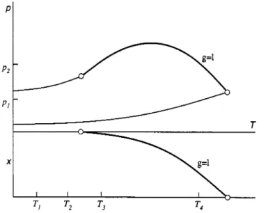
In Figure 9 some ( P J ) and (TJ) sections are shown. The (PJ) sections at T I and T2 have the shape of Figure la. At T3 and T4 component 1 is supercritical and the ( P J ) sections show a binary critical point as in Figure lb. In the T,x-sections the two-phase gl region has a reversed position compared with the P,x-section. Note that the (TJ) section at P2 shows two critical points, which is a consequence of the pressure maximum of the critical curve in the (P,T) projection. These pressure maxima are often found in class 1' systems.
Fig. 9. Class 1' fluid phase behaviour. (a) (PJ) sections at constant T. See Figure 8. (b) (TJ) sections at constant P
.
See Fig. 8.
0 1998 IUPAC, Pure and Applied Chernistry70,2233-2257
Class l P / phase behaviour
Class 1'1 phase behaviour (type I1 according to the classification of van Konynenburg & Scott) has a continuous vapour-liquid critical curve just as in the case of class 1' phase behaviour. In addition, systems of this type show a liquid-liquid critical curve l1 = l2 and a three-phase equilibrium g1112
.
See Fig. 10, which shows the P,T- and Tj-projection of a class 1'1 system. In the (P,T) projection the curves l1 = l2 and g1112 intersect in a UCE g(ll = 12.) In the diagram shown the liquid-liquid critical curve has a positive slope in the (P,T) projection, but this curve can also have a negative slope or a temperature minimum. If not interrupted by the formation of a solid phase, the l1 = l2 curve runs to infinite pressure.Both the l1 = l2 curve and the g1112 curve can be completely hidden by a solid-liquid equilibrium surface, so in practice it may be impossible to distinguish between class 1' phase behaviour and class 1'1 phase behaviour. For instance, in the binary systems of carbon dioxide
+
n-alkanes for carbon number n 6<nc13 type I1 phase behaviour is found (Schneider, 1978). For lower values of n no stable liquid-liquid equilibria are found, but it is very likely that the system carbon dioxide+
n-pentane, for instance, is also ofclass 1'1.T
-
'-
'-
'2'
-AI 1.
Fig. 10. Combined (P,T) and (TJ) projections of class lPZ fluid phase behaviour. ~ : vapour-pressure curves; -: critical curves; - - - - -: three-phase curve; 0: pure component critical point; A: upper critical endpoint.
In Fig. 11 four characteristic (P,x) sections are shown. At low temperature the Pyx-sections show a g1112 equilibrium. At higher pressure than the three-phase pressure the gll and 1112 two-phase regions are found, and at lower pressure the two-phase region g12. With increasing temperature the compositions of the two liquid phases of the g1112 equilibrium approach each other, as can be seen from the (T,x) projection in Fig. 10. At the temperature of the UCE a critical phase l1 = 12 is in equilibrium with a vapour phase and, as a consequence, the gll and g12 regions join in one two-phase region gl, which shows a horizontal point of inflection at the l1 = l2 critical point. At higher temperatures the gl region and the 1112 region are separated by a region of a homogeneous liquid phase. At even higher temperatures the 1112 region shifts to higher pressures and the gl region may detach on the left hand side, as shown in Fig. 9a.
0 1998 IUPAC, Pure and Applied Chemistry70,2233-2257
2252 COMMISSION ON THERMODYNAMICS
X
I g I
X
I I
X X
Fig. 11. Class 1'1 fluid phase behaviour. (PJ) sections at constant T. (a, b) T<T(g(ll = 12)). (c) T = T(g(1l = 12). (d) T(g(1, = l2)<T<T(g = l)x=o) See Fig. 10.
Class '2 phase behaviour
The phase behaviour class 2' systems (type V according to the classification of van Konynenburg & Scott)is is represented by (P,T) and (T,x) projections given in Fig. 12. Characteristic for this type of phase behaviour is a three-phase equilibrium g1112 with a LCE g(ll = 12) and a UCE (g = 11)12, and a discontinuous critical curve.
T
Fig. 12. Combined (P,T) and ( T J ) projections of class 2' fluid phase behaviour. : vapour-pressure curves; : critical curve; : three-phase curve; 0: pure component critical point; A, V: upper and lower critical endpoints.
0 1998 IUPAC, Pure and Applied Chemistry70,2233-2257
The first branch of the critical curve connects the critical point of the more volatile component with the UCE. The second branch runs from the LCE to the critical point of the less volatile component.
Examples of class 2' systems are the systems methane
+
n-hexane (Davenport & Rowlinson, 1963) and ethane+
n-eicosane (Kohn et al., 1966), although there are reasons to believe that these systems are in reality class 2'1 systems (see section on class 2'1 systems).In Fig. 13 four (PJ) sections are shown at temperatures T(g(ll = 12))1TIT((g = 11)12). At lower and at higher temperatures the (P,x) sections are comparable with those of class 1' systems. In Figure 13b a (PJ) section is shown at a temperature between the LCE and the critical point of the more volatile component. This (PJ) section is comparable with Fig. I l a . On lowering the temperature, the composition of the l1 phase and of the l2 phase of the g1112 equilibrium approach each other and the pressure of the 1, = l2 critical point approaches the three-phase pressure. At the temperature of the LCE (see Fig. 13a) the l1 and l2 points of the three-phase equilibrium and the critical point l1 = l2 coincide. The 1112 two-phase region disappears and the gll and g12 two-phase regions join in one gl two-phase region.
The gl region shows a horizontal point of inflection at the l1 = l2 critical point. At higher temperatures than the temperature of Fig. 13b the gll region will detach from the axis x = 0 (Fig. 13c) and at even higher temperatures the composition of the l1 phase and of the vapour phase of the g1112 equilibrium approach each other. At the temperature of the UCE the l1 and g points of the three-phase equilibrium and the g = llcritical point coincide. See Figure 13d. At this temperature the gll two-phase region disappears and the g12 and 1112 two-phase regions again join in one gl two-phase region. Now the gl region shows a horizontal point of inflection at the g = l1 critical point.
X
I
L
X
X
X
Fig. 13. Class 2' fluid phase behaviour fluid. (PJ) sections at constant T. (a) T = T(L = L V). (b) T(g(1, = 12))<T<T(g = l), = o. (c) T<T(g = l), = o<T<T((g = 11)12). (d) T = T((g = 11)12). See Fig. 12.
Class 2'1 phase behaviour
The combined (P,Z') and ( T J ) projections of a class 2'1 system (type IV according to the classification of van Konynenburg & Scott) is given in Fig. 14. In this type of phase behaviour the three-phase equilibrium g1112 consist of two branches. The low-temperature branch shows a UCE g(ll = 12) and is comparable with the g1112 equilibrium that is found in class 1'1 systems. The high-temperature branch
0 1998 IUPAC, Pure and Applied Chemistry70,2233-2257
2254 COMMISSION ON THERMODYNAMICS
shows a LCE g(ll = 1,) and a UCE (g = 11)12 and is comparable with the g1112 equilibrium that is found in class 2' systems. Not many binary class 2'1 systems are known, but for similar reasons as mentioned for class 1'1 phase behaviour it is likely that many systems that are supposed to show class 2' phase behaviour in fact are of class 2'1 and the low-temperature branch of the gll12 equilibrium is masked by the solidification surface. The system carbon dioxide
+
tridecane (Enick et al., 1985; Fall & Luks, 1985) is an example of a system showing class 2'1 fluid phase behaviour.T
Fig. 14. Combined (P,T) and (T,x) projections of class 2'1 fluid phase behaviour. ~ : vapour-pressure curves; -: critical curves; - - - - - - -: three-phase curves; 0: pure component critical point; A, V:
upper and lower critical endpoints.
Since class 1'1 and class 2' phase behaviour is combined in class 2'1 phase behaviour, the (P,x) sections at low temperatures are those of class 1'1 (Fig. 11) and at high temperature those of class 2' (Fig. 13). However phase diagrams at constant temperature can show two separated regions of liquid-liquid immiscibility. An example of a (T,x) section is given in Fig. 15. At this pressure the high-temperature branch of the gll12 curve is intersected in the P,T-projection. The (T,x) section shows three critical points. At low temperature a critical point 11 = 12 is the maximum temperature of a 1112 two-phase region. This kind of critical point is called upper critical solution temperature (UC,). The other 1112 critical point is the minimum temperature of a second 1112 two-phase region, which ends at higher temperature at the 81112 equilibrium. This critical point is called a lower critical solution temperature (LCp). The third critical point is a vapour-liquid critical point g = 12.
I
X
Fig. 15. Class 2'Z fluid phase behaviour. (T,x) section at constant P for: P(LCE)dJdJ(g = 1),=,,. See Fig. 14.
0 1998 IUPAC, Pure and Applied Chernistry70,2233-2257
T
Fig. 16. Combined ( P , Q and (TJ) projections of class 1'1' fluid phase behaviour.
-
:vapour-pressure curves; :- critical curves; - - - -: three-phase curves; 0: pure component critical point; A: upper critical endpoints.Class l c l Z p h a s e behaviour
In class 1'1' phase behaviour (type I11 according to the classification of van Konynenburg & Scott) the two branches of the glllz equilibrium of class 2'1 phase behaviour are combined, and also two of the three branches of the critical curve that are found for class 2'1. Only the UCE (g = 11)12 remains. The (P,T) and (T,x) projection of class 1'1' phase behaviour are given in Fig. 16. In the example shown the branch of the critical curve that runs from high pressure to the critical point of the less volatile component shows a pressure minimum and a pressure maximum. An example of this behaviour is found in the system propane
+
triphenylmethane (de Roo et al., 1995). This branch of the critical c m e can also show a temperature minimum combined with a pressure minimum and a pressure maximum(i.e. carbon dioxide+
tetradecane (Hottovy et al., 1981), or only a temperature minimum (i.e. propane+
water (de Loos et al., 1980) or can have a positive value of (dP/dT) in the critical point of the less volatile component (i.e., He+
Xe (de Swaan Arons & Diepen, 1966)). See Fig. 17. Since in the latter two types of systems two-phase equilibria can exist at higher temperatures than the critical temperature of the less volatile component these equilibria are often referred to as gas-gas equilibria. The system He+
Xe is said to show gas-gas equilibria of the first kind (no minimum critical temperature), the system propane+
watergas-gas equilibria of the second kind (the critical line passes through a minimum in temperature).
0 1998 IUPAC, Pure and Applied Chemistry70,2233-2257