FOUR EDGE-INDEPENDENT SPANNING TREES

FOUR EDGE-INDEPENDENT SPANNING TREES

Alexander Hoyer and

Robin Thomas School of Mathematics Georgia Institute of Technology Atlanta, Georgia 30332-0160, USA

ABSTRACT

We prove an ear-decomposition theorem for 4-edge-connected graphs and use it to prove that for every 4-edge-connected graphGand everyr ∈V(G), there is a set of four spanning trees of Gwith the following property. For every vertex inG, the unique paths back to r in each tree are edge-disjoint. Our proof implies a polynomial-time algorithm for constructing the trees.

March 2017. Revised October 2017.

1Partially supported by NSF under Grant No. DMS-1202640.

2Presented at the 29th Cumberland Conference on Combinatorics, Graph Theory and Computing at Vanderbilt University.

arXiv:1705.01199v3 [math.CO] 21 Nov 2017

1 Introduction

If r is a vertex of a graph G, two subtrees T₁, T₂ of G are edge-independent with root r if each tree containsr, and for eachv ∈V(T₁)∩V(T₂), the unique path in T₁ between rand v is edge-disjoint from the unique path in T₂ between r and v. Larger sets of trees are called edge-independent with root r if they are pairwise edge-independent with root r.

Itai and Rodeh [6] posed the Edge-Independent Tree Conjecture, that for every k-edge- connected graphG and every r∈V(G), there is a set of k edge-independent spanning trees of G rooted at r. Here, we prove the case k = 4 of the Edge-Independent Tree Conjecture.

That is, we prove the following:

Theorem 1. If G is a4-edge-connected graph and r∈V(G), then there exists a set of four edge-independent spanning trees of G rooted at r.

There is a similar conjecture which has been studied in parallel, concerning vertices rather than edges. Ifr is a vertex of G, two subtrees T₁, T₂ ofGare independent with root r if each tree contains r, and for each v ∈ V(T₁)∩V(T₂), the unique path in T₁ between r and v is internally vertex-disjoint from the unique path in T₂ between r and v. Larger sets of trees are called independent with root r if they are pairwise independent with root r.

Itai and Rodeh [6] also posed the Independent Tree Conjecture, that for everyk-connected graph Gand for every r∈V(G), there is a set of k independent spanning trees ofG rooted atr.

The case k = 2 of each conjecture was proven by Itai and Rodeh [6]. The case k = 3 of the Independent Tree Conjecture was proven by Cheriyan and Maheshwari [1], and then independently by Zehavi and Itai [11]. Huck [5] proved the Independent Tree Conjecture for planar graphs (with anyk). Building on this work and that of Kawarabayashi, Lee, and Yu [7], the case k = 4 of the Independent Tree Conjecture was proven by Curran, Lee, and Yu across two papers [2, 3]. The Independent Tree Conjecture is open for nonplanar graphs with k >4.

In 1992, Khuller and Schieber [8] published a later-disproven argument that the Inde- pendent Tree Conjecture implies the Edge-Independent Tree Conjecture. Gopalan and Ra- masubramanian [4] demonstrated that Khuller and Schieber’s proof fails, but salvaged the technique, and proved the case k= 3 of the Edge-Independent Tree Conjecture by reducing it to the case k= 3 of the Independent Tree Conjecture. Schlipf and Schmidt [10] provided an alternate proof of the case k = 3 of the Edge-Independent Tree Conjecture, which does not rely on the Independent Tree Conjecture. The case k= 4 of the Edge-Independent Tree Conjecture is proven here, while the case k > 4 remains open.

By adapting the technique of Schlipf and Schmidt [10], we prove an edge analog of the planar chain decomposition of Curran, Lee, and Yu [2]. We then use this decomposition to create two edge numberings which define the required trees.

The conjectures are related to network communication with redundancy. If Grepresents a communication network, one can wonder if information can be broadcast through the entire network with resistance to edge failures (i.e. it would require ksimultaneous edge failures to disconnect a client from every broadcast). The Edge-Independent Tree Conjecture implies that the absence of edge bottlenecks of size less than k is necessary and sufficient for a redundant broadcast to be possible from any source r. The Independent Tree Conjecture answers the analogous problem where vertex failures are the concern, rather than edge failures.

2 The Chain Decomposition

In this paper, a graph will refer to what is commonly called a multigraph. That is, there may be multiple edges between the same pair of vertices (“parallel edges”) and an edge may connect a vertex to itself (a “loop”). All paths and cycles are simple, meaning they have no repeated vertices or edges. We consider a loop to induce a cycle of length one and a pair of parallel edges to induce a cycle of length two. Also, the presence of a loop increases the degree of a vertex by two. We will use the overline notation H to name specific subgraphs, rather than for the graph complement.

Throughout this section, fix a graph G with |V(G)| ≥ 1 and a vertex r ∈ V(G). We begin by defining a decomposition analogous to the planar chain decomposition in [2].

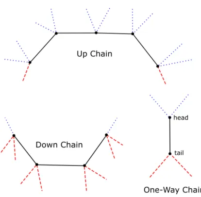
Definition. An up chain of Gwith respect to a pair of edge-disjoint subgraphs (H, H) is a subgraph of G, edge-disjoint from H and H, which is either:

i A path with at least one edge such that every vertex is either r or has degree at least two in H, and the ends are either r or are in H, OR

ii A cycle such that every vertex is either r or has degree at least two in H, and some vertexv is eitherr or has degree at least two inH. We will considerv to be both ends of the chain, and all other vertices in the chain to be internal vertices.

Chains which are paths will be called open and chains which are cycles will be calledclosed, analogous to the standard ear decomposition.

Definition. A down chain of Gwith respect to a pair of edge-disjoint subgraphs (H, H) is an up chain with respect to (H, H).

Definition. A one-way chain of G with respect to the pair of edge-disjoint subgraphs (H, H) is a subgraph of G, induced by an edge e /∈ H ∪H with ends u and v, such that u is either r or has degree at least two in H, and v is either r or has degree at least two in H.

We callu the tail of the chain and v the head.

Definition. Let G₀, G₁, . . . , G_m be a sequence of subgraphs of G. Denote H_i =G₀ ∪G₁∪

· · · ∪Gi−1 and H_i =G_i+1∪G_i+2∪ · · · ∪G_m, so that H₀ and H_m are the null graph. We say that the sequence G₀, G₁, . . . , G_m is a chain decomposition of G rooted atr if:

1. The sets E(G₀), E(G₁), . . . , E(G_m) partitionE(G), AND

2. For i = 0, . . . , m, the subgraph Gi is either an up chain, a down chain, or a one-way chain with respect to the subgraphs (H_i, H_i).

Figure 1: An illustration of an up chain of length 4, a down chain of length 3, and a one-way chain. The red/dashed edges are in earlier chains, while the blue/dotted edges are in later chains.

Definition. Thechain index of e∈E(G), denotedCI(e), is the index of the chain contain- ing e.

Definition. An up chainG_i isminimal if no internal vertex ofG_i is in {r} ∪V (H_i).

Definition. A down chainG_i is minimal if no internal vertex ofG_i is in {r} ∪V H_i . Definition. A chain decomposition is minimal if all of its up chains and down chains are minimal.

Remarks.

1. A minimal up chain is a special case of an ear in the standard ear decomposition.

2. The chain decomposition is symmetric in the following sense. If G₀, G₁, . . . , G_m is a chain decomposition rooted at r, then G_m, Gm−1, . . . , G₀ is a chain decomposition rooted at r, with the up and down chains switched and the heads and tails of one-way chains switched. Throughout this paper, we will refer to this fact as “symmetry”.

3. G₀ is either a closed up chain ending at r or a one-way chain with r as the tail, and G_m is either a closed down chain ending atr or a one-way chain with r as the head.

4. In the planar chain decomposition in [2], up chains and down chains are analogous to the corresponding open chains. The elementary chain is analogous to a one-way chain.

Remark 2. An up chain or down chain may be subdivided into several minimal chains by breaking at the offending internal vertices. These minimal chains may then be inserted consecutively to the decomposition at the index of the old chain. In this way, one can easily obtain a minimal chain decomposition from any chain decomposition.

We will prove Theorem 1 by combining the following results:

Theorem 3. If G is a 4-edge-connected graph and r∈V(G), then G has a chain decompo- sition rooted at r.

Theorem 4. SupposeG is a graph with no isolated vertices. IfG has a chain decomposition rooted at some r ∈ V(G), then there exists a set of four edge-independent spanning trees of G rooted at r.

3 Preliminary Results

While not needed for our main results, the following proposition demonstrates how the chain decomposition fits in with the various decompositions used in other cases of the Independent Tree Conjecture and Edge-Independent Tree Conjecture. A partial chain decomposition and its complement are “almost 2-edge-connected” in the following sense.

Proposition 5. SupposeG₀, G₁, . . . , G_m is a chain decomposition of a graph G rooted at r.

Then for i = 1, . . . , m, H_i and H_i−1 are connected. Further, if e is a cut edge of H_i (resp.

Hi−1), theneinduces a one-way chain and one component ofH_i−e (resp. Hi−1−e) contains one vertex and no edges.

Proof. By symmetry, we need only prove the result for the H_i’s. The connectivity follows from the fact that every type of chain is connected and contains at least one vertex in an earlier chain.

Suppose e is a cut edge of some H_i. Since e is an edge in H_i, we have CI(e) < i and H_CI(e) ⊂ Hi. We also know that H_CI(e) is connected by the previous paragraph. Then e cannot be part of an up chain, or else e would be part of a cycle formed by the chainGCI(e)

and a path in H_CI(e) between the ends of G_CI(e) (if G_CI(e) is open; else the chain itself is a cycle). Also,e cannot be part of a down chain, or else e would be part of a cycle formed by e and a path in H_CI(e) between the ends of e. Therefore, e induces a one-way chain.

Let C be the component of H_i−e not containingr, and suppose for the sake of contra- diction that C contains an edge. Let e⁰ be an edge ofC with minimal chain index. Consider G_CI(e⁰₎, the chain containing e⁰. Regardless of the chain type, some vertices in V(G_CI(e⁰₎) are incident to at least two edges inH_CI(e⁰₎ ⊂H_i since r /∈C, so one of these edges is note.

This contradicts the minimality ofCI(e⁰).

The next lemma and its corollary will allow us to ignore the possibility of loops in the graph when convenient.

Lemma 6. SupposeG₀, G₁, . . . , G_m is a chain decomposition ofG rooted atr. If v 6=r is in H_i (resp H_i), then v is incident to a non-loop edge in H_i (resp H_i). If v has degree at least two in Hi (resp. Hi), then v is incident to two distinct non-loop edges in Hi (resp. Hi).

Proof. Note that the second claim in the lemma implies the first, since a loop increases the degree of a vertex by 2, so it suffices to prove the second claim in the lemma.

Suppose v is incident to a loop, which by symmetry we may assume is in H_i. Of all loops incident to v, choose the one with minimal chain index j < i. Consider the chain classification ofG_j. The chain definitions all coincide for a loop, and require thatv(6=r) has degree at least two in H_j. By the minimality of j, v is not incident to any loops in H_j. It follows that v is incident to two distinct non-loop edges inH_j ⊂H_i.

Corollary 7. Suppose G₀, G₁, . . . , G_m is a chain decomposition of G rooted at r, and e ∈ E(Gi) is a loop. Then G0, G1, . . . , Gi−1, Gi+1, . . . , Gm is a chain decomposition of G− e rooted at r. Further, if G has no isolated vertices, then G−e has no isolated vertices.

Proof. The first claim follows from the preceding lemma. For the second, observe that ifeis the only edge incident to its end, then it fails the conditions for every chain definition.

Next, we prove the following useful fact about minimal chain decompositions.

Lemma 8. Suppose G is a graph with no isolated vertices, G0, G1, . . . , Gm is a minimal chain decomposition of G rooted at r, and v ∈V(G) with v 6=r. Then there are indices i, j so that v has degree exactly two in H_i and H_j.

Proof. By symmetry, we need only find i. Since G has no isolated vertices, v is in some chain. Consider the chain G_i0 containingv so that i₀ is minimal. Note that v /∈V(H_i0).

If G_i0 is an up chain, then v is an internal vertex of G_i0 since v /∈ V(H_i0), so v has degree two inG_i0 and degree at least two inH_i0. Therefore H_i0 is not null, soi₀ < m. Then i=i₀+ 1 completes the proof.

The chain G_i0 is not a down chain since v /∈V(H_i0).

So we may assume thatGi0 is a one-way chain, andv must be the head sincev /∈V(Hi0).

Therefore v has degree at least two inHi0, so we may consider the next chain to contain v, say G_i1. Note that v has degree one inH_i1 by the definition of i₁.

If G_i1 is an up chain, then it is open and v is an end of the chain, since the chain decomposition is minimal and v has degree one in H_i1. The chain G_i1 is not a down chain sincev has degree one inH_i1. If G_i1 is a one-way chain, then v is the head since v(6=r) does not have degree at least two in H_i1. In all cases,v has degree one inG_i1 and degree at least two in H_i1. Therefore H_i1 is not null, so i₁ < m. Then i=i₁+ 1 completes the proof.

Finally, we show that the chain decomposition implies a minimum degree result.

Lemma 9. Suppose G is a graph with no isolated vertices, G₀, G₁, . . . , G_m is a chain de- composition of G rooted at r, and v ∈V(G) with v 6=r. Then v has degree at least 4.

Proof. By Corollary 7, we may assume that there are no loops in G. If v is in an up chain G_i, then v has degree at least 2 in H_i, and either degree 2 in G_i (if v is internal) or degree at least 1 in Gi and degree at least 1 in Hi (if v is an end). Either way, v has degree at least 4 in G. By symmetry, the same is true if v is in a down chain.

So we may assume that the only chains containing v are one-way chains. SinceG has no isolated vertices, there is at least one such chain G_j. Then v has degree 1 in G_j and degree at least 2 in H_j (if v is the tail) or H_j (if v is the head). We conclude that v has degree at least 3 in G.

Assume for the sake of contradiction that v does not have degree at least 4. Then v has degree 3 and is in exactly three one-way chains, say G_{`1</sub>, G<sub>`2}, G<sub>`3</sub> with `₁ < `<sub>2</sub> < `₃.

Consider G_{`2</sub>. Since we know all of the chains containing v, we can say that v has degree 1 in H<sub>`2} and degree 1 in H_{`2</sub>. This contradicts the definition of a one-way chain, as v can be neither the head nor the tail of the chain G<sub>`2}. We conclude that v has degree at least 4 as desired.

Remark. If |V(G)| ≥ 2 in addition to G having a chain decomposition and no isolated vertices, then G is 4-edge-connected sor has degree at least 4 as well. However, we will not need this result, and it will follow from Corollary 12.

4 The Mader Construction

We will adapt the strategy of Schlipf and Schmidt [10] in order to construct a chain decom- position. In particular, we will use a construction method for k-edge-connected graphs due to Mader [9]. We limit our description of the construction to the needed case k = 4, since the method is more complicated for odd k.

Definition. A Mader operation is one of the following operations:

1. Add an edge between two (not necessarily distinct) vertices.

2. Consider two distinct edges, say e1 with ends x,y and e2 with ends z,w, and “pinch”

them as follows. Delete the edges e1 and e2, add a new vertex v, then add the new edges e_x, e_y, e_z, e_w with one end v and the other end x, y, z, w respectively. While e₁ ande₂ must be distinct, the endsx, y, z, wneed not be. In this case,vwill have parallel edges to any repeated vertex.

Theorem 10 ([9, Corollary 14]). A graph G is 4-edge-connected if and only if, for any r ∈V(G), one can construct G in the following way. Begin with a graph G⁰ consisting of r and one other vertex ofG, connected by four parallel edges. Then, repeatedly perform Mader operations to obtain G.

Remark. Mader does not explicitly state that one can include a fixed vertex r inG⁰, but it follows from his work. His proof starts withG, and then reverses one of the Mader operations while maintaining 4-edge-connectivity. An edge can be deleted unlessGis minimally 4-edge- connected, in which case he finds two vertices of degree 4 in his Lemma 13. He then shows that any degree 4 vertex can be “split off” (the reverse of a pinch) in his Lemma 9, so we can always split off a vertex not equal to r.

5 Proof of Theorem 3

Due to Theorem 10, it suffices to prove that a chain decomposition can be maintained through a Mader operation. The decomposition in the starting graph G⁰ is as follows. Two of the edges form a closed up chain. The remaining two edges form a closed down chain.

Suppose the graph G⁰ is obtained from the graph G by a Mader operation, with both graphs 4-edge-connected. Assume that we have a chain decompositionG₀, G₁, . . . , G_m ofG.

By Remark 2, we may assume that we have a minimal chain decomposition. We wish to create a new chain decomposition ofG⁰.

5.1 Adding an Edge

Suppose G⁰ is obtained from G by adding an edge with ends u, v. If one of the ends is the rootr, we can classify the new edge as a one-way chain with tailrat, say, the very beginning of the chain decomposition. The head must have at least two incident edges in later chains, since all chains are later.

If neither end is r, choose the minimal index i such that u or v has degree exactly two in Hi, guaranteed to exist by Lemma 8. Note that i ≥ 1 since H0 is null. Without loss of generality,uhas degree exactly two inH_i. By the definition ofi,v has degree at most two in H_i, and therefore degree at least two inHi−1. We classify the new edge as a one-way chain with tail u and head v, between the chains Gi−1 and G_i.

We consider the impact of these changes on other chains in the graph. A new chain was added, but none of the other chains changed index relative to each other. Vertices may have increased degree in theH_i’s or theH_i’s due to the new edge, but increasing degree does not invalidate any chain types. Note that some chains may no longer be minimal, so the new chain decomposition in G⁰ is not necessarily minimal.

5.2 Pinching Edges

Suppose G⁰ is obtained from G by pinching the edges e₁ with ends x, y and e₂ with ends z, w, replacing them with edges e_x, e_y, e_z, e_w. We will use the notation J₁ =G_CI(e1) =P_xe₁P_y for the chain containing e₁, where P_x is the subpath between x and an end of J₁ so that e₁ ∈/ E(P_x), and P_y is defined similarly. Note that P_x (resp. P_y) may have no edges if x (resp. y) is an end of J₁. In the same way, we will use the notation J₂ =G_CI(e2) =P_ze₂P_w for the chain containing e₂.

We now prove several claims to deal with all possible chain classification and chain index combinations for J₁ and J₂.

Claim 1. If CI(e₁) =CI(e₂), then G⁰ has a chain decomposition rooted at r.

Proof. If CI(e₁) = CI(e₂), then J₁ = J₂. Without loss of generality, e₁ ∈ E(P_z) and e₂ ∈E(P_y), so that the chain can be written asJ₁ =J₂ =P_xe₁(P_y∩P_z)e₂P_w (whereP_y∩P_z may have no edges if y=z). Recall thate₁ and e₂ are distinct, so J₁ =J₂ is not a one-way chain.

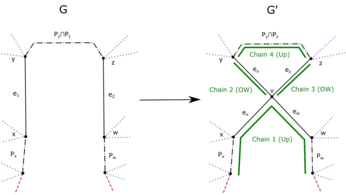
By symmetry, we may assumeJ₁ =J₂ is an up chain. InG⁰, we replace the chainJ₁ =J₂ with the following chains (in the listed order); see Figure 2 for an illustration:

1. P_xe_xe_wP_w. This is an up chain. Since the edgese_y and e_z have not yet been used, the new vertex v is incident to two edges in later chains.

2. e_y. This is a one-way chain with tail v and head y. The tail v is incident to two edges in earlier chains, namelye_x and e_w. The heady is incident to two edges in later chains since it was an internal vertex in the old up chainJ₁ =J₂.

3. ez. This is a one-way chain with tailv and head z. The tail v is incident to two edges in earlier chains, namelye_x and e_w. The headz is incident to two edges in later chains since it was an internal vertex in the old up chainJ₁ =J₂.

4. (P_y ∩P_z). Only add this chain if P_y ∩P_z contains an edge. This is an up chain. The new ends y, z are each incident to an edge in an earlier chain (e_y and e_z, respectively) and are each incident to two edges in later chains since they were interior vertices of the old up chain J₁ =J₂.

We consider the impact of these replacements on other chains in the graph. We inserted most of the edges of the old chain J₁ = J₂ at the same chain index CI(e₁) = CI(e₂), preventing any changes. The exception is the pinched edges e₁ and e₂ which were deleted, but the ends each received new incident edges e_x, e_y, e_z, e_w inserted at the same chain index CI(e₁) = CI(e₂). Thus, we have maintained the chain decomposition. This proves Claim 1.

Without loss of generality, we assume the following for the remainder of the proof:

• CI(e₁)< CI(e₂).

• IfJ₁ is a one-way chain, then x is the tail and y the head.

• IfJ2 is a one-way chain, then z is the tail and w the head.

Figure 2: An illustration of the procedure in Claim 1. The original up chain J₁ =J₂ is on the left, while its replacements in G⁰ are on the right. The red/dashed edges are in earlier chains than J₁ = J₂, while the blue/dotted edges are in later chains than J₁ = J₂. The black/dashed-and-dotted segments represent paths which may have any length (including 0).

Claim 2. Suppose that either J₁ is a one-way chain whose head y has degree one in H_CI(e2), or J₂ is a one-way chain whose tail z has degree one in H_CI(e1). Then G⁰ has a chain decomposition rooted at r.

Proof. By symmetry, we may assume J1 is a one-way chain whose heady has degree one in H_CI(e2).

First, we replace J₁ with e_x. This is a one-way chain with tailx and head v. The tail x was the tail of the old one-way chain J₁. The headv has two (in fact three) incident edges in later chains, namely e_y, e_z, e_w.

• Case 1: J2 is an up chain. Since y has degree one in H_CI(e2), if J2 is closed then y is not the end ofJ2. By swappingz andw if necessary, we may assume that yis not the end of J₂ inP_z. Thus, the end of J₂ in P_z is still either r or incident to an edge in an earlier chain, despite having not placed e_y yet. We use the edges of J₂ and e_y, e_z, e_w to construct chains at the index CI(e₂) as follows:

1. Pzez. This is an up chain. The new end, v, has one incident edge in an earlier chain (ex) and two incident edges in later chains (ey,ew). By assumption, the old

end inP_z is still eitherr or incident to an edge in an earlier chain.

2. e_y. This is a one-way chain with tail v and head y. The tail v is incident two edges in earlier chains (e_x, e_z). The head y is either r or incident to two edges in later chains, since y has degree one inH_CI(e2) by assumption.

3. e_w. This is a one-way chain with tail v and head w. The tail v has two (in fact three) incident edges in earlier chains (e_x, e_y, e_z). The head w is either r or incident to two edges in later chains, since it was part of the old up chainJ₂. 4. P_w. Only add this if P_w contains an edge. This is an up chain. The new end,

w, has one incident edge in an earlier chain (e_w) and two incident edges in later chains since it was an internal vertex of the old up chainJ₂. Since we placed e_y above, the end ofJ₂ inP_w has is either ror incident to an end in an earlier chain, even if the end is y.

• Case 2: J₂ is a down chain. Since y has degree one in H_CI(e2), y /∈ V(J₂), so each vertex of J₂ is still either r or incident to two edges in earlier chains, despite having not placed e_y yet. We use the edges of J₂ and e_y, e_z, e_w to construct chains at the index CI(e₂) as follows:

1. P_w. Only add this if P_w contains an edge. This is a down chain. The new end, w, has one incident edge in a later chain (e_w) and two incident edges in earlier chains since it was an internal vertex of the old down chain J₁.

2. e_w. This is a one-way chain with tail w and head v. The tail w is either r or incident to two edges in earlier chains since it was part of the old down chainJ₂. The head v is incident to two edges in later chains (e_y,e_z).

3. P_ze_z. This is a down chain. The new end, v, has one incident edge in a later chain (e_y) and two incident edges in earlier chains (e_x, e_w).

4. e_y. This is a one-way chain with tail v and head y. The tail v has two (in fact three) incident edges in earlier chains (ex, ez, ew). The head y is either r or incident to two edges in later chains since y has degree one in HCI(e2) and y /∈V(J₂) by assumption, so y has degree at least three in H_CI(e2) unless it is r.

• Case 3: J₂ is a one-way chain. Since y has degree one in H_CI(e2), y 6= z so the tail z is still either r or incident to two edges in earlier chains, despite having not placed e_y yet. We use the edges ey, ez, ew to construct chains at the index CI(e2) as follows:

1. e_z. This is a one-way chain with tail z and head v. The tail z is either r or incident to two edges in earlier chains as discussed above. The headv is incident to two edges in later chains (e_y, e_w).

2. e_w. This is a one-way chain with tail v and head w. The tail v is incident to two edges in earlier chains (e_x, e_z). The head wis either ror incident to two edges in later chains since it was the head ofJ₂.

3. e_y. This is a one-way chain with tail v and head y. The tail v has two (in fact three) incident edges in earlier chains (e_x, e_z, e_w). The head y is either r or incident to two edges in later chains since y has degree one in H_CI(e2) and y /∈V(J₂) by assumption, so y has degree at least three in H_CI(e2) unless it is r.

We consider the impact of these replacements on other chains in the graph. As before, most of the edges of the old chainsJ₁ and J₂ were inserted at the same chain indicesCI(e₁) and CI(e₂) respectively, preventing any changes. The pinched edgese₁ and e₂ were deleted, but the ends x, z, w each received new incident edges e_x, e_z, e_w inserted at the same chain indices (CI(e₁), CI(e₂), and CI(e₂) respectively). However, e_y was inserted at a different chain index than the deleted edge e₁ since e₁ was at CI(e₁) while e_y is at CI(e₂). By the claim assumptions, y has degree one in H_CI(e2), so there are no chains containing y between CI(e1) andCI(e2), and so no chains were affected by the change. Thus, we have maintained the chain decomposition. This proves Claim 2.

We may now assume the following for the remaining cases:

• IfJ₁ is a one-way chain, then y has degree at least two in H_CI(e2).

• IfJ₂ is a one-way chain, then z has degree at least two in H_CI(e1).

We also make the following conditional definitions, which will aid in distinguishing the remaining cases:

• If J₁ is a one-way chain and y is not in H_CI(e1), then define the minimal index i such that y ∈ V(Gi) and CI(e1)< i < CI(e2). Since i is minimal, y has degree one in Hi

(incident only to the pinched edge e1). From this and the fact that Gi is a minimal chain, it follows that eithery is one of two distinct ends of the up chainG_i, or yis the head of the one-way chain G_i which is not a loop.

• If J₂ is a one-way chain and z is not inH_CI(e2), then define the maximal index j such that z ∈V(Gj) and CI(e1)< j < CI(e2). Sincej is maximal, z has degree one in Hj

(incident only to the pinched edge e2). From this and the fact that Gj is a minimal

chain, it follows that either z is one of two distinct ends of the down chain G_j, or z is the tail of the one-way chain G_j which is not a loop.

Claim 3. Suppose that either one of i, j is not defined, or i < j. Then G⁰ has a chain decomposition rooted at r.

Proof. The chains replacing J₁ will have indices adjacent to CI(e₁) and i (if it is defined).

Likewise, the chains replacingJ₂ will have indices adjacent to CI(e₂) andj (if it is defined).

Thus, by the assumptions of this claim, the chains replacing J1 will have lower chain index than the chains replacing J₂. This fact will be needed when confirming that the new chains are valid. We begin by replacing J₁ as follows:

• Case 1: J₁ is an up chain. We replace it with P_xe_xe_yP_y. This is an up chain. The new vertex v has two incident edges in later chains, namely e_z and e_w.

• Case 2: J₁ is a down chain. We replace it with the following chains (in the listed order):

1. P_x. Only add this chain if P_x contains an edge. This is a down chain. The new end x has an incident edge in a later chain, namelye_x.

2. Py. Only add this chain if Py contains an edge. This is a down chain. The new end y has an incident edge in a later chain, namely e_y.

3. e_x. This is a one-way chain with tail x and head v. The tail x is either r or incident to two edges in earlier chains since it was in the old down chainJ₁. The headv has two incident edges in later chains, namely e_z and e_w.

4. e_y. This is a one-way chain with tail y and head v. The tail y is either r or incident to two edges in earlier chains since it was in the old down chainJ1. The headv has two incident edges in later chains, namely e_z and e_w.

• Case 3: J₁ is a one-way chain whose head y is in H_CI(e1). We replace it with the following chains (in the listed order):

1. e_x. This is a one-way chain with tail xand head v. The tail xwas the tail of the old one-way chain J₁. The head v has two (in fact three) incident edges in later chains, namely e_y, e_z, e_w.

2. e_y. This is an up chain. The vertex y is either r or incident to two edges in later chains since it was the head of the old one-way chain J₁, and it has an incident edge in an earlier chain by assumption. The vertex v has two incident edges in

• Case 4: J₁ is a one-way chain whose head y is not in H_CI(e1). Then i is defined as above.

First, we replace J₁ with e_x. This is a one-way chain with tail xand head v. The tail xwas the tail of the old one-way chainJ1. The head v has two (in fact three) incident edges in later chains, namelyey, ez, ew.

– Subcase 1: yis one of two distinct ends of the up chainG_i. Replace G_i with G_ie_y. This is an up chain. Since G_i was a path andv is a new vertex, this new chain is a path. The new end v is adjacent to one edge in an earlier chain (e_x) and two edges in later chains (ez and ew).

– Subcase 2: y is the head of the one-way chain G_i which is not a loop. Then y is not required to be inH_i forG_i to be a valid chain. In fact,y is not required to be in any of H₀, H₁, . . . , H_i by the definition of i and the assumptions of this case.

Thus, we can leaveGi as is and insert the chainey immediately after Gi. This is an up chain. The vertex y is incident to an edge in the previous chain Gi, and is eitherr or incident to two edges in later chains since it is the head of G_i. The vertex v is adjacent to one edge in an earlier chain (e_x) and two edges in later chains (e_z and e_w).

The procedure for replacing J2 is symmetric, by following the above steps in the reversed chain decomposition.

We consider the impact of these replacements on other chains in the graph. In most cases, we replaced the old chainJ₁ with new chains inserted at the same chain indexCI(e₁), preventing any changes. The pinched edge e₁ was deleted, but the end x received a new incident edge e_x at the same chain index CI(e₁). In Cases 1-3, the same is true for y. In Case 4, y received a new incident edge e_y either at or immediately after the chain index i.

However, by the definition of i and the claim assumptions, no chains were affected by the new chain index except G_i, which was specifically considered and shown to be valid in Case 4. By similar arguments, the changes caused by replacing J₂ also did not invalidate any chains. Thus, we have maintained the chain decomposition. This proves Claim 3.

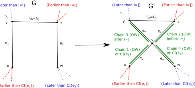
Claim 4. Suppose that both of i, j are defined andi=j. ThenG⁰ has a chain decomposition rooted at r.

Proof. Recall thatG_i is either an up chain or a one-way chain with heady, andG_j is either a down chain or a one-way chain with tail z. Since i =j, we conclude that G_i =G_j must be a one-way chain with tail z and head y, and y 6= z since i and j are defined. We can

replaceJ₁ and J₂ with the following chains, in the listed order. The first two will be placed immediately before indexi=j, and the last two immediately after indexi=j; see Figure 3 for an illustration:

1. e_x. This is a one-way chain with tail x and head v. The tail x was the tail of the old one-way chain J₁ and we are placing this chain after index CI(e₁). The head v has two (in fact three) incident edges in later chains, namely e_y, e_z, e_w.

2. e_z. This is a one-way chain with tail z and head v. By the definition of j, the tail z is either r or incident to two edges in earlier chains than G_j, and we are placing this chain immediately before index j. The head v has two incident edges in later chains, namely e_y and e_w.

3. e_y. This is a one-way chain with tailv and head y. The tailv has two incident edges in earlier chains, namelye_xande_z. By the definition ofi, the headyis eitherror incident to two edges in later chains than G_i, and we are placing this chain immediately after index i.

4. e_w. This is a one-way chain with tail v and head w. The tailv has two (in fact three) incident edges in earlier chains, namely e_x, e_y, e_z. The head w was the head of the old one-way chain J₂, and we are placing this chain before CI(e₂).

We consider the impact of these replacements on other chains in the graph. The deleted edge e1 was replaced by two edges with chain index greater than CI(e1), so we must be careful. The edge ex was inserted before indexi, butxhad degree at least two inHCI(e1), so losing a degree in laterH subgraphs will not invalidate any chains. The edgee_y was inserted immediately after indexi, so by the definition ofi, the only chain affected isG_i. SinceG_i has y as a head, losing a degree in H_i will not invalidate the chain. By a symmetric argument, the changes caused by e_z and e_w do not invalidate any chains. This proves Claim 4.

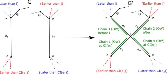
Claim 5. Suppose that both ofi, j are defined, andi > j. ThenG⁰ has a chain decomposition rooted at r.

Proof. We can replace J₁ and J₂ with the following chains, at the indicated chain indices;

see Figure 4 for an illustration:

1. e_x. Add this chain at index CI(e₁). This is a one-way chain with tail x and head v.

The tail x was the tail of the old one-way chain J₁ and we are placing this chain at indexCI(e1). The head v has two (in fact three) incident edges in later chains, namely

Figure 3: An illustration of the procedure in Claim 4. The original chains J₁ and J₂ are on the left, while their replacements in G⁰ are on the right. The red/dashed edges are in earlier chains, while the blue/dotted edges are in later chains, with the particular meanings of “earlier” and “later” in the corresponding labels.

2. e_z. Add this chain immediately afterG_j. This is a one-way chain with tailz and head v. By the definition of j, the tailz is either r or incident to two edges in earlier chains than G_j, and we are placing this chain after index j. The head v has two incident edges in later chains, namelye_y and e_w.

3. ey. Add this chain immediately before Gi. This is a one-way chain with tail v and head y. The tail v has two incident edges in earlier chains, namely e_x and e_z. By the definition of i, the head y is either r or incident to two edges in later chains than G_i, and we are placing this chain before index i.

4. e_w. Add this chain at index CI(e₂). This is a one-way chain with tail v and head w. The tail v has two (in fact three) incident edges in earlier chains, namely e_x, e_y, e_z. The head w was the head of the old one-way chain J₂, and we are placing this chain at index CI(e₂).

We consider the impact of these replacements on other chains in the graph. The edge e₁ was deleted, but x received a new incident edge e_x at the same chain index CI(e₁). The edge e_y was inserted before indexi, but the index is still smaller than i, so by the definition

Figure 4: An illustration of the procedure in Claim 5. The original chains J₁ and J₂ are on the left, while their replacements in G⁰ are on the right. The red/dashed edges are in earlier chains, while the blue/dotted edges are in later chains, with the particular meanings of “earlier” and “later” in the corresponding labels. The black/dashed-and-dotted segments represent paths which may have any length (including 0).

ofi, no chains are affected. By a symmetric argument, the changes caused by e_z ande_w also do not invalidate any chains. This proves Claim 5.

The claims cover all possibilities of pinching edges. The proof of Theorem 3 is complete.

The proof also implies a polynomial-time algorithm to construct a chain decomposition.

6 Proof of Theorem 4

Assume that we have a chain decomposition G₀, G₁, . . . , G_m of G. By Remark 2, we may assume that the chain decomposition is minimal. We will adapt the strategy of Curran, Lee, and Yu [3] to prove Theorem 4. In particular, we will construct two partial numberings of the edges ofG using the chain decomposition. We will then construct four spanning trees in two pairs, with one pair associated with each numbering. Within each pair, paths back to the root r will be monotonic in the associated numbering to ensure independence. Between pairs, paths back to the root r will be monotonic in chain index to ensure independence.

Using Corollary 7, we may assume that there are no loops in G. By Lemma 8, for each vertex v 6= r, there are two distinct non-loop edges incident to v whose chain indices are strictly smaller than the chain index of any other edge incident tov. Likewise there are two distinct edges whose chain indices are strictly larger than the chain index of any other edge

Definition. For each vertex v 6= r, the two f-edges of v are the two incident edges with the lowest chain index. Similarly, the two g-edges of v are the two incident edges with the highest chain index.

Remark 11. By the definition of a down chain, the edges of down chains are never f-edges.

Likewise, by the definition of an up chain, the edges of up chains are never g-edges.

Next, we will iteratively define a numbering f, which will assign distinct values in R to all edges in up chains and one-way chains. Here, two “consecutive” edges in a chain will refer to two edges in the chain which are incident to an internal vertex of the chain, so the two edges incident to the end of a closed chain are not consecutive, despite being adjacent.

We begin by numbering the edges inE(G₀), and then number the edges of each up chain and one-way chain in order of chain index. When we reach a chainG_i, we may assume that all edges in E(H_i) belonging to up chains and one-way chains have been numbered, which includes allf-edges in E(H_i) by Remark 11. We use the following procedure to number the edges inE(G_i):

• If G_i is a closed up chain containing r, then number the edges in E(G_i) so that the values change monotonically between consecutive edges in the chain. The particular numbers used are arbitrary.

• If G_i is a closed up chain not containing r, then both f-edges of the common end have already been numbered. Call these two f-edges numbering edges of G_i. Say the numbering edges of G_i havef-values a and b. Number the edges in E(G_i) so that the values change monotonically between consecutive edges in the chain, and all values are between a and b.

• If G_i is an open up chain containing r, then r is an end and the other end is some u6=r. At least one f-edge of u has already been numbered. Choose an f-edge which has already been numbered and call it a numbering edge of G_i. Say that a is the f-value of the numbering edge. Number the edges in E(G_i) so that the values increase between consecutive edges in the chain when moving from u to r, and all values are larger than a.

• IfG_iis an open up chain not containingr, then at least onef-edge of each end has been numbered. If the ends are uand v, we can choose two distinct edges e_u, e_v ∈E(H_i) so that e_u is an f-edge of u and e_v is an f-edge of v. We can choose these two distinct edges because otherwise, the only f-edge of u or v in E(Hi) would be a single edge betweenuandv, and thenHi would not be connected. Call the edgeseu, ev numbering

edges of G_i. Without loss of generality, f(e_u) = a < b =f(e_v). Number the edges in E(G_i) so that the values increase between consecutive edges in the chain when moving fromu to v, and all values are betweena and b.

• IfG_i is a one-way chain whose tail is r, then number the edge of G_i arbitrarily.

• If G_i is a one-way chain whose tail is not r, then both f-edges of the tail are already numbered, say with f-values a and b. Number the edge of G_i between a and b.

We symmetrically define a numbering g, which assigns distinct values in R to the edges of down chains and one-way chains, by using the above procedure in the reversed chain decomposition.

We are finally ready to construct the trees. Define the subgraphsT₁, T₂, T₃, T₄ as follows.

For each v 6=r, consider the two f-edges ofv. Assign the edge with the lowerf-value to T₁ and the edge with the higher f-value to T₂. Similarly, consider the twog-edges ofv. Assign the edge with the lower g-value to T3 and the edge with the higher g-value toT4.

Several properties of T₁, T₂, T₃, T₄ will follow from the following claim.

Claim. For anyv 6=r, consider the edgee₁ assigned to T₁ atv. Let v⁰ be the other end ofe₁. If v⁰ 6=r, let e⁰₁ be the edge assigned to T₁ at v⁰. Then CI(e⁰₁)≤CI(e₁) and f(e⁰₁)< f(e₁).

Proof. Lete₂ be the edge assigned toT₂ atv. The edgee₁ is not in a down chain by Remark 11. We break into two cases.

• Suppose e₁ is in an up chain G_i. Since the chain decomposition is minimal and v⁰ ∈ V(G_i), its f-edges are either in E(G_i), or else have chain index less thani. In either case, CI(e⁰₁)≤i=CI(e₁) as desired.

Note that e₂ is either in E(G_i), or else is the numbering edge of G_i at the end v. By the numbering procedure, we know that f(e₁) is between f(e₂) and thef-value of one of the f-edges of v⁰, say e^∗. By the definition of T₁, f(e₁) < f(e₂), so it follows that f(e^∗)< f(e₁). Again by the definition ofT₁,f(e⁰₁)≤f(e^∗), sof(e⁰₁)< f(e₁) as desired.

• Supposee₁ induces a one-way chainG_i. Sincee₁ is anf-edge,v has degree at most one inH_i, so v must be the head of G_i. Then v⁰ is the tail ofG_i, so the f-edges ofv⁰ have chain indices smaller thani, which means e⁰₁ 6=e₁ and CI(e⁰₁)< CI(e₁) as desired.

From the numbering procedure, we know thatf(e₁) is between thef-values of the two f-edges of v⁰, with f(e⁰₁) being the smaller by the definition of T₁. So, f(e⁰₁) < f(e₁) as desired.

In both cases we have CI(e⁰₁)≤CI(e₁) and f(e⁰₁)< f(e₁). This proves the claim.

With the claim proven, it follows that the edges assigned to T₁ are all distinct, there are no cycles inT₁, and following consecutive edges assigned to T₁ produces a path which is decreasing in chain index, strictly decreasing in f-value, and can only end at r. Thus, T1 is connected and is a spanning tree of G. A similar argument shows that T2 is a spanning tree of G where paths to r are decreasing in chain index and strictly increasing in f-value. Due to the opposite trends in f-values, T₁ and T₂ are edge-independent with root r.

By symmetry, we obtain analogous results for T₃ and T₄. It remains to show that a tree from {T₁, T₂} and a tree from {T₃, T₄} are edge-independent. The paths back to r from a vertex v 6=r are decreasing in chain index in one tree and increasing in chain index in the other tree, but not strictly. The first edges in these paths are an f-edge and a g-edge of v, respectively. By Lemmas 8 and 9, there is a positive difference in chain index between these initial edges, so the paths are in fact edge-disjoint. The proof of Theorem 4 is complete. The proof also implies a polynomial-time algorithm to construct the edge-independent spanning trees.

7 Summary of Results

With Theorems 3 and 4 proven, we obtain Theorem 1. In fact, we can examine the argument more carefully to extract a stronger, summarizing result.

Corollary 12. Suppose G is a graph with no isolated vertices and V(G) ≥ 2. Then the following statements are equivalent.

1. G is 4-edge-connected.

2. There exists r ∈V(G) so that G has a chain decomposition rooted at r.

3. For all r∈V(G), G has a chain decomposition rooted at r.

4. There exists r∈V(G) so that G has four edge-independent spanning trees rooted at r.

5. For all r∈V(G), G has four edge-independent spanning trees rooted at r.

Proof. Theorem 3 gives us (1)⇒(3). Theorem 4 gives us (2)⇒(4) and (3)⇒(5). Trivially, we have (3)⇒(2) and (5)⇒(4). Therefore, we need only show (4)⇒(1).

Assume for the sake of contradiction that G has four edge-independent spanning trees rooted at some r ∈ V(G), but is not 4-edge-connected. Suppose S ⊆ E(G) is an edge cut with|S|<4. Consider a vertex v in a component ofG−S not containingr. Using the paths

in each of the edge-independent spanning trees, we find that there exist four edge-disjoint paths between v and r. This contradicts the existence of S.

References

[1] J. Cheriyan and S. N. Maheshwari, Finding Nonseparating Induced Cycles and Inde- pendent Spanning Trees in 3-Connected Graphs, J. Algorithms 9 (1988), 507–587.

[2] S. Curran, O. Lee, X. Yu, Chain Decompositions of 4-Connected Graphs, SIAM J.

Discrete Math 19(4)(2005), 848–880.

[3] S. Curran, O. Lee, X. Yu, Finding four independent trees, SIAM J. Comput., 35(5) (2006), 1023–1058.

[4] A. Gopalan and S. Ramasubramanian, On constructing three edge independent spanning trees, unpublished. Available at

http://citeseerx.ist.psu.edu/viewdoc/download?doi=10.1.1.442.3598&rep=rep1&type=pdf.

[5] A. Huck, Independent trees in graphs, Graphs and Combinatorics 10 (1994), 29–45.

[6] A. Itai and M. Rodeh, The multi-tree approach to reliability in distributed networks, Proceedings 25th Annual IEEE Sympos. on Fund. of Comput. Sci. (1984), 137–147.

[7] K. Kawarabayashi, O. Lee, X. Yu, Non-Separating Paths in 4-Connected Graphs, Ann.

Comb. 9 (2005), 47–56.

[8] S. Khuller and B. Schieber, On Independent Spanning Trees, Information Processing Letters 42 (1992), 321–323.

[9] W. Mader, A reduction method for edge-connectivity in graphs, Advances in Graph Theory 3 (1978), 145-164.

[10] L. Schlipf and J. M. Schmidt, Edge-Orders, Proceedings 44th Intl. Colloq. on Automata, Languages, and Programming (2017), 75:1–75:14.

[11] A. Zehavi and A. Itai, Three tree-paths, J. Graph Theory 13 (1989): 175–188.

This material is based upon work supported by the National Science Foundation. Any opinions, findings, and conclusions or recommendations expressed in this material are those