Channel noise in nerve membranes and lipid bilayers

Research Collection

Journal Article

Channel noise in nerve membranes and lipid bilayers

Author(s):

Conti, F; Wanke, E.

Publication Date:

1975

Permanent Link:

https://doi.org/10.3929/ethz-b-000423011

Originally published in:

Quarterly Reviews of Biophysics 8(4), http://doi.org/10.1017/S0033583500001967

Rights / License:

In Copyright - Non-Commercial Use Permitted

This page was generated automatically upon download from the ETH Zurich Research Collection. For more information please consult the Terms of use.

ETH Library

Channel noise in nerve membranes and lipid bilayers

F. CONTI

Laboratorio di Cibernetica e Biofisica, CNR, Camogli, Italy;

Laboratorium fur Biochemie, ETH, Zurich, Switzerland AND E. WANKE

Laboratorio di Cibernetica e Biofisica, CNR, Camogli, Italy

INTRODUCTION 452 THEORY 453

Fixed number of two-state channels 454 Fixed number of multistate channels 460 Fluctuations in channel number 463

Channel noise modulating intrachannel noise 464

EXPERIMENTAL TECHNIQUES 465 NOISE FROM NERVE MEMBRANES 468

Early studies ( 1 / / noise and burst noise) 468 Evidence for channel noise 470

Channel noise in voltage-clamped squid giant axons 471 Restrictions on possible channel models 478

NOISE FROM LIPID BILAYERS 484 Single channel conductance fluctuations 456

Noise in the presence of many channels 491

APPENDIX 492 Stochastic variables 493

Fluctuation-dissipation theorem 495 Statistical analysis of random signals 496 Modelling noise processes 498

Common sources of electrical noise 499

REFERENCES 501

29 Q R B 8

I N T R O D U C T I O N

The basic principles underlying fluctuation phenomena in thermo- dynamics have long been understood (for reviews see Kubo, 1957;

Kubo, Matsuo & Kazuhiro 1973; Lax, i960). Classical examples of how fluctuation analysis can provide an insight into the corpuscular nature of matter are the determination of Avogadro's number according to Einstein's theory of Brownian motion (see, e.g. Uhlenbeck & Orn- stein, 1930; Kac, 1947) and the evaluation of the electronic charge from the shot noise in vacuum tubes (see Van der Ziel, 1970). In most cases, however, fluctuations have been considered until recently as mere disturbances to the measurements of average values of macroscopic variables. To this aspect of the phenomenon the term 'noise' applies quite legitimately. Particularly in the field of electronics the minimiza- tion of noise for the purpose of optimizing measuring devices was the major task of fluctuation analysis. Also the initial studies of electrical noise in nerve membranes (Derksen, 1965.; Derksen & Verveen 1966;

Verveen & Derksen, 1968) aimed merely at the understanding of, and accounting for, the disturbances produced by spontaneous fluctuations in the operation of the nervous system. The effects of membrane noise on thresholds, latencies, generator potentials, etc. were the main con- cern of these early investigations. For a review of this aspect of mem- brane noise see Lecar & Nossal (1971).

The possibility of measuring the small electrical fluctuations occur- ring at the nerve membrane level led gradually to the realization that such phenomena could also provide a novel insight into the microscopic mechanisms of ionic conduction. The present review will be concerned exclusively with this latter aspect of membrane noise, either in nerves or in artificial lipid bilayers (BLM). The full application of noise tech- niques to BLM containing a large average number of extrinsic ionic channels, rather than the direct observation of single channel kinetics, has been made only in very recent studies (Neher & Zingsheim, 1974;

Zingsheim & Neher, 1974; Kolb, Laiiger & Bamberg, 1975; Wanke, 1975). However, due to the precise characterization of these systems, the interpretation of the results is very clear and instructive. For this reason, and because of the relevance of the behaviour of these model membranes to the understanding of nerve membranes, fluctuation studies in BLM are also included in the review. Examination of the electrical fluctuations in postsynaptic membranes due to the chemically mediated

open-close kinetics of ionic channels, constitutes the first and still the best example of the application of noise techniques to unravel the subtle mechanism of ionic conduction in biological membranes (Katz

& Miledi, 1970, 1972, 1973; Anderson & Stevens, 1973). The under- lying phenomena and their theoretical interpretation, which led to important estimates of single channel parameters, are substantially the same as those postulated in nerve membranes or BLM containing pore forming substances. The acetylcholine receptor noise will not, however, be discussed here in any detail, since this subject is already treated ex- haustively in the original works (Katz & Miledi, 1973; Anderson &

Stevens, 1973).

Although the present review is confined to the application of fluctua- tion analysis to study biological membranes, it is worth mentioning here that the exploitation of noise measurements is becoming common in many other fields of research. Chemical reactions (Feher & Weiss- mann, 1973) and active transport (Segal, 1972; Van Driessche &

Borghgraef, 1975) are examples of such fields. The classical theoretical equivalence of fluctuation and relaxation analysis (see e.g. Kubo, 1957;

Lax, i960) is beginning to find wide experimental application. Due to the great improvement in the noise performance of commercially avail- able solid-state devices, fluctuation analysis is today a valid alternative or a very powerful complement to the method of relaxation kinetics.

T H E O R Y

We present in this section the theoretical characterization of that elec- trical noise which is expected to be found in membranes containing a discrete number of localized ionic pathways (channels), as a consequence of fluctuations in the conductance state and/or in the number of such channels. Throughout this article we shall use the term channel noise to indicate this type of fluctuation, which must be understood as clearly distinct from that which would occur if the number and the state of the channels were fixed. We shall see at the end of this section under what particular conditions these two types of noise may simply add to each other. When such conditions can be assumed to be valid, it is possible in principle to separate the two different noise contributions on the basis of their distinct spectral characteristics.

The term channel has here a general meaning, and can apply also to ionic pathways produced by the presence of mobile ionophores. We

29-2

shall see, in fact, that the distinction between porous ionic pathways and ionophores does not imply qualitatively different types of noise.

One can sometimes discriminate between the two mechanisms only on the basis of the absolute amplitude of the fluctuations to which they

give rise.

We shall be mostly concerned with the case of statistically indepen- dent channels. This model is justified in general when the channels have a low surface density and can be assumed to be chemically stable mole- cular complexes, despite the fact that they might have a number of allowed internal conformation^ states. A large amount of evidence supports these assumptions insofar as the ionic channels of nerve membranes are concerned. However, when the channels originate from the formation of labile oligomeric complexes, as seems to be the case for BLM containing gramicidin A or alametkicin, the assumption of statistical independence cannot be made. An example of non- statistically independent channels will be considered briefly when reviewing the results of gramicidin A induced noise in BLM.

For independent channels formal expressions have been derived (Chen & Hill, 1973) which can be applied quite generally to any parti- cular model of channel kinetics. We shall confine ourselves, however, only to those results which are easily expressed in a closed form and are sufficient to account for the presently available data on nerve fibres and lipid bilayers. We assume in this section that the reader has some familiarity with the basic concepts of stochastic processes and random variables. Otherwise the Appendix to this review should be read first.

Most of the results that we report below have been extracted from the works of Stevens (1972), Hill & Chen (1972a), and Chen & Hill (1973).

Fixed number of two-state channels

One of the simplest types of channel noise arises when each channel out of a fixed number has only two statistically significant macroscopic states, and these states have different electrical conductances. The equally simple case of channels with only one state, but fluctuating in number, will be dealt with later. A macroscopic state of a channel is meant here as a state having an average life time which is much larger than that of any microscopic state compatible with it. It must also be stressed that, while a two-state channel will have in general two different conductance values, it is not generally true that channels with only two conductance states are two-state channels. Thus, the ionic channels in

nerve membranes are usually described as having only two conductance states, but many different configurations with the same conductance.

These channels are not two-state channels in the sense described above (Chen & Hill, 1973).

We first discuss the current fluctuations expected to occur when a fixed voltage, E, is applied across a membrane containing a single two-

state channel. Let y be the highest channel conductance associated with state (1), let icy (K < 1) be the conductance in state (o), and let Emf represent the membrane potential for zero current, which we assume for simplicity to be independent of the channel configuration.

For a constant driving force, V = E—Emj, the current flowing through the membrane, /, will fluctuate between the values KJV and yV, follow- ing the fluctuations of the channel between state (o) and state (1), respectively. Thus, the characterization of this latter stochastic process is necessary and sufficient for the description of our current fluctua- tions. The assumption that needs to be made, in order to achieve simple results, is that such process is markovian. This assumption, implying that the future development of the process depends solely on its present state and not on its past history, is indeed justifiable under very general conditions when the above definition of statistically signifi- cant channel states is born in mind (Lax, i960). Our two-state marko- vian process is then described completely by the transition probabilities,

^i,k{t) (*> k — °> ^l) representing the probabilities of finding the channel in state (h) at time t, provided it was in state (i) at time zero. These are obtained as the solution of a simple system of first order linear dif- ferential equations (see e.g. Stevens, 1972):

dn_i>fc 1 1

— n ~ = 2J Hi,i ^aik> I /T\

aoi = - % > = ^a» «io = - « i i = P>>

where the rate constants, a and /?, are defined in such a way that aA* and y?A< give the transition probabilities, in the infinitesimal time interval A/, from state (o) to state (1) or vice versa. The solution of equation (1) must satisfy the initial conditions

and is given by

- Pf c) e - ^ , (2)

where

Po = # ( « + A Pi = «/(«+/?), T = i/(a+/?) (3) Po and Px are the stationary (equilibrium) probabilities of finding the channel in state (o) or in state (i), respectively. The probability den- sities, fTa(T) and fTl(T), of the lifetimes To and 7\, of state (o) and state (i) respectively, are easily seen, from equations (2) and (3) to be exponentials

fT (T)dT = (lim (1 -aAO^{r / A t}). *dT = a e - ' W , ' U (T)dt = lim (1 -pteyi*\./3dT =

U«->o ) with means

To = i/a, T, = xlfi (S)

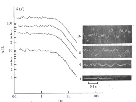
A typical time course of the current flowing through a single channel, undergoing the above stochastic process, is illustrated by the bottom trace of Fig. 1. This signal was obtained by simulating the random process described by (1) with a ~ fi and assigning arbitrary values to the two current levels, KJV and yV. Indeed, as discussed later, similar single channel current fluctuations are actually observed in BLM con- taining EIM. For such systems there would be hardly any need of pursuing further our theoretical analysis as done below. The verification that the statistical distributions of the lifetimes To and 7\ are simple exponentials provides in these cases a good test for the validity of the two-state model assumed above. Furthermore, the measurement of the two current levels and of the average lifetimes, To and Tx would yield all the channel parameters (7, K, a, and /?) which can possibly be obtained at this level of experimentation. In most cases, however, particularly when dealing with natural membranes, the observation of isolated single channel processes is impossible. The observed current is the sum of the contributions from a large number of channels which independently and simultaneously undergo random fluctuations.

It will be clear from what follows that the introduction of the covari- ance, <j>z{t), is then essential. For the single channel case, <j>i(t) is given by (see Appendix):

= {yVf ( s S y** Pi n«(f) - ( s A *)"], (7)

where the stochastic variable Y is defined as being equal to K in state (o) and equal to unity in state (1) {yo = K\ J i = !)• Substitution of equation (2) in (7) yields, after rearrangement

*, (8) where

0; I=yVY, (9)

(10)

/ being the mean current which flows through the channel, Y being the apparent probability of state (1) if one assumes K = o (only one state of non-zero conductance), and p being the variance of Y relative to the square of its mean. A regular markovian process, such as the one we have assumed so far, is ergodic. We shall then have, according to the Birkhoff theorem,

lim ~

T-*oo * J 0

where the time average on the left-hand side is the autocorrelation function of any actually observed current signal, I*(t), whose average value, /*, must also coincide with I. Furthermore, the power spectrum, Si(f)> of the signal I*(t), should be given, according to the Wiener- Khinchin theorem, by

Si(f) = 4 r

Jo cos znft 6t = 4/²pr/[i + W^l («) which is known as a Lorentzian spectrum. It is useful for later discus- sion also to derive from equations (2) the time evolution (relaxation) of the current expectation value, (/(*)) starting from state probabilities, and Pj⁰⁾, which are different from the stationary values, Po and Px:

From the simple expressions for niJ;(f) in (2), it is easy to verify that:

f > - F ) e - W , (14) - / ) e - ^ , (15) where

</(o)> = yVlKPiv+m = yV(Y(o)). (16)

Comparison of equation (15) with (8) illustrates, for the present particu- lar case, that the average relaxation toward equilibrium and the auto- correlation of the spontaneous fluctuations around equilibrium have the same time dependence.

We consider now the case of a membrane containing M independent but identical channels. At any instant of time the total current through the membrane will be the sum of the currents through each separate channel. It is a very simple result of elementary probability theory that the average value of the total current is just M times the average single channel current, given by equation (9). However, the most important result for fluctuation analysis is that also the autocorrelation function and the power spectrum of the total current are simply M times those of each individual channel, given by equations (8) and (12). It is then straightforward to write, for a membrane with M independent

two-state channels,

I = MvVY, (17)

fait) = M-U²p e-**, (18)

while the average current relaxation, (/(<)>, is still described by the same equation (15). It is important to stress that Y, p, and T in equations (17)- (19), are the same single channel parameters as are defined by (3), (9) and (10). Thus, equations (8) and (9) show that fluctuation analysis yields direct information about single channel parameters even when the number of channels is so large that elementary contributions to the total fluctuations are impossible to resolve. Equation (5) shows, on the other hand, that relaxation analysis yields comparatively poorer information, which concerns only the kinetics (T) of the elementary processes and not their size or their number.

Figure 1 illustrates how power spectrum analysis still leads to simple results despite the increasingly 'noisy' random signals which originate from an increased number of random elementary events. The insets show current fluctuations from a simulated membrane system contain- ing (from bottom to top) 1, 4, 8 or 16 two-state channels with a ~ /?.

In the latter case (top trace) single channel fluctuations are already practically inappreciable, and it is easy to realize that a further increase in the number of elementary events would render hopeless any direct analysis of the signals. The main part of Fig. 1 shows the power spectra

100 5 4 3 2 10

4 3

S(f)

0 1 s

0 1 10 100

Hz

Fig. i. Random current signals and related power spectral densities in a simulated membrane system containing an increasing number (indicated in the figure) of independent channels undergoing stochastic transitions between open and closed states. The single channel rate constants, a and /?

have approximately the same value ( ~ 20 s"¹). The amplitudes are in arbitrary units. Notice that the power spectra are merely proportional to each other according to the number of channels present.

obtained from long samples of the signals shown in the insets. All the spectra have exactly the same shape, corresponding to equation 19, with a low frequency amplitude which is merely proportional to the number of channels.

So far we have been considering current fluctuations for a constant voltage across the membrane. The properties of the fluctuations in the voltage across the membrane for a constant current are easily derived from the previous ones. Their power spectrum, Sv(f), must be related to 5/(/) through the complex membrane impedance, Z(f) (see e.g.

Wanke, De Felice & Conti, 1974):

Sy(f) = |^(/)| "/(y )> (20) Sv(f) is in general no longer a simple Lorentzian since the membrane impedance is rarely frequency independent, particularly in biological membranes or lipid bilayers which have a very large capacitance.

However, the knowledge of |Z(/)|² allows us in principle to unfold in a simple way the behaviour of Sj(f) from that of S_v(f). This is one of the contexts in which the spectral analysis offers great advantages with respect to the autocorrelation analysis. No simple relation as equation (20) exists between the voltage and current autocorrelation functions.

Fixed number of multistate channels

The case of M independent and identical channels, which can exist in more than two states, is conceptually identical to the previous one. If we indicate with yi the single channel conductance in state (i)(i= 1,2,..., r) the autocorrelation function of the current fluctuations around equili- brium, (j>i{t), and the relaxation of the average current towards equili- brium, <I(t)) — I, will be given by:

jkyt yk Pt nitk(t) )

-i = Mv\i iy_k^n_itk{t)-ip_i7i}, (22)

where P₄ is the stationary probability of state (1), Pj⁰⁾ is the initial prob- ability of state (i) in the relaxation process, and the transition probabilities ITi>fc(2) are the solutions of the system of linear differential equations:

^ - i ^ f l t t (23) with the initial conditions U_ik = 8_ik. The coefficients a_lk in equation (23) can be expressed in terms of the rate constants amn, where amn At represents the transition probability in time A* from state (m) to state (n):

«ifc = ^aki i^k * ']• (²4)

•m+k

Chen & Hill (1973) have derived formal expressions of <fii(t) and of its Fourier transform, Sj(f), for the most general multistate channel system described by equation (23). The formulas are, however, rather involved and we shall mention here only the most important qualitative results. Quite generally, the solution of (23) leads to an expression for (IIi(&(*) - Pk), which is a linear combination with constant coefficients, of ( r - i ) exponentially decaying functions with time constants solely determined by the rate constants amn, and independent of i and k.

Similar expressions consequently describe the time dependences of

<f>j(t) and (/(*))-/, both being linear superpositions of the Uiik(t) which decay to zero at infinite time. This is again a particular direct demon- stration of the equivalence between the time course of fluctuations and relaxations. Finally, the current noise power spectrum, Sz(f) is ex- pressed by a linear combination of (r— 1) simple Lorentzian spectra.

The multistate channel model which seems most relevant to the discussion of channel noise in nerve membranes can be treated easily without going through the formal solution of equation (23). Following Hill & Chen (1972a), we consider a generalization of the model which is implicitly assumed in the Hodgkin-Huxley (HH) description of voltage- clamp data (Hodgkin & Huxley, 1952). Each channel contains x in- dependent two-state subunits, each affecting the channel conductance through a multiplicative factor which depends on its state. For this case, the current through a single channel can be written as:

i = yvnji, (25)

where y is the maximum channel conductance and the stochastic variable Intakes the value of /q(< 1) or unity, depending on whether the subunit i is, respectively, in state (o) (yielding a lower conductance) or in state (1). The covariance and the average relaxation of the current, for a membrane containing M (independent) channels of this type, are then derived directly from simple properties of the product of independent variables:

= (y*W n

U=I

fi [1 + Pi e-^t/T'j - 1 j , (26)

i. (28)

<=i

The autocorrelation 4>i{i)y ^{a n}d the average relaxation, (/(*)>, in equa- tions (26) and (27) will in general contain 2^X— 1 different exponentials, and the power spectrum will be a linear combination of z^x — 1 Lorentz- ians. This is in agreement with the fact that, in general, the number of distinct states of our channel with * subunits is 2^X.

Three special cases of (26) are particularly relevant to the discussion of current noise in squid giant axons.

For four identical subunits, all characterized by the same rate constants, an and /?„, and for KX = KZ ... = o, equations (26) and (27) become:

W +/>ne-**«]«-1}, (29)

</(*)> = ill + ⁿl°k-? e-*/'«T; 1 = MyVn\ (30) where, according to equations (3), (9) and (10), in this particular case, Pn = fij*», n = <y> = an/ ( an+ / ? j , rn = i/(an+^n). The power spec- trum corresponding to (29) is given by:

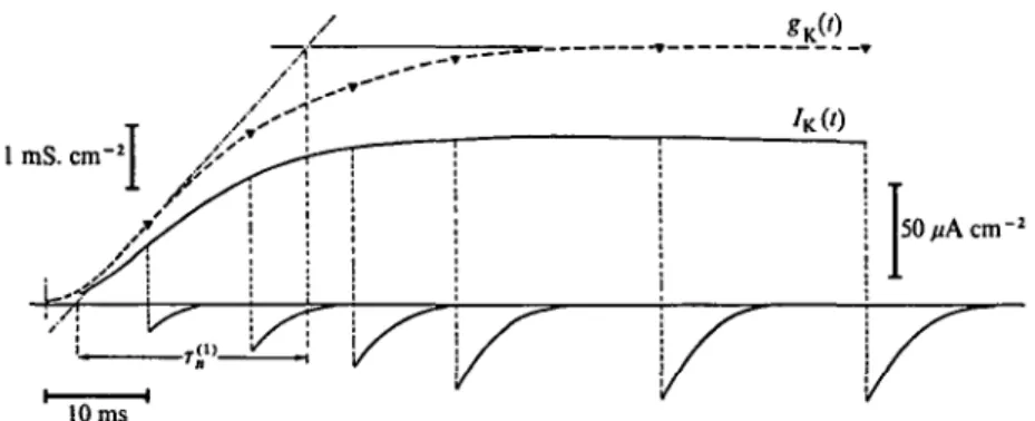
Si(f) = ± I^i^jpim + z-nrJiif}. (31) Equations (29) and (31) describe the current fluctuations due to the open-close kinetics of the potassium channels in nerve membranes, according to the simplest translation in stochastic terms of the HH equations, which are based on the description of relaxation (voltage- clamp) measurements according to equation (30).

A similar special case of equations (26) and (27) leads to the characterization of the noise from sodium channels, which according to the HH formulation are assumed to contain three identical subunits with rate constants am and ftm and a fourth subunit with rate constants cch and fih, /q being zero for all subunits. For this case:

-1}, (32)

rn

where pm = fijam, ph = fih/ah, and m, h, Tm and Th correspond to parameters used in the HH equations. The power spectrum corre- sponding to the autocorrelation function given by (32) can be approxi- mated for T_h > r_m (as in the case of the HH equations), as:

(34)

< = ]

Finally, for * identical subunits with KX = K2... = KX — K, equations (35) and (36) characterize the V case' of the generalized model of the potassium channels discussed by Hill & Chen (1972a) and Chen & Hill

<?>e-*/*>]«-1}, (35)

=/ [1 + < ^ M z I ^ e-t/rjr'j, I = M7V[YW]*. (36)

Fluctuations in channel number

The most general case of channel noise from independent channels also involves fluctuations in the number of existing channels. This further complication may for example be required in artificial lipid bilayers which may exchange channel-inducing substances with the bathing aqueous solutions. In addition to the rate constants for internal con- version it is then necessary to specify the channel formation rates in state (i), Ai( and the disappearance rate constants, fti0, fii0 At being the probability that a channel in state (i) disappears in time At. The auto- correlation function will again be of the form of a linear combination of exponentials. However, for r internal channel states we shall have in this case r (not r— 1) time constants,, all of which will depend both on the internal conversion rate constants, ai3- (i, j = 1,2,..., r) and on the disappearance rate constants fi_iQ (i = 1, 2, ..., r). The formation rates, Ai( will influence the average number of channels in the various states, and, therefore, the coefficients of the various exponentials in the auto- correlation function. A simple special case is obtained when, for any

s t a t e(0> R <* v „

fc*i,0

This condition implies that the lifetime of a channel in any state is long enough to allow equilibration among all possible internal channel states.

It can be shown that the current autocorrelation function for this special case is:

^{ ^ j } (37)

where M is the total average number of channels present at any time, independently of their internal state; (pi^t) and Ix are the covariance and the average value of the current which would flow through a single, permanent, channel; Pj is the equilibrium probability of state (i) for

such a permanent channel. The first contribution to ^(i) in equation (37) is identical to what is expected from M permanent channels.

The second contribution is due to the formation and disappearance of channels carrying an average current Iv For channels with only one

S t a t C :

<}>1{t) = MItt-l^lt = M-Wz-l^>t, (38) where Ix is the current through a single channel and /S"¹ is the average channel lifetime.

Channel noise modulating intrachannel noise

So far we have considered only the noise associated with fluctuations in the conductance or in the number of channels, and we have assumed that the current flowing through a channel in any fixed configuration is constant, free of what we may call intrachannel noise. Such assumption cannot be maintained in general, since thermal, shot and 1//noise are expected to be present anyway, even if the channels are stable single state pores. However, as shown below, our preceding simplified analysis is justified by the fact that, under certain conditions, channel noise and intrachannel noise are expected to be additive to one another.

Let us first consider the case of channels, with only one non-zero conductance value and assume that the current, /, through a single channel can be written as the product of two independent stochastic variables:

= y ^

where the fluctuations of J account for intrachannel noise and Y fluctuates between zero and unity. The assumption that the stochastic fluctuations of J are not influenced by the random switching of channel state is very reasonable for thermal or shot noise, which have very short correlation times. However, for 1//noise the independence of J and Y has no obvious justification other than that it predicts a 1//noise power proportional to the square of the average current, as observed experi- mentally in nerve membranes. From a simple property of the covariance of the product of independent variables, it follows from equation (39):

W <f>¥, (40)

For thermal noise or shot noise we expect 07 to decay to zero much faster than <j)Y so that ^>j (j)Y — <S>j 0 F ( ° ) > ^{a n}d :

(40

where the last equality derives from the fact that, in the present simple case, (Y = {o, 1}), <F>> = F.

For 1 If noise, we expect <fi_r to decay much faster than <pj so that

(42) It can be shown, with a slightly more involved argument, that equation (41) is more generally applicable to the case of an arbitrary number of channel conductance states, under the only assumption that the corre- lation times of Y are much longer than those of thermal or shot noise.

Rather than the independence of J and Y one should require in this case that the thermal or shot noise, during each channel state lifetime, have powers proportional respectively to the channel conductance or to the average current.

E X P E R I M E N T A L TECHNIQUES

The major technical problem in noise measurements is that of minimi- zing all possible sources of fluctuations that are not intrinsic to the system under study. Typical sources of unwanted disturbances are microphonics, electromagnetic pick-up, fluctuations in junctional emfs, (either metal-metal or metal-electrolyte), and amplifier noise. All these sources can be reduced through a careful design of the experimental apparatus. Alternatively, or in addition, ways of subtracting extraneous noise from the noise under study can often be found.

In membrane studies, electrode noise is of particular concern, since it is not easily removed a posteriori. Pt-Pt black electrodes with a low impedance down to low frequencies are particularly recommended, as an alternative to Ag-AgCl (Wanke et al. 1974).

Amplifier noise deserves special discussion. Design techniques exist for assemblage of available components for lowest noise performance (see e.g. Motchenbauer & Fitchen, 1973), but the lowest attainable levels of amplifier noise depend ultimately on the quality of the commercially available solid-state devices. The input stage is usually the most critical part of the set-up, and selected junction field effect tran- sistors (JFET) should be employed for it. Apart from the above general comments, the problem of amplifier noise presents different aspects for different membrane preparations, and depending on whether current noise or voltage noise is measured. These have been discussed

10-^{1 3} V²/Hz

© 10-^{2 0} A²/Hz

10⁷ n²

no. 19 9-5 °C .4=0-36 cm²"

11111*

10 100 1000

Hz

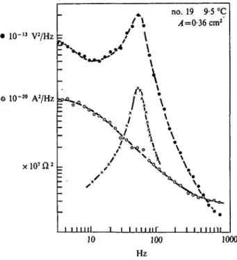
Fig. 2. Current noise power spectrum, O, voltage noise power spectrum, 0 , and the square modulus of the impedance, x , in a large area (0-36 cm⁸) of squid axon membrane at resting potential in normal physiological condi- tions. Temperature: 9 °C. (From Wanke et al. 1974.)

in detail by various authors, for example Derksen (1965) and Siebenga, Meyer & Verveen (1973) for frog node preparations; Poussart (1971) and Fishman (1973, 1975) for artificial node preparations in giant axons; Wanke et al. (1974), De Felice, Wanke & Conti (1975), and Conti, De Felice & Wanke (1975) for large areas of squid axon membrane.

The difference between voltage-noise and current-noise measurements is worth stressing here. As already mentioned, the two measurements yield in principle the same information provided the membrane im- pedance locus is known (equation (20)), but Sj(f) can be directly related to channel noise, without requiring supplementary impedance studies.

Sj{f) and Sv(f) are expected to be quite different particularly in well isolated areas of nerve membrane, whose impedance varies strongly in the range of frequencies where channel noise is studied (Wanke et al.

1974). This is illustrated in Fig. 2, showing plots of experimental mea- surementsof Sv(f), Sz(f) and |Z(/)|², from the same preparation of squid

giant axon. The contrasting result reported by Fishman (1973), that current noise and voltage noise spectra from very small patches of squid axon membrane are practically identical, must be due to the large shunt conductance in parallel with the artificial node (Fishman, 1975), creating a poor isolation of the node (see also Pooler & Oxford, 1972).

Invasion of currents from lateral regions bordering the gap might seriously impair in this preparation the possibility of actually clamping either the current or the voltage in the central area under study.

The advantage of obtaining more direct information from current noise is obtained at the expense of simplicity of the measuring setup.

The measurements must be performed under voltage-clamp conditions using special feedback circuits whose specifications have been discussed in detail by Poussart (1971, 1973)-

When some freedom in selecting the membrane area under study is allowed, the problem of optimizing such area for best membrane noise detection is of some importance. It can be shown quite generally (see e.g. De Felice et al. 1975) that the maximum ratio between membrane noise and amplifier noise is obtained when: \Z\² = e²/*². Here Zis the membrane impedance, and e^ and i\ are the voltage and current spectral densities of the amplifier input noise. The above relationship cannot in general be satisfied at all frequencies, but it leads anyhow to an esti- mate of the optimal range of membrane impedances and, therefore, of membrane areas. It should be stressed, however, that such optimization is not always critical, while other considerations may actually make it preferable to depart considerably from it. For example, typical figures for the input noise of commercially available electronic devices

(e² ~ io-¹⁶ V² s; i\ ~ io-²⁸ A² s)

lead to optimal membrane impendances of the order of 1 MQ. For the squid axon membrane (\Z\ ~ 1 Kfi cm² at low frequencies, and

\Z\ ~ 160 Q. cm² at 1 KHz), this corresponds to an optimal area of io"³ cm² or less, and such an estimate seems to have been the leading motivation for the use of artificial nodes (Fishman, 1975). However, recent experiments (Wanke et al. 1974; De Felice et al. 1975; Conti et al. 1975) have shown that the requirement of optimal area can be freely disobeyed without seriously impairing good membrane noise detection. Working with much larger membrane areas (~ 0 3 cm²) leads to great advantages, such as an easier nerve preparation to set up, with better control of its physiological and isolation properties.

30 QRB 8

The analysis of the random noise signals may constitute a major part of noise experiments. However, a discussion of the problems in- volved in signal processing (e.g. anti-aliasing filtering, sampling, time windows, etc.) is beyond the scope of the present review and can be found elsewhere (e.g. Rabiner & Rader, 1972). Furthermore, present day noise analysis is often greatly simplified by the availability of special purpose machines, such as correlators or power spectrum analysers, which can process directly on-line the analogue random signal, having all the necessary processing steps built in. Alternatively, analogue data stored on magnetic tape can easily be processed with digital com- puters using standard available software (e.g. the Fourier Analyzer System HP 5451A). A general theoretical result which is worth keeping in mind is that the accuracy of noise data increases as the square root of the duration, T, of the analysed noise sample. Thus, the ratio between the standard deviation and the average value of the measured noise power in the frequency interval, A/, is approximately equal to (TA/)-¹^ (Rice, 1944).

Whether to analyse noise signals in terms of autocorrelation functions or power spectra may be in many cases a matter of convenience or taste.

However, in studies of nerve membranes, power spectra are largely preferred, since they allow an easy separation of channel noise from 1//noise, and even when correlation analysis is used, the data are finally converted into power spectra through a Fourier transformation (Sie- benga et al. 1973; Siebenga, De Goede & Verveen, 1974). On the other hand, the noise from lipid bilayers containing gramicidin A does not show a significant 1// component, and has preferably been analysed in terms of its autocorrelation function (Neher & Zingsheim, 1974; Zing- sheim & Neher, 1974; Kolb et al. 1975).

N O I S E FROM NERVE MEMBRANES Early studies (1 If noise and burst noise)

The first studies of membrane noise, performed on the node of Ranvier of isolated frog sciatic nerve fibres, were published in 1965 (Derksen, 1965; Verveen & Derksen, 1965). In addition to thermal noise, the membrane voltage was found to contain a large excess noise of the 1//

type in the range of frequencies from o-i to 10 000 Hz. Compelling evidence suggested that the 1// noise was mainly associated with the

passive movement of potassium ions, and this result was confirmed by later experiments on the same preparation (Derksen & Verveen, 1966;

Verveen & Derksen, 1968; Siebenga & Verveen, 1970) and also on giant axons of lobsters (Poussart, 1971). A detailed discussion of 1//noise in nerve membranes is given by Verveen & De Felice (1974). We believe that quantitative experimental studies of 1//noise, together with a better theoretical understanding of its origin, will eventually yield some information about ion-ion and ion-channel interactions in the ionic channels of nerve membranes, but clear results in this direction are still missing.

The measurements of small voltage fluctuations in frog nodes showed also the presence of another type of excess noise which became generally evident only for large hyperpolarizations, in the form of irregularly occurring miniature depolarizing potentials (Derksen, 1965;

Verveen & Derksen, 1968, 1969). This was termed by the above authors ' burst noise'. It was found to be independent of the extracellular concentration of potassium and of resting potential, while substitution of sucrose for extracellular NaCl shifted its appearance toward higher hyperpolarizations. From these observations it was speculated that burst noise could be associated to the passive movement of sodium ions, or even with the random opening of sodium channels (Verveen &

Derksen, 1969). The latter interpretation seems untenable since burst noise increases, while the probability of opening of sodium channels decreases, with increased hyperpolarization. The absence of any effect of the sodium channel blocking drug, tetrodotoxin (TTX), upon burst noise (Siebenga et al. 1974), leads to the same conclusion (Verveen

& De Felice, 1974). The association of burst noise with sodium ion flow was suggested mainly by the NaCl versus sucrose substitution experiment. However, it is known (Conti, Fioravanti & Wanke, 1973) that lowering the ionic strength of the extracellular solution increases drastically the membrane potential at which (macroscopic) membrane dielectric breakdown occurs. Thus, the results of such experiments are also consistent with the hypothesis that the bursts are transient localized dielectric breakdowns (Del Castillo & Katz, 1954). Such an hypothesis is further supported by the observation of very similar phenomena in simple lipid bilayers (Yafuso, Kennedy & Freeman, 1974).

30-2

Evidence for channel noise

In more recent years, experiments on depolarized nodes of Ranvier have revealed the presence of other additional voltage noise components which could be described fairly well as simple Lorentzian noise added on top of i// noise (Siebenga & Verveen, 1971, 1972; Siebenga et al.

1973, 1974). The order of magnitude, and the temperature dependence of the Lorentzian cut-off frequency were found to be in qualitative agreement with the expected behaviour of the noise due to fluctuations in the conductance state of the ionic channels governing the late (potas- sium) voltage-clamp current. The most compelling evidence for the identification with potassium channel noise was the sensitivity to the addition of tetraethylammonium ions (TEA) (Siebenga et al. 1974).

A quantitative account of the observed Lorentzians in terms of the HH description of relaxation (voltage-clamp) experiments, was not given.

As discussed below, this requires the direct comparison of voltage-clamp and noise data from the same preparation, and according to the same microscopic model of channel kinetics. Thus, the potassium channel density of 1000/im~², estimated by Siebenga et al. (1973) (according to a model implying only two channel states of equal probability) although indicative, might be very inaccurate. Using a more general model, in which each channel is assumed to have only one possible non- zero conductance value (but an arbitrary number of states), Begenisich

& Stevens (1975) have obtained an estimate of the single potassium channel conductance, from their measurements on frog nodes, of 4 x i o ~^{1 2}S . This value is about six times smaller than the average estimate of Siebenga et al. (1973).

Very recently it has also been reported that the Lorentzian noise component expected to be associated with the h process in sodium channels (the first component in equation (34)) can be observed in depolarized frog nodes after blocking the potassium current with intra- cellular caesium ions and TEA (Van den Berg, 1975). Although de- tailed data have not been published yet, the results seem to be in good agreement with the simple HH model and to lead to a correct estimate (2-4 x io~¹² S) of the single sodium channel conductance (see later).

Observations of channel noise have been reported also for artificial nodes (Fishman, 1973, 1975) and for large voltage-clamped areas (Wanke et al. 1974; De Felice et al. 1975; Conti et al. 1975) of the squid

giant axon. The results of the latter experiments will be discussed in detail in the next section. As mentioned in experimental techniques (pp. 467-8), the sugar gap artificial node preparation is subject to criti- cism, there being doubts about the unequivocal correlation between the observed 'humps' in the noise spectra, and potassium channel noise (Wanke et al. 1974). It seems that, with such a technique, what one really measures are the voltage fluctuations across the shunt resistance in the gap regions, due to current fluctuations both in the central (clamped) area and in the lateral (uncontrolled) regions. Thus, while Fishman's obser- vations may indicate qualitatively the presence of potassium channel noise in squid axons, it seems clear that the results are very difficult to interpret quantitatively.

Channel noise in voltage-clamped squid giant axons

Noise measurements from long (~ 20 mm) segments of squid giant axons, well isolated from lateral regions by air-gaps, and kept under good space- and voltage-clamp conditions, can be performed using techniques described elsewhere (Wanke et al. 1974; De Felice et al.

1975; Conti et al. 1975). In addition to the good control of its physiologi- cal and isolation properties, this preparation offers major advantages such as the possibility of simultaneous noise and average current measurements, together with an independent continuous monitoring of the absolute membrane potential. Furthermore, measurements of large voltage-clamp currents under exactly the same conditions and possibly in the same axon, allow a direct comparison between macroscopic relaxation and noise data, needed for quantitative analysis of the results.

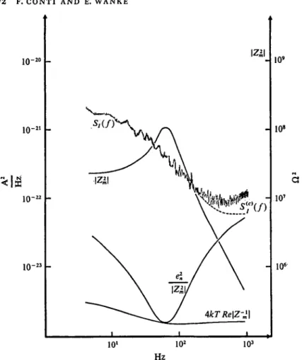
A typical current noise power spectrum, S^f), from an axon voltage clamped near its resting potential at a temperature of 9 °C is shown in Fig. 3. The figure contains also a plot of the membrane impedance modu- lus squared, \Z_m\², measured from small sine wave analysis (Conti, 1970), from which the amplifier's noise contribution, e|/|Z_m|², and the theoretical thermal noise, ^kTRe(Zm)~^x, could be evaluated. It is seen that, apart from a small correction for frequencies above 200 Hz most of the measured noise can be attributed to excess (non-thermal) mem- brane noise shown in the figure as 5/^c)(/). Fitting the power spectrum of Fig. 3 with a straight line would lead to a slope very close to — 1 showing the presence of a major 1//noise component. However, signifi- cant departures from such a straight line are also apparent and were

10"

10-

10"

10"

10'

10⁸

io⁷

io⁶

io² io³

Hz

Fig. 3. Current noise spectral density, S/(/), and the square amplitude of the impedance, \Zm\^s, in a squid axon membrane, plotted together with the expected Nyquist noise, ^kTReZ^¹, and amplifier noise, ejJ/IZml²- The dashed line, >S/^c)(/), gives the membrane current noise spectrum corrected for the latter contribution. Temperature: 9 °C. Membrane area 0-32 cm², Vm = — 56 mV. (From Conti et al. 1975.)

attributed to channel noise modulation of intrachannel, mainly 1//, noise (Conti et al. 1975).

According to the HH analysis of voltage-clamp experiments (Hodgkin

& Huxley, 1952) and following the theory previously discussed, the power spectrum, Sj^(c\f) should be dissected into the sum of three components with distinct spectral characteristics. 1//noise, as a general characteristic of passive ionic fluxes (De Felice & Firth, 1970; Hooge

& Gaal, 1970; De Felice & Michalides. 1972; Michalides, Wallaart &

De Felice, 1973) is expected to affect the currents flowing through the

10-

10-

10-

, IZJ²

10¹ 10² 10³

Hz

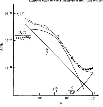
Fig. 4. Current noise spectral density Si(f) from a squid axon treated with 20 nM TTX at V_m = — 53 mV. The dashed line is the sum of a Lorentzian, a 1// component and the amplifier noise e%/\Zm\^a. The three separate com- ponents an: drawn as continuous lines. Temperature: 9 ^CC. Membrane area 0-28 cm². (From Conti et al. 1975.)

leakage pathway and through the potassium or sodium selective channels.

The random opening and closing of these channels is further expected to produce current fluctuations with power spectra which are sums of a small number of Lorentzians (see equations (31) and (34)). Distinct spectral characteristics of the sodium versus potassium channel noise are expected on the basis of the different relaxation times which characterize the kinetics of the two types of channels (see e.g. Fig. 3.32 of Cole, 1968).

K channel noise. The actual extraction of potassium channel noise, SK(f), from <Sj^(c'(/) can be most easily performed by eliminating sodium currents with TTX (Narahashi, Moore & Scott, 1964) and approxima- ting the sum of Lorentzians in equation (31) with a simple Lorentzian.

In the range of membrane voltages explored by Conti et al. (1975), this approximation seems fairly justified according to the actual values for

10"^{2 0}

10"²

\

5;( / ) Axon 33 TTX

10¹ 10² 10³

Hz

Fig. 5. Current noise spectral density for Vm = — 41 mV, from an axon injected intracellularly with 70 mM-TEAchloride, compared with the spectrum at the same Vm from an axon treated with 20 nM TTX. The two axons had approximately the same area (031 cm²) and the two spectra were obtained at the same temperature, 9 °C. The continuous lines show the two components (i//+Lorentzian) whose addition approximates each spectrum. The arrows indicate the half power points of the Lorentzian com- ponents. (From Conti et al. 1975.)

the potassium channel parameters extracted from voltage-clamp data.

SK(f) can then be extracted from TTX treated axons by expressing the total noise (apart from amplifier noise correction) as the sum of a 1//

component and a simple Lorentzian. This procedure is illustrated in Fig. 4. It is seen that the fitting of the measured spectrum with the sum of the three solid lines, representing 1//, Lorentzian and amplifier noise, is quite good down from 5 Hz up to 500 Hz. The slight discrepancy in the range from 500 Hz to 1 KHz could be due to a slightly wrong

estimate of the amplifier noise, which becomes predominant at such frequencies. Should it have any real significance it would constitute any- how a minor feature of the overall spectrum.

An independent check that SK(f), extracted with the above procedure is associated with K channel noise is obtained by studying the noise from axons containing intracellular concentrations of TEA sufficient to block the potassium currents completely (Tasaki & Hagiwara, 1957; Arm- strong & Binstock, 1965). Fig. 5 shows the current noise power spectrum from an axon treated with 70 mM-TEA and held at a membrane potential, Vm, of —41 mV, as compared with the spectrum from a TTX-treated axon at the same V_m and temperature (9 °C). The whole low-frequency region of the TTX spectrum is seen to be strongly depleted by TEA.

On the other hand, the TEA spectrum becomes larger than that of TTX at high frequencies, a feature which is expected from the presence of the sodium channel noise, discussed below.

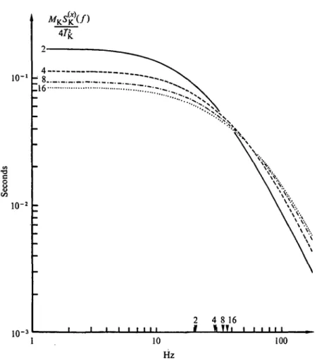
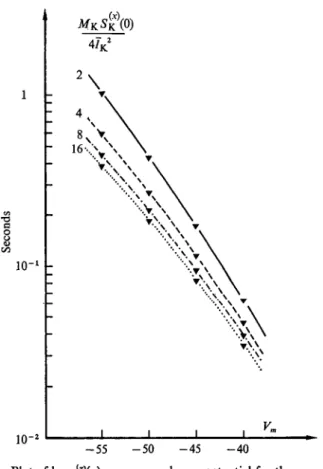
At the level of approximation implicit in the extraction procedure of Fig. 4, SK(f) is fully characterized by its low frequency limit, SK(o), and by the cut-off frequency, /⁽^p, at which SK(f⁽^) = SK(o)J2. In agreement with the theoretical expectation of the simple model leading to equation (31), the experimental results of Conti et al. (1975) showed a temperature dependence of SK{6) or /⁽jp, which was very close to that of r_n (Q₁₀ ~ 3) or i/r_n. The slight dependence of /⁽f' on membrane potential and the range of its experimental values also agreed with the simple HH kinetic model. Furthermore, the strong voltage dependence of SK(o) could be fitted fairly well according to (31), using the HH voltage-clamp parameters appropriately extracted from the same giant axon preparation. The fitting obtained by Conti et al. (1975) is shown by the dots and the solid line in Fig. 6, where similar data for the sodium channel noise, to be discussed below, are also reported. Since, for any model of independent channels, the absolute value of the current noise power for a fixed average current is simply inversely proportional to the number of channels, such fitting leads to an estimate of the density of potassium channels, MK, which, according to the simplest HH model, was found to be of the order of 60 fiver². This estimate was little affected by the particular model assumed for the potassium inactiva- tion process (Ehrenstein & Gilbert, 1966), which is anyhow small in the range of Vm applicable to the data of Fig. 6. A discussion of how critical, for the estimate of M_K, the assumption of the simple HH channel kinetics is, and of the relevance of the above results for restricting the