with Satellite Observations

with Satellite Observations

Inaugural-Dissertation zur

Erlangung des Doktorgrades

der Mathematisch-Naturwissenschaftlichen Fakultät der Universität zu Köln

vorgelegt von Sonja Reitter aus Rotenburg/Wümme

Köln 2013

Tag der mündlichen Prüfung: 24. Oktober 2013

Ice clouds are an important part of the Earth’s atmospheric water cycle and have a large im- pact on the global radiation budget. Yet ice clouds are still poorly understood and their cor- rect representation remains a major challenge for state-of-the-art atmospheric models. Also, the evaluation of the models’ performance with respect to ice clouds is not straightforward;

remote sensing instruments, for example, measure other quantities than the models predict.

Therefore, two basic evaluation approaches exist: observation-to-model (commonly termed retrieval) and model-to-observation (commonly termed forward operator). Both approaches introduce errors into the comparison of models and observations because of the necessary intrinsic assumptions. The common practice in model evaluation of choosing either the one or the other of these approaches might give an incomplete picture.

The present study evaluates the ice microphysics of two numerical weather prediction

(NWP) models currently operational at the German weather service (Deutscher Wetter-

dienst, DWD): the global model GME and the regional model COSMO-DE (an application

of the Consortium for Small-scale Modelling, COSMO). In doing so, this study contributes

significantly to ongoing model development at DWD. Both case studies and long-term eval-

uations are carried out. Cloud Satellite (CloudSat) Cloud Profiling Radar (CPR) observa-

tions are heavily relied on; the CPR is the first and — up to date — only cloud radar in

space and is able to vertically resolve even optically thick clouds. This study focuses on

one specific question raised for each of the respective models and while doing so applies

both approaches; the standard CloudSat radar reflectivity factor–ice water content (IWC)

retrieval for the observation-to-model approach and the forward operator QuickBeam for

the model-to-observation approach. This enables for one, to profit from the full informa-

tional content, and for the other, to compare both approaches directly to each other and

evaluate them.

For the global model GME, two precipitation schemes, a diagnostic and a prognostic one, are compared and evaluated. The focus is on the question whether the new prognostic scheme is capable of capturing ice clouds more realistically than the old diagnostic scheme.

The prognostic scheme is shown to exhibit improved performance in comparison to the di- agnostic scheme in terms of IWC magnitude. In both models snow is found to dominate over cloud ice in total IWC, emphasizing the need for including snow in the model’s radi- ation budget in the future. Furthermore, one reason for the remaining difference between the prognostic scheme and the observations — the unrealistic fall speed of snow — is iden- tified. As a consequence, the new prognostic scheme with an adapted parameterization for snow fall speed was successfully introduced into operational service at DWD.

In the regional NWP model COSMO-DE, a long-known bias between brightness tempera- tures simulated from COSMO-DE forecasts and those observed by Meteosat Second Gen- eration (MSG) Spinning Enhanced Visible and Infrared Imager (SEVIRI) is investigated.

The pivotal question is whether a novel two-moment cloud ice scheme exhibits improved performance with respect to this bias and, if that is so, why. It is shown that the novel two- moment cloud ice scheme does indeed reduce this bias and can therefore be considered an improvement in comparison to two standard schemes, the two-category ice scheme and the currently operational three-category ice scheme. The improvement in simulated brightness temperatures is due to a vertical redistribution of cloud ice to lower model levels. Further- more, sensitivity studies identify two of the four changes introduced, which are responsible for most of the improved performance: the change to a different heterogeneous nucleation scheme and the inclusion of cloud ice sedimentation. Enhanced vertical level number and modifications in aerosol number concentrations reveal comparatively little effect. As a con- sequence, cloud ice sedimention will be included per se in DWD’s future NWP model, the Icosahedral non-hydrostatic (ICON) model, currently still under development.

Concerning the two evaluation approaches conducted, the present study finds the general

features in the two evaluations to be captured by both approaches. Some details are captured

merely by the one or the other approach, in which case both approaches together give the

more complete picture. However, the model-to-observation approach appears to be easier

to interpret; its uncertainties are easier to assess than those of the observation-to-model

approach and it ensures a better control over the comparison.

Eiswolken sind ein wichtiger Bestandteil des atmosphärischen Wasserkreislaufs der Erde und haben einen großen Einfluss auf den globalen Strahlungshaushalt. Dennoch sind Eis- wolken bisher nicht vollständig verstanden. Dies führt unter anderem dazu, dass ihre kor- rekte Darstellung in aktuellen atmosphärischen Modellen weiterhin eine große Heraus- forderung darstellt. Die Evaluierung dieser Modelle hinsichtlich ihrer Fähigkeit Eiswolken vorherzusagen ist nicht trivial: Beobachtungsdaten von Eiswolken, zum Beispiel von Fern- erkundungsinstrumenten, liefern andere Größen als die, die Modelle vorhersagen. Aus diesem Grund existieren zwei wesentliche Evaluierungsansätze: Beobachtung-zu-Modell (üblicherweise als Retrieval bezeichnet) und Modell-zu-Beobachtung (üblicherweise als Vorwärtsoperator bezeichnet). In beiden Ansätzen müssen Annahmen gemacht werden, die zu Unsicherheiten im Evaluierungsprozess führen. Zumeist wird nur einer der beiden An- sätze verfolgt, was zu einem unvollständigen Bild führen kann.

In der vorliegenden Arbeit wird die Eismikrophysik zweier numerischer Wettervorhersage-

modelle (NWP-Modelle) evaluiert, die beim Deutschen Wetterdienst (DWD) aktuell ope-

rationell im Einsatz sind: das globale Modell GME und das regionale Modell COSMO-

DE (einer Anwendung des Consortium for Small-scale Modelling, COSMO). Damit liefert

diese Arbeit einen wichtigen Beitrag zur fortlaufenden Modellentwicklung beim DWD. Es

werden sowohl Fallstudien als auch Langzeitevaluierungen durchgeführt. Dazu werden die

Beobachtungen des Cloud Satellite (CloudSat) Cloud Profiling Radar (CPR), des ersten und

bisher einzigen Wolkenradars im All, extensiv genutzt. Der Vorteil des CPR ist, dass es selb-

st optisch dicke Wolken vertikal auflösen kann. Die Studie konzentriert sich auf jeweils eine

spezifische Frage pro Modell und verfolgt bei der Evaluierung von GME und COSMO-DE

beide möglichen Ansätze: das Standard-Eiswassergehalt (IWC)-Retrieval aus den Cloud-

Sat Radarreflektivitäten für den Beobachtung-zu-Modell-Ansatz und den Vorwärtsoperator

QuickBeam für den Modell-zu-Beobachtung-Ansatz. Dies ermöglicht es zum einen den gesamten Informationsgehalt auszuschöpfen und zum anderen die beiden Ansätze direkt miteinander zu vergleichen und zu bewerten.

Für das globale NWP-Modell GME werden zwei Niederschlagsschemata, ein diagnosti- sches und ein prognostisches, miteinander verglichen und bewertet. Zentrale Frage ist, ob das neue prognostische Niederschlagsschema in der Lage ist, Eiswolken realistischer darzu- stellen, als das alte diagnostische Niederschlagsschema. Es wird gezeigt, dass das progno- stische Schema eine realistischere Größenordnung des IWC wiedergibt, als das diagnosti- sche Schema. In beiden Modellen dominiert Schnee gegenüber Wolkeneis im Gesamt-IWC.

Dies unterstreicht die Notwendigkeit, Schnee im Strahlungsschema des Modells zukünftig mit zu berücksichtigen. Desweiteren wird ein Grund für den verbleibenden Unterschied zwischen dem prognostischen Schema und den Beobachtungen, nämlich die unrealistis- che Fallgeschwindigkeit von Schnee, identifiziert. Infolgedessen wurden das neue progno- stische Schema mit einer angepassten Fallgeschwindigkeit von Schnee erfolgreich in den operationellen Betrieb des DWD eingeführt.

Im regionalen NWP-Modell COSMO-DE wird ein bereits lang bekannter Bias zwischen den aus COSMO-DE Vorhersagen simulierten Helligkeitstemperaturen und den von Meteosat Second Generation (MSG) Spinning Enhanced Visible and Infrared Imager (SEVIRI) beobachteten untersucht. Zentrale Fragestellung ist, ob das neue Zwei-Momenten- Wolkeneisschema bezüglich dieses Bias besser abschneidet, und wenn ja, warum. Es zeigt sich, dass das neue Zwei-Momenten-Wolkeneisschema diesen Bias tatsächlich reduziert und somit eine Verbesserung zu zwei Standard-Eisschemata, dem Zwei-Kategorie- Eisschema und dem momentan operationellen Drei-Kategorie-Eisschema, darstellt. Die Verbesserung in den simulierten Helligkeitstemperaturen beruht auf einer vertikalen Um- verteilung des Wolkeneises in tiefer liegende Modellschichten. Sensitivitätsstudien zeigen zudem, dass zwei der insgesamt vier eingeführten Änderungen für einen Großteil der ver- besserten Darstellung verantwortlich sind: der Wechsel zu einem anderen heterogenen Eis- nukleationsschema und das Einführen der Sedimentation von Wolkeneis. Eine erhöhte ver- tikale Schichtzahl und Änderungen der Aerosolanzahldichten haben einen vergleichsweise geringen Effekt. Infolgedessen wird Wolkeneissedimentation im zukünftigen NWP-Modell des DWD, dem Icosahedral non-hydrostatic (ICON) Modell, standardmäßig implementiert.

Bezüglich der zwei verfolgten Ansätze zeigt die vorliegende Arbeit, dass die Grundaus-

sagen der Evaluierungen von beiden Ansätzen wiedergegeben werden. Manche Details

sind allerdings nur mit dem einen oder dem anderen Ansatz identifizierbar. Beide An-

sätze zusammen liefern demzufolge das umfassendste Bild. Der Modell-zu-Beobachtung-

Ansatz scheint jedoch in der Interpretation eingängiger zu sein: die hier auftretenden Un-

sicherheiten sind leichter abzuschätzen als beim Beobachtung-zu-Modell-Ansatz und er-

möglichen eine bessere Kontrolle über den Vergleich.

Abstract i

Zusammenfassung iii

1 Introduction 1

1.1 Motivation . . . . 1

1.2 Objectives . . . . 5

1.3 Overview . . . . 6

2 Cloud microphysics 9 2.1 Cloud microphysics in nature . . . . 9

2.2 Cloud microphysics in NWP models . . . . 15

3 Model data 21 3.1 GME . . . . 21

3.1.1 General aspects . . . . 22

3.1.2 Cloud microphysics: Two-category ice scheme . . . . 23

3.1.3 GMEdiag . . . . 26

3.1.4 GMEprog . . . . 28

3.2 COSMO-DE . . . . 30

3.2.1 General aspects . . . . 30

3.2.2 Cloud microphysics: Three-category ice scheme . . . . 32

3.2.3 COSMO-DE9009 (three-category ice scheme) . . . . 34

3.2.4 COSMO-DE8819 (two-category ice scheme) . . . . 35

3.2.5 COSMO-DE8822 (two-moment cloud ice scheme) . . . . 35

4 Satellite observations 41

4.1 CloudSat CPR . . . . 43

4.2 CALIPSO CALIOP . . . . 46

4.3 MSG SEVIRI . . . . 48

5 Retrievals and forward operators 51 5.1 CloudSat IWC retrieval . . . . 51

5.2 QuickBeam . . . . 57

5.3 RTTOV and SynSat . . . . 63

6 Evaluation of GME 67 6.1 Posing the question . . . . 67

6.2 Matching GME and CloudSat CPR – Part I . . . . 69

6.3 Case study . . . . 69

6.4 Statistical approach . . . . 80

6.4.1 Matching GME and CloudSat CPR - Part II . . . . 80

6.4.2 Results . . . . 81

6.5 Summary and conclusions . . . . 87

7 Evaluation of COSMO-DE 89 7.1 Posing the question . . . . 89

7.2 Statistical approach . . . . 91

7.2.1 Matching COSMO-DE and satellite data - Part I . . . . 91

7.2.2 Results . . . . 92

7.3 Case study . . . . 95

7.3.1 Matching COSMO-DE and satellite data - Part II . . . . 96

7.3.2 Results . . . . 96

7.3.3 Sensitivity experiments . . . 104

7.4 Summary and conclusions . . . 120

8 General summary, conclusions, and outlook 123

References 127

Appendices I

Danksagung IX

Erklärung XI

1.1 Motivation

Ice clouds have a large impact on the Earth’s climate system due to their role in the atmo- spheric water cycle and their effects on the global radiation budget. Of the various parts in the complex chain of processes of the atmospheric water cycle, ice clouds are one of the least well-understood parts and therefore add to the uncertainty in precipitation forecast.

Concerning their radiative impact, ice clouds contribute to the radiation budget through shortwave albedo and longwave greenhouse effects (Chen et al., 2011). The Intergovern- mental Panel on Climate Change (IPCC) states in its 4th assessment report that clouds in general and their radiative effect in particular are not yet well understood (IPCC, 2007).

The annual mean ice water path (IWP)

of the global climate models (GCMs) contributing to this report varies by two orders of magnitude (Waliser et al., 2009; cf. Fig. 1.1). Waliser et al. (2011) investigate the impact of frozen phase precipitation on the global radiation balance and find its neglection to lead to an overestimation of up to 10 % of integrated column cooling. Li et al. (2013) attribute the persistence of a systematic bias in top of at- mosphere radiative fluxes in the Coupled Model Intercomparison Project Phase 3 (CMIP3) and Phase 5 (CMIP5) simulations partly to the neglection of the radiative effects of precip- itating frozen phase. This illustrates the fact that a good description of ice clouds is still a major challenge for both GCMs and numerical weather prediction (NWP) models. Fur- thermore, it emphasizes the importance of including not only realistic ice clouds but also frozen phase precipitation in the radiation schemes of atmospheric models in order to ob- tain a realistic radiation balance. However, the consideration of frozen phase precipitation in radiation schemes is currently not standard in NWP models. Before this becomes reason-

*

Throughout the present study the term ice water path (IWP) refers to the sum of all columnar integrated

atmospheric frozen phase water, regardless of its habit.

Figure 1.1:

Annual mean values of IWP in g m

from the 1970-1994 period of the twentieth century GCM simulations contributing to the IPCC 4th Assessment Report (20c3m scenario). Note that the colour scale is not linear. From

able, the representation of ice cloud microphysics in models needs to be improved. Also, due to increased available computational power, the general trend in model development is heading towards increased model resolution on the one hand and attempts to describe frozen phase in more detail on the other hand. Especially the latter is noted by Avramov and Harrington (2010) who investigate the influence of different particle habits on model results. With all this, the importance of good ice cloud microphysical schemes increases.

At the German weather service (Deutscher Wetterdienst, DWD), efforts are in progress to

develop an efficient cloud microphysical scheme which is both physically consistent and

computationally efficient. Before entering operational forecast service, new schemes are

first corrected for potential numerical issues and code errors. Subsequently, they are inter-

nally verified at DWD to ensure that their performance with regard to certain standardized

skill scores (e. g. for surface precipitation) is better than that of the former scheme. The

former scheme could potentially produce better results even though it might be physically

less reasonable, because it is already tuned towards best results. Therefore, new schemes

are run in parallel routine for some time and only become operational once they actually perform better than the former scheme. In addition to this internal routine verification, fur- ther evaluation outside DWD is desirable, since it ensures the comparison with more special observational data. At operational weather forecast centers, these data might either not be available, or the time for more detailed evaluation might be lacking. The comparison of model and observation data is a challenging task. Instruments, retrievals, and forward oper- ators can exhibit strong sensitivities to factors such as particle size, and the microphysical schemes of the models vary greatly in configuration and complexity.

Both the development and the evaluation of such a cloud microphysical scheme require suitable observational data. Small ice crystals remain one of the most difficult objects to be observed. In situ measurements with aircrafts are affected by crystal shattering on probe tip or inlet shroud and overestimate small ice crystal concentrations by a factor of two (Mc- Farquhar et al., 2007). More recent campaigns try to reduce these errors with improved measurement techniques (Zhang et al., 2013). Remote sensing in general has to cope with instrument sensitivity limits. Ground-based remote sensing additionally suffers from atten- uation losses when having to penetrate thick clouds. This leaves space-based or airborne remote sensing as the best contemporary measurement technique for obtaining information from cloud top in the atmosphere. The Cloud Satellite (CloudSat) Cloud Profiling Radar (CPR; Stephens et al., 2002) is the first and — up to date — only cloud radar in space. It offers the unique opportunity to vertically resolve even thick ice clouds from space — in contrast to the numerous passive satellite-based sensors as, for example, Meteosat Second Generation (MSG) Spinning Enhanced Visible and Infrared Imager (SEVIRI). Due to its high resolution and the near-global coverage (compared to ground-based radars) the Cloud- Sat CPR is predestined for the evaluation of models in general and global models in partic- ular because it is able to penetrate clouds and to assess the occurrence of multi-level clouds (Mace et al., 2009). It has evolved as the state-of-the-art choice for cloud observation.

However, CloudSat has some limitations since it is less sensitive to smaller frozen particles.

These can be detected well by the Cloud Aerosol Lidar and Infrared Pathfinder Satellite Ob- servation (CALIPSO) Cloud-Aerosol Lidar with Orthogonal Polarization (CALIOP) which flies in formation with CloudSat (Winker et al., 2007). However, the instrument’s wave- length limits its use to optically thin clouds.

In addition to the requirement of suitable observational data, model evaluation also calls

for suitable methodologies. The problem with all remote sensing observations is, that the

instruments measure different quantities than the models predict. For example, a radar

such as the CloudSat CPR measures a radar reflectivity factor, whereas a model predicts

specific atmospheric water contents. One variable needs to be converted into the other to

enable a direct comparison. Two basic approaches exist: observation-to-model and model-

to-observation. The first is commonly termed retrieval, the latter forward operator or instru-

ment simulator. Both exist in a large variety, they range from very basic to highly complex

and both introduce errors into the comparison of models and observations because of the

necessary intrinsic assumptions. Retrievals suffer from instrument sensitivity limitations,

from domination of the observed signal by a certain particle type, and from assumptions based on incorrect field measurements. Forward operators on the other hand suffer from simplified assumptions made in the scattering properties of the particles.

Model evaluation studies usually concentrate on one or the other approach. Delanoë et al.

(2011) apply the observation-to-model approach to evaluate the ice cloud microphysical schemes of the global versions of the European Centre for Medium-Range Weather Fore- casts’ (ECMWF) Integrated Forecast System (IFS) and the UK Met Office’s Unified Model (MetUM) with CloudSat and CALIPSO data. They use data from the combined CloudSat- CALIPSO ice water content (IWC)

retrieval of Delanoë and Hogan (2010) to evaluate IWC and cloud fraction of the models. The interpretation of cloud fraction differences between model and observation is difficult, since cloud fraction is an ambiguous and un- physical variable dependent on its individual definition in the respective models and ob- servations. Li et al. (2012) use results from three different combined CloudSat-CALIPSO IWC retrievals to evaluate the CMIP5 GCMs’ IWCs and IWPs. They find annual mean IWP to differ by a factor of 2–10 between observations and models for several regions. The authors aim to reduce the uncertainties that the observation-to-model approach introduces by including three different retrievals and by excluding certain problematic regimes in their comparison. Though a range of retrievals enables to increase the confidence in the results, the errors introduced by the retrievals are not removed. Instrument sensitivity limits and retrieval assumptions still remain an issue.

On the other hand, Marchand et al. (2009) apply the model-to-observation approach and make use of the radar simulator QuickBeam (Haynes et al., 2007; see also Chap. 5.2) to evaluate the radar reflectivity factors obtained from the Multiscale Modelling Framework (MMF). Though overall model performance is good, they discover several shortcomings, one being the model’s tendency to produce too many hydrometeors in convectively ac- tive regions. Including these regions in the comparison is problematic, since the CloudSat CPR suffers from multiple scattering in regimes with strong rain (Battaglia et al., 2008b).

The authors assume these multiple scattering effects to be negligible. Bodas-Salcedo et al.

(2008) evaluate the MetUM global forecast model at 40 km horizontal resolution using a radar simulator. They are able to identify an inconsistency in the parameterization of ice cloud fraction of their model. Subgrid variability is accounted for with the Subgrid Cloud Overlap Profile Sampler (SCOPS). Though results are improved with SCOPS, it does not in- clude overlap algorithms for precipitation. The authors apply a simple precipitation overlap algorithm and emphasize the need for a more sophisticated one. Nam and Quaas (2012) ap- ply the Cloud Feedback Model Intercomparison Project (CFMIP) Observational Simulator Package (COSP) for cloud and precipitation evaluation of the European Centre/Hamburg Model version 5 (ECHAM5) GCM. They find that the radiative balance of the model is only obtained by compensating errors in the model’s microphysics. Satoh et al. (2010) uti- lize COSP not only for evaluation but also for sensitivity studies with cloud microphysical

†

Throughout the present study the term ice water content (IWC) refers to the sum of all atmospheric frozen

phase water content, regardless of its habit.

schemes in the Nonhydrostatic Icosahedral Atmospheric Model (NICAM). They find that with decreasing horizontal model resolution, cloud ice and snow decrease in upper layers and rain and snow increase in the lower layers because reduced maximum upward veloc- ity in convective cores results in water vapour accumulation in lower layers in their model.

Similarly, Inoue et al. (2010) also focus on COSP output such as simulated lidar backscatter coefficients, though they do include retrieved parameters such as a satellite-derived cloud classification in their study of the representation of high-level clouds in NICAM. Following this line, the present study utilizes both approaches, observation-to-model and model-to- observation, in order to profit from their complementarity.

1.2 Objectives

In order to support ongoing model development at DWD, the present study aims at evaluat- ing novel ice microphysical schemes for two operational NWP models with state-of-the-art satellite observations. In doing so, both possible approaches available when comparing model to satellite data are persued. This enables them to be extensively compared and their advantages and disadvantages discussed.

In the first part of the study, the operational global NWP model of DWD, GME (Majewski et al., 2002), is evaluated with special focus on the performance of a diagnostic versus a prognostic precipitation scheme. A prognostic variable is a variable, which is directly pre- dicted by the model. It is available at every model time step and therefore increases the demand for computational power. In contrast, a diagnostic variable is calculated from the prognostic variables only at the time of forecast. It is diagnosed. No memory of it exists for the next time step. The change from the diagnostic to the prognostic precipitation scheme is deemed necessary at DWD, firstly because of the development towards increased model resolution and secondly because of the efforts in progress to adjust the microphysical pa- rameterizations of all three models in DWD’s currently operational NWP model chain. The present study evaluates the representation of grid-scale frozen phase in the two model ver- sions with CloudSat CPR data and analyzes the individual contributions of cloud ice and snow to total frozen phase. Within the evaluation, both possible approaches — observation- to-model and model-to-observation — are undertaken, in order to exploit their complemen- tarity. For the first approach, the standard CloudSat IWC retrieval is applied. For the second approach, the well-known radar simulator QuickBeam is utilized and is developed further to meet the requirements of the model’s new microphysical scheme.

The second part of the study is concerned with COSMO-DE (Baldauf et al., 2011), an

application of the Consortium for Small-scale Modelling (COSMO) and the operational

regional NWP model of DWD. A specific long-known problem, namely a bias between

simulated and observed MSG SEVIRI brightness temperatures identified amongst others

by Böhme et al. (2011), is addressed. A statistical approach is undertaken first to determine

whether a recently developed more sophisticated cloud ice microphysical scheme (Köhler, 2013) performs better than the operational scheme with respect to this problem. This new scheme was originally developed to improve the representation of ice nucleation processes in COSMO-DE. In contrast to the operational version of COSMO-DE, it is a two-moment cloud ice scheme, predicting both specific contents and number concentrations of atmo- spheric particles (see Chap.3.2.5 for details). Currently, this scheme is for research only, since the number of prognostic variables is increased by a two-moment scheme. As in the first part, the present study utilizes CloudSat CPR data, now complemented by CALIPSO CALIOP data. In the subsequent case study, the cloud vertical structure is investigated in detail to determine how and why exactly the novel scheme performs differently. To this end, sensitivity studies with varying model settings are performed. The first set of model runs performed tests the various configurations implemented in the new scheme independently in order to assess which change in the microphysial scheme has the largest effect. A second set of model runs is performed with the new microphysical scheme, to test its sensitivity to the number of vertical model levels and the aerosol number concentrations which serve as ice nuclei (IN).

Within the scope of the model evaluations performed in the present study, both evaluation approaches (observation-to-model and model-to-observation) are undertaken. The assump- tions made in both approaches are summarized and reviewed. Notably the case study and the statistical approach undertaken for GME evaluation enable a comprehensive analysis of the benefits and downsides of the respective tools and the direct comparison of the two approaches.

1.3 Overview

The study is organized as follows. An introductory overview of cloud microphysics is given in Chap. 2, with an extra section dedicated to the representation of cloud microphysics in NWP models. In Chap. 3, the models evaluated in the present study are introduced. Gen- eral aspects are given, but special focus is laid on the description of the cloud microphysical parameterizations in the various model versions. Subsequently, the satellite data utilized for evaluating the models and their various versions are introduced in Chap. 4. The measure- ment techniques and error sources of the satellites are explained. Chapter 5 is dedicated to the tools used in the present study: the retrievals and forward operators which are applied to the observed and modelled data are described. The two following chapters contain the actual model evaluations. Firstly, in Chap. 6, the global NWP model GME is evaluated.

The exact question of interest is formulated, before the matching procedure of model and

satellite data is explained. A case study is presented first in order to understand the tools

utilized, before a statistical approach is undertaken, in order to obtain robust results. The

chapter ends with a summary of the GME-specific results. Secondly, in Chap. 7, the re-

gional NWP model COSMO-DE is evaluated. Again, the question of interest is posed, after

which the matching between model and satellite data is explained. This is done somewhat different than for GME in the previous chapter. In contrast to GME, for COSMO-DE a statistical approach is undertaken first, before looking into the details of a case study as to why exactly the results of the statistical approach are as observed. Analogous to the GME chapter, the COSMO-DE chapter ends with a summary of the COSMO-DE-specific results.

Finally, in Chap. 8, the presented results are summarized and reviewed. Additionally, re- sults of a more general nature are given and suggestions for further research are proposed.

The evaluation of GME presented in Chap. 6 has recently been published:

Reitter, S., K. Fröhlich, A. Seifert, S. Crewell, and M. Mech (2011) Evaluation of ice

and snow content in the global numerical weather predicition model GME with CloudSat,

Geosci. Model Dev., 4, 579-589.

In order to understand the treatment of clouds in NWP models, this chapter gives an in- troductory overview of cloud microphysics in general, with special focus on ice cloud mi- crophysics and their representation in NWP models. Far from being comprehensive, its aim is rather to communicate the basic processes involved and to provide a look-up chapter for later chapters, in which the processes parameterized in the evaluated models are listed, but no more explained. For a more extensive insight into cloud microphysics, see Rogers and Yau (1989), Lamb and Verlinde (2012), Pruppacher and Klett (1997), and Wallace and Hobbs (1977), from which the following process descriptions are taken, if not stated oth- erwise. The chapter ends with a description of how cloud microphysics are represented in atmospheric models.

2.1 Cloud microphysics in nature

Cloud physics, the science of clouds in the atmosphere, is commonly divided into two

branches: cloud dynamics on the one hand, which are concerned with processes that take

place on a scale from tens of meters to hundreds of kilometers, and cloud microphysics

on the other hand, which deal with processes on a scale from micrometers to centime-

ters (Rogers and Yau, 1989). Though amount, phase, and habit of produced precipitation

also depend on large-scale phenomena such as air motion and moisture supply, and in that

respect belong to cloud dynamics, the processes governing the production, growth, destruc-

tion, and the interaction between cloud and precipitation particles belong to cloud micro-

physics. Turbulence, which is also strongly linked to cloud composition, is highly variable

in scale, and as such can belong either to cloud dynamics or to cloud microphysics.

Hydrometeors

Atmospheric air is a mixture of dry air and water vapour and contains suspended parti- cles such as aerosols and so-called hydrometeors. Hydrometeors comprise all condensated or frozen atmospheric water particles, whether suspended in the air or falling towards the Earth’s surface. Examples are cloud droplets, cloud ice, and fog for suspended hydromete- ors, and drizzle, rain, snow, graupel, hail, and virga for precipitating hydrometeors (Glick- man and American Meteorological Society, 2000). A wide variety of shapes and sizes of hydrometeors exist; from simple spheres in case of cloud droplets, to complex aggre- gates in case of snow, and from diameters around 1 µm in case of cloud droplets, to several centimeters in case of hailstones. This broad range of appearance is due to the various pro- cesses involved in shaping the hydrometeors themselves and their particle size distributions (PSDs). These processes are described in the following.

Phase changes

The phase changes of water are the most basic cloud microphysical processes: condensation of vapour to liquid and evaporation of liquid to vapour, freezing of liquid to solid and melting of solid to liquid, and (direct) deposition of vapour to solid and sublimation of solid to vapour. The process of initiating a new phase from water vapour or liquid water in an environment supersaturated with respect to liquid or frozen phase is called nucleation for droplets and ice nucleation for ice crystals. Condensation, freezing, and deposition are all (ice) nucleation processes (Glickman and American Meteorological Society, 2000). Since after nucleation or ice nucleation the new phase is of smaller entropy than the original phase water vapour or liquid water, a free energy barrier has to be overcome to enter the new, more stable phase. The nucleation (ice nucleation) rate is the rate at which droplets (ice crystals) cross this free energy barrier and form from critical embryonic droplets (ice crystals).

Nucleation and ice nucleation

In theory, the formation of embryonic droplets or ice crystals can proceed in two ways:

homogeneously from a stochastic event in the presence of supersaturation with respect to liquid or frozen phase (i. e. the excess of relative humidity over the equilibrium value of 100 %) alone, or heterogeneously on suitable insoluble or partially soluble hygroscopic aerosol particles

called cloud condensation nuclei (CCN)

or ice nuclei (IN). Note that, though often assumed otherwise, homogeneous ice nucleation does not imply that it is homomolecular.

A solution droplet can be in equilibrium with its environment at much lower supersaturation rates than a pure water droplet of the same size. The same applies to a larger droplet in contrast to a smaller droplet due to the weaker curvature. The interaction of the change in

*

These are mostly expected to be particulates, but high-molecular-weight organic compounds on droplets are receiving increased attention for IN (Cantrell and Heymsfield, 2005).

†

CCN are those condensation nuclei (CN), which are ’activated’ at a given supersaturation and enter the cloud

forming process (Rogers and Yau, 1989).

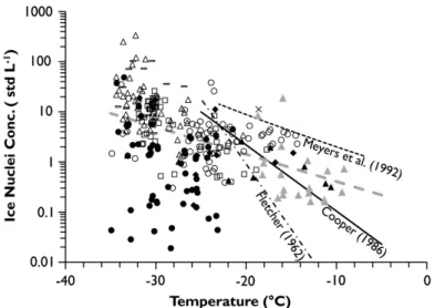
Figure 2.1:

IN number concentrations active at saturations with respect to liquid or above versus temperature (from

and spanning in total 12 years (symbols). Also included are common simplified parameterizations (see Chap. 2.2 for a definition) for IN number concentration as a function of temperature from three studies (black lines). The dashed grey line depicts a temperature-dependent fit to all data.

saturation vapour pressure due to the amount of solute dissolved (Raoult’s Law) and due to the curvature of the droplet (Kelvin effect) is described by Köhler theory (Pruppacher and Klett, 1997). Since usually a sufficient number of CCN

is available in the atmosphere, high supersaturation rates with respect to liquid phase only very rarely occur in nature, and homogeneous nucleation therefore does not play a role. Rather, heterogeneous nucleation dominates.

For ice nucleation, this is different. Only few particles suitable as IN exist in the atmo- sphere, so that supercooled droplets are common. Rogers et al. (1998) state that only 1 in 10

ambient particles are suitable as IN. Lamb and Verlinde (2012) give 1 l

as a typical IN concentration at −20 °C; for approximately every 4 °C decrease in temperature, IN concen- tration increases by a factor of ten (Fletcher, 1962). The number of IN activated at a specific temperature varies greatly with location and time (DeMott et al., 2010), as demonstrated in Fig. 2.1.

For pure water droplets, homogeneous ice nucleation does not occur down to a temperature of approximately −40 °C. For solution droplets (liquid aerosols), homogeneous ice nu- cleation occurs at warmer temperatures, because the solute depresses the freezing point of the liquid. Liquid aerosols especially suitable for homogeneous ice nucleation are sulfates, sulfates internally mixed with organics, and potassium (DeMott et al., 2003), though their homogeneous ice nucleation ability changes with solution droplet size and water accomo- dation coefficient of the solute (Kärcher and Koop, 2005). Throughout the present study, the two types of homogeneous nucleation (of pure water droplet and of liquid aerosols)

‡

CCN concentrations in the atmosphere vary with supersaturation with respect to liquid phase, air mass

origin, height, and time of day and range from 10 to 10

cm

(Wallace and Hobbs, 1977).

will be termed homogeneous nucleation and homogeneous nucleation of liquid aerosols.

Homogeneous ice nucleation through direct deposition does not occur in nature, since the required supersaturations with respect to frozen phase are never achieved.

In contrast to homogeneous ice nucleation, given the presence of suitable IN, heterogeneous ice nucleation already occurs at a few degrees below zero. Aerosols especially suitable as IN for heterogeneous ice nucleation are to current understanding mineral dust, fly ash, metalls, sulfates, and organics (DeMott et al., 2003). Rogers and Yau (1989) distinguish between four heterogeneous ice nucleation mechanisms:

• heterogeneous deposition (i. e. water vapour deposits directly onto an IN),

• condensation freezing (i. e. heterogeneous nucleation of a droplet followed by freez- ing),

• contact freezing (i. e. a supercooled droplet freezes spontaneously on contact with an IN), and

• immersion freezing (i. e. a supercooled droplet freezes after embedding an IN).

The latter two long prooved hard to distinguish since in both mechanisms an internal mix- ture of aerosol is required (Fornea et al., 2009). Heterogeneous deposition and contact freezing are to current understanding unimportant in cirrus formation, whereas immersion freezing is considered to be the most efficient heterogeneous ice nucleation mechanism in cirrus (Gierens, 2003). Apart from these classic heterogeneous ice nucleation mechnisms, others have been proposed which are still subject of controversy (Hoose and Möhler, 2012).

In nature, both homogeneous and heterogeneous ice nucleation occur. Notable homoge- neous ice nucleation requires low temperatures and strong updrafts and produces compar- atively small but numerous ice crystals. Notable heterogeneous ice nucleation already oc- curs at much higher temperatures and in weaker updrafts and produces larger but fewer ice crystals. However, for some combination of ambient air temperature, vertical velocity, and available IN, both ice nucleation processes can occur simultaneously and they then compete for the available water vapour (Ren and MacKenzie, 2005).

Ice formation in general is a complex process and the chemical and physical principles underlying it are still poorly understood (Cantrell and Heymsfield, 2005). Besides, ice formation also depends on macrophysical parameters such as cloud temperature, cloud type, cloud age, and radiation.

Growth processes and precipitation formation

Once a stable droplet or ice crystal is generated, various processes can lead to further growth

and finally precipitation production. In general, precipitation forms when a usually stable

cloud environment becomes unstable, that is when some droplets or ice crystals grow at the

expense of others. It is commonly distinguished between the warm rain process, in which

liquid water particles interact with water vapour and other liquid water particles, and cold rain processes, where frozen water particles are involved in the interaction. Generally, the probability for precipitation increases with cloud age, temperature, and vertical extent.

Warm rain process

In the warm rain process, droplet growth can occur in two ways. Firstly, by ongoing dif- fusional growth from water vapour. This process is very slow and does not lead to drop formation in realistic time. Secondly, droplets can grow through the classical collision- coalescence mechanism. In this mechanism, precipitation is formed by collision of droplets with each other and subsequent coalescence (i. e. sticking together/merging), resulting in fewer but larger droplets. This basic particle growth mechanism exists in many varieties. In the warm rain process, three basic processes lead to the production of large drops. First, au- toconversion

, the initial stage of the collision-coalescence process, leads to the formation of larger droplets (diameter ∼ 40 µm) and eventually drizzle drops (diameter ∼ 0.1 mm) through the collision and coalescence of small droplets (diameter ∼ 20 µm). Second, once the drops are larger and have already begun to fall (i. e. have become drizzle drops), accre- tion commences: falling drops grow after collision and coalescence with non-precipitating droplets. Third, once enough large drops are available, large hydrometeor self-collection rapidly adds to large drop production. However, drop size is limited, since at diameters larger than approximately 6 mm the drops become unstable und drop break-up occurs, pro- ducing new small droplets.

For falling drops to actually become precipitation, their sedimentation rate (i. e. fall of hy- drometeor relative to ambient air) has to exceed their evaporation rate, enabling them to reach the ground before evaporating completely. The fall velocity of liquid precipitation varies with particle size and ranges from 0.2 m s

to nearly 10 m s

(Khvorostyanow and Curry, 2001). The warm rain process dominates in the tropics, but also plays a role in mid-latitudinal mixed phase clouds.

Cold rain processes

Compared to the warm rain process, cold rain processes are far more complex and diverse.

The initial cold rain process is depositional (diffusional) growth of ice crystals. If droplets exist, then the diffusional growth occurs at the expense of these droplets. The reason is the smaller equilibrium vapour pressure over frozen water in comparison to over liquid water.

In such an environment, ice crystals will grow by diffusion of water vapour and supercooled droplets will evaporate to compensate for this. This process is referred to as the Bergeron- Findeisen process

(Korolev, 2006). In contrast to diffusional growth of droplets in the warm rain process, the diffusional growth of ice crystals in the cold rain processes is faster and can alone account for precipitation formation.

§

Note that the term autoconversion is sometimes also applied to drops or even ice crystals rather than merely droplets.

¶

The Bergeron-Findeisen process is sometimes also referred to as the Wegener-Bergeron-Findeisen,

Bergeron-Findeisen-Wegener, or simply ice phase process or theory.

When the ice crystals become larger, various other processes (apart from ongoing deposi- tional growth) add to their further growth. Collision with supercooled droplets followed by rapid freezing is called riming and results in the production of rimed ice crystals, then grau- pel, and eventually (in case of a slow freezing pace and strong updrafts) hail. Collision of ice crystals with other ice crystals followed by sticking together is called aggregation and results in the formation of snowflakes (aggregates). Aggregation is especially important near the melting layer, where the sticking efficiency is higher due to the liquid coating of the melting ice crystals.

Once a frozen particle has grown large enough for its fall velocity to exceed the upward ve- locity of the ambient air, sedimentation begins. As in the warm rain process, accretion may occur: falling snowflakes grow after collision with non-precipitating ice crystals. Should the frozen particle fall below the 0 °C level, melting occurs. Dependent on ambient air tem- perature and particle diameter, the particle may either reach the ground before thoroughly melting and fall as frozen precipitation (e. g. snow, graupel, hail) or it may have melted completely and fall as rain. For melting hailstones and graupel, depending on the thickness of their liquid coating and their fall speed, shedding may occur: the liquid coating is shed off as raindrops. The fall velocity of frozen precipitation varies greatly with particle size and habit and ranges from 0.2 m s

for small needles to several tens of m s

for large hailstones.

Ice enhancement

So far, all introduced processes were based on the so-called primary ice production mecha- nisms, on homogeneous and heterogeneous ice nucleation. However, observational studies show that in nature, the development of an ice crystal population in a cloud occurs at much higher speeds than these processes alone would enable and that the concentration of ice crystals exceeds the concentration of IN by orders of magnitude. This suggests additional mechanisms, which act as multipliers of the ice crystals produced by the primary ice pro- duction mechanisms and are hence referred to as secondary ice production mechanisms or ice enhancement mechanisms. These are not yet fully understood and a topic of ongo- ing research (e. g. Fridlind et al., 2007). So far, several theories have been suggested and are deemed more or less likely and effective in nature (Cantrell and Heymsfield, 2005).

Some proposed mechanisms are: fracture of ice crystals after collision, fragmentation of ice crystals during evaporation, shattering of large drops during freezing, and splintering of ice crystals during riming, also referred to as rime-splintering or Hallett-Mossop process (Hallett and Mossop, 1974; Saunders and Hosseini, 2001).

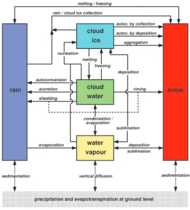
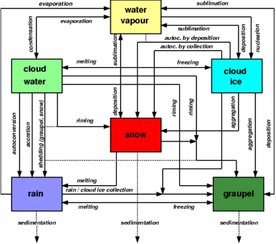
An overview of all described cloud microphysical processes is depicted in Fig. 2.2. Though

for a single particle the above mentioned microphysical processes occur successively, in

the life cycle of a natural cloud, consisting of a whole particle population (up to 800 cm

for continental storm clouds; Rogers and Yau, 1989), several or all of these processes occur

simultaneously. Furthermore, the processes compete for available water vapour. Therefore,

these processes are difficult or impossible to discriminate in the model world. For example,

Figure 2.2:

Schematic to illustrate the various cloud microphysical processes (based on

when shedding occurs, the falling liquid-coated particle will also collect droplets during its fall, thereby thickening its liquid coating. This additional liquid water is shedd off as drops, too. These drops in turn, are re-collected by other falling liquid-coated particles.

How atmospheric models can nevertheless handle this multitude of intertwined processes, or at least approximate them, is described in the following section.

2.2 Cloud microphysics in NWP models

The complex nature of cloud microphysics cannot be fully captured by NWP models,

for two reasons. Firstly, the understanding of all processes involved is still incomplete

(Heintzenberg and Carlson, 2009), as demonstrated in the previous section. Secondly, even

the known processes cannot all be implemented into the models. Due to limited compu-

tational power, models have a far coarser resolution (several km) than would be necessary

to resolve cloud microphysical processes explicitely (a few µm). In relation to the model

grid, cloud microphysical processes occur at subgrid-scale and need to be parameterized. A

parameterization is the description of a subgrid-scale process with the predicted grid-scale

parameters of a model, and the determination of the temporal changes of these grid-scale

parameters due to the subgrid-scale process. In short, it is the formulation of the ensemble

Figure 2.3:

Average PSDs plotted in 10 °C temperature increments. The dots show one standard deviation above average value/bin. From

effect of subgrid-scale processes on the resolved grid-scale variables (Doms et al., 2011).

Since it is the ensemble effect rather than the effect of a single particle that is of interest for

model cloud microphysics, the first and most basic assumption made in a model is to group

the multitude of various hydrometeors into a few distinct hydrometeor classes. The more

hydrometeor classes, the more complex the scheme. Second, the model needs to describe

the members of such a hydrometeor class. Most microphysical processes depend very much

on particle shape and size, that is the PSD has a strong impact on the overall evolution of the

cloud as a whole. The description of the members of the hydrometeor classes is commonly

done through the choice of a characteristic mass-size relation which gives the mass m as a

function of diameter D (Eq. 2.1) and an appropriate PSD, which gives the number density

N of particles as a function of diameter D (Eq. 2.2). The chosen PSD is usually based on

observed PSDs and could, for example, be monodisperse, exponential, gamma, or any other

reasonable mathematical function f (D). Finding a good fit to observed PSDs is a challeng-

ing task, since observed PSDs exhibit a large spread. Exemplarily, PSDs for convective and

stratiform cloud situations from 10 field campaigns are depicted in Fig. 2.3 from Heymsfield

et al. (2013). How the fit of different mathematical functions to an observed PSD varies

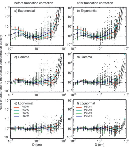
Figure 2.4:

Ratio of observed to theoretical number concentration for three distribution types on 31 July 2007. Before (left) and after truncation correction (right). Thick black line: geometric mean.

Thin black lines: one standard deviation above and below mean. From

is depicted for one case study in Fig. 2.4 from Tian et al. (2010). For cirrus clouds, the authors find the lognormal function to provide the best fit to observed PSDs. Exactly which hydrometeor classes and which corresponding PSDs the models evaluated in the present study use, is described in detail in Chap. 3.

m

(D) = α

· D

(2.1)

N

(D) = f

(D), (2.2)

where α (in kg m

) and β (dimensionless) are coefficients dependent on hydrometeor class x.

Total water mass remains the same, though the water mass of one hydrometeor class may in-

crease (decrease) at the expense (in favour) of another. The water mass in each hydrometeor

class is mathematically described by budget equations, taken together commonly referred to as the water-continuity model. Basically, two approaches exist to implement this into a NWP model: spectral water-continuity models and bulk water-continuity models.

Spectral water-continuity models are the most direct approach for representing cloud mi- crophysics in a NWP model. Each hydrometeor class is subdivided according to particle size. The number of particles per size bin (the particle number concentration) N

(D) is pre- dicted using budget equations. The total number density of a hydrometeor class N

is then calculated by integrating over the whole PSD. The total mass fraction (or specific content) q

of a hydrometeor class x is calculated by integrating over the mass of the particles in each size bin. Thus, spectral water-continuity models directly predict the PSD, and from this diagnose the total number density N

and total mass fraction q

. These are simply proportional to the zeroth M

and third moment M

of the PSD (Eq. 2.3-2.5).

M

= Z

0

D

· N(D) dD (2.3)

N

= Z

0

N

(D) dD ∼ M

(2.4)

q

= 1 ρ ·

Z

0

m

(D) · N

(D) dD ∼ M

, (2.5)

where n is the order of moment M ^{and ρ} is the ambient air density. Since the accuracy of spectral water-continuity models depends on a sufficiently large number of bins per hy- drometeor class, these models quickly become complicated and computationally expensive.

Therefore, though being very detailed, they are not suitable for NWP model application.

Bulk water continuity-models aim at minimizing the number of equations by reducing the number of hydrometeor classes to a minimum and by predicting their respective total mass fraction directly. For this, assumptions on particle shape and PSD are needed. In contrast to the spectral water-continuity models, the moments (or rather parameters proportional to the moments, e. g. total mass fraction q

) are predicted with budget equations and the shape of the PSD is diagnosed from these. This requires the assumption, that the evolution of a PSD can be approximated by varying the free parameters of the mathematical function f (D) as- sumed for the PSD. These free parameters are related to the moments of the PSD. Standard bulk water-continuity models for NWP application are one-moment schemes, which, as the name suggests, merely predict one moment, usually the total mass fraction q

(Eq. 2.5). A two-moment scheme additionally predicts another moment, usually the total number con- centration N

(Eq. 2.2). Though multi-moment schemes are possible, they are currently only used in research (e. g. Lim and Hong, 2010; Thompson et al., 2008; Seifert and Be- heng, 2006), since doubling the predicted moments means doubling the number of included prognostic variables, which increases computational costs drastically.

As stated above, the microphysical processes and their feedbacks are represented by budget

equations, with which the respective parameters are predicted. For a one-moment bulk

water-continuity model the budget equation for the total mass fraction q

in advection form is

∂q

∂t +~ v · ∇q

− 1 ρ

∂P

∂z = S

− 1

ρ ∇ · ~ F

, (2.6)

with the three-dimensional wind vector ~ v and the density of moist air ρ. The budget equa- tion consists of five terms: the temporal evolution of the total mass fraction q

plus the advection of q

and the vertical divergence of the precipitation fluxes P

equal the cloud microphysical sources and sinks (or transfer rates) S

and the turbulent fluxes ~ F

. The pre- cipitation fluxes depend on the terminal fall speed of the particle, which in turn depends on q

. For non-precipitating hydrometeor classes, terminal fall speed is negligible and the pre- cipitation flux term is commonly set to zero and neglected. For precipitating hydrometeor classes, the turbulent flux term is commonly neglected, since it is small in comparison to the precipitation flux term.

In the following chapter, the cloud microphysical schemes currently in use at DWD are

reviewed. The cloud microphysical schemes of the model versions evaluated in the present

study are described in the respective model chapters.

The operational NWP system at DWD currently consists of a chain of three models nested into each other: the global model GME and the regional models COSMO-EU and COSMO- DE. Within the process of model development, model versions which actually enter oper- ational service receive an official release version number. Prior to becoming operational, new model versions undergo extensive tests. Once these new versions are close to becom- ing operational, the runs performed with them are stored in DWD’s database under a unique experiment number, enabling their discrimination.

The present study evaluates two models of DWD’s model chain, GME and COSMO-DE.

The models themselves and the experimental versions of them are introduced in the follow- ing sections.

3.1 GME

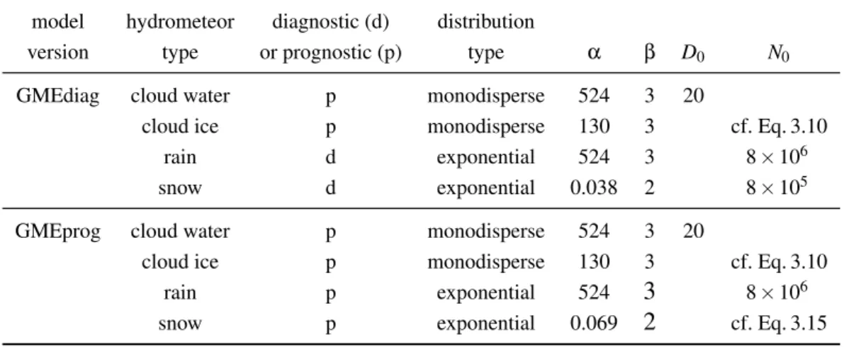
In the following, the GME model with its general aspects and particularly its microphysics is described. Since the present study compares two versions of the model, emphasis is laid on describing the differences between the two versions. At the end of the chapter, Table 3.3 summarizes the most important microphysical parameters of the model versions.

For a more comprehensive introduction to GME see Majewski et al. (2002) and Schulz and Schättler (2011). For details on the cloud microphysical parameterizations see Doms et al.

(2011).

3.1.1 General aspects

GME (Majewski et al., 2002) is the global NWP model of DWD. Operational since 1 De- cember 1999, it is a hydrostatic model of the atmosphere and delivers the boundary condi- tions for the regional scale models COSMO-EU and COSMO-DE. The primitive equations are solved using a finite-difference method on a hexagonal icosahedral A-grid (cf. Fig. 3.1).

GME uses terrain-following coordinates in the vertical, which are defined via the time- dependent surface pressure and are smoothed out towards the stratosphere (hybrid coordi- nates). Thus, level thickness varies with time. The GME versions evaluated in this study all have a mean horizontal grid size of 40 km

and 40 hybrid levels in the vertical. Level thick- ness ranges approximately from 25 m at the Earth’s surface, 550 m in 5 km height, to 750 m in 10 km height. Forecasts are available in hourly resolution and the model is initialized four times a day (at 0, 6, 12, and 18 UTC). The model is initialized using a three-dimensional variational data assimilation system. GME assimilates observations of geopotential, hor- izontal wind vector, temperature, sea surface temperature, relative humidity, snow cover, snow depth, fraction of fresh snow, sea ice cover, and ozone mixing ratio. The observations stem from synoptic stations, drifting buoy, radiosondes, polar-orbiting and geostationary satellites, and aircrafts (Wergen and Buchhold, 2002; Majewski et al., 2002) .

In addition to resolved (i. e. grid-scale) clouds which are parameterized by microphysi- cal schemes, GME also provides information from within a grid-box (i. e. subgrid-scale) for several applications (e. g. cloud fraction) and as input for other parts of the model (e. g. radiation scheme). In the following, the grid-scale cloud scheme, that is the micro- physical parameterization of the model, is explained in detail.

*

The to-date operational version has an increased horizontal resolution of 30 km.

Figure 3.1:

Model domain and horizontal grid structure of GME (from

3.1.2 Cloud microphysics: Two-category ice scheme

Grid-scale precipitation in GME and the associated cloud microphysical interactions are formulated as a bulk scheme (see Chap. 2.2 for a general introduction to bulk schemes).

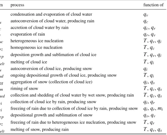
GME distinguishes between precipitating and non-precipitating hydrometeor classes, fea- turing in total four hydrometeor classes: First, cloud water (index x = c), which is defined as droplets suspended in the air, with diameters smaller than 100 µm and no remarkable mo- tion relative to the air flow. Second, cloud ice (index x = i), defined similar to cloud water, but for frozen phase. Third, rain (index x = r), which consists of comparably large drops, with diameters ranging from 100 to 8000 µm and size-dependent fall speed relative to the ambient air flow. Fourth, snow (index x = s), treated as large, slightly rimed ice crystals and aggregates of ice crystals, also with size-dependent fall speed relative to the ambient air flow. Owing to the number of frozen phase hydrometeor classes, this scheme is commonly referred to as the two-category ice scheme.

The particles in these four hydrometeor classes interact through various cloud microphysi- cal processes which are formulated as a function of the specific contents q

of the hydrom- eteor classes. Figure 3.2 gives a schematic overview of the hydrometeor classes and the

Figure 3.2:

Microphysical processes of cloud and precipitation generation in the two-category ice scheme

of DWD (from

exception of the condensation and evaporation of cloud water

and the depositional growth

and sublimation of snow

, which are positive for condensation/deposition and negative for

evaporation/sublimation.

Table 3.1:

Sources and sinks in the two-category ice scheme of DWD and their dependency on predicted model variables.

term process function of

S

condensation and evaporation of cloud water q

S

autoconversion of cloud water, producing rain q

S

accretion of cloud water by rain q

, q

S

evaporation of rain q

, q

S

heterogeneous ice nucleation T , q

, q

S

homogeneous ice nucleation T , q

S

deposition growth and sublimation of cloud ice T , q

, q

S

melting of cloud ice T , q

S

autoconversion of cloud ice, producing snow q

S

ongoing depositional growth of cloud ice, producing snow T , q

S

aggregation of snow (collection of cloud ice) q

, q

S

riming of snow T , q

, q

S

collection and shedding of cloud water by wet snow, producing rain T , q

, q

S

collection of cloud ice by rain, producing snow q

, q

S

freezing of rain due to collection of cloud ice by rain, producing snow q

, q

, m

S

depositional growth and sublimation of snow q

, q

S

freezing of rain due to heterogeneous ice nucleation, producing snow T , q

S

melting of snow, producing rain T , q

, q

interaction processes as parameterized in DWD’s two-category ice scheme, which is imple- mented in GME. As stated in Chap. 2.2, though undergoing changes regarding a particular hydrometeor class, in total, water mass remains constant. Table 3.1 lists all parameterized sources and sinks S, and additionally gives the model parameters of which they are de- pendent. Equations 3.1–3.5 show how conservation of total mass is ensured, and how the source and sink terms add to the water mass of each hydrometeor class. All conversion terms are defined positive, with exception of the condensation and evaporation of cloud water S

and the depositional growth and sublimation of snow S

, which are positive for condensation/deposition and negative for evaporation/sublimation.

S

= −S

+ S

− S

− S

− S

(3.1)

S

= S

− S

− S

− S

+ S

− S

− S

(3.2)

S

= S

+ S

+ S

− S

− S

− S

− S

− S

(3.3)

S

= S

+ S

− S

+ S

− S

− S

+ S

(3.4)

S

= S

+ S

+ S

+ S

+ S

+ S

+ S

+ S

− S

(3.5)

The transfer rate for condensation and evaporation S

is obtained by saturation adjustment:

it is assumed that in case of supersaturation with respect to liquid phase a sufficient number of CCN is always present, enabling the formation of cloud droplets. Heterogeneous ice nu- cleation through heterogeneous deposition S

is parameterized by a simple temperature- dependent relation following Fletcher (1962). For temperatures below −25 °C, supersatu- ration with respect to frozen phase is sufficient for heterogeneous deposition to occur. For temperatures between −25 °C and −6 °C, supersaturation with respect to liquid phase is required, too. In both cases, no cloud ice is yet allowed to be present (q

= 0). Exem- plarily, the source and sink term for heterogeneous ice nucleation S

is given in Eq. 3.6.

For the exact formulations of all other source and sink terms it is referred to the model documentation (Doms et al., 2011).

S

= ρ

· m

· ∆t

N

(T ) (3.6) Homogeneous ice nucleation S

of all cloud water instantaneously sets in for temperatures below −37 °C. Note that homogeneous freezing in this scheme refers to freezing of pure water only and does not include homogeneous ice nucleation of liquid aerosols.

Once pristine ice crystals exist, they can continue to grow (or shrink away) by water vapour deposition (cloud ice sublimation) S

, which sets in for supersaturation (subsaturation) with respect to frozen phase. This depends on the number concentration of cloud ice par- ticles N

(T ) which in turn is temperature dependent (how the number concentrations N

are parameterized is explained in detail in the respective sections of the model versions).

To avoid unnaturally large ice crystals, their size is limited to a maximum diameter of

∼ 200 µm.

Rain production through autoconversion of cloud water S

is parameterized as a function of the specific content of cloud water q

without any autoconversion thresholds. Snow pro- duction through autoconversion of cloud ice S

is parameterized in similar manner. Snow production through further depositional growth of cloud ice S

is dependent on the time scale for cloud ice to grow to snow of initial snow mass 3 × 10

kg (corresponding to a minimum snowflake diameter of ∼ 300 µm). Further mass increase of rain by accretion S

and further mass increase of snow by aggregation S

is included. For temperatures below (above) freezing level riming of snow (shedding) S

(S

) occurs. Note that in the cloud microphysical scheme of the model, the term shedding is not used in the sense of liquid- coated frozen particles shedding the liquid layer off as rain, as introduced in Chap. 2.1.

Rather, it is the collection of cloud water by falling, melting snow and the subsequent shed- ding off of this liquid coating as rain. The collision of supercooled rain with cloud ice leads to instantaneous freezing of the rain which is from then on considered to be snow.

This snow production process involves two sinks since it firstly decreases cloud ice S

and

secondly decreases rain S

. Two diffusional growth processes are parameterized: evapo-

ration of rain S

and deposition/sublimation of snow S

. The latter is defined positive

for deposition. Melting of cloud ice S

occurs instantaneously when temperature rises

above 0 °C. Melting of snow S

occurs gradually when temperature rises above 0 °C.