Efficient Elimination of the Basis Set Superposition Error

Superposition Error

Inaugural-Dissertation zur

Erlangung des Doktorgrades

der Mathematisch-Naturwissenschaftlichen Fakultät der Universität zu Köln

vorgelegt von Katarzyna Walczak aus Ostrów Wielkopolski

Köln

2012

Priv.-Doz. Dr. M. Hanrath

Tag der mündlichen Prüfung: 15.06.2012

gifted for something and that this thing must be attained.

Maria Skłodowska-Curie

Der Basissatzsuperpositionsfehler (BSSE) stellt eines der größten Hindernisse in quantenchemischen Berechnungen dar, die eine genaue Berechnung von Wechsel- wirkungsenergien anstreben. Die Bedeutung eines BSSE Eliminierungsverfahrens ist unter anderem darin begründet, dass der BSSE in der Größenordnung der zu berech- nenden Wechselwirkungsenergie liegen kann und daher die Genauigkeit dieser sig- nifikant beeinträchtigt.

In der vorliegenden Arbeit werden neue Ansätze vorgestellt, um den BSSE in wellen- funktionsbasierten quantenchemischen Rechnungen an großen molekularen Clustern effizient zu eliminieren. Die Anwendbarkeit der Methoden wurde ausführlich unter anderem an Wasser Clustern diskutiert, deren Größe sich von einem Wasser-Dimer bis hin zu einem (H

O)

Cluster erstreckte. Eine Übersicht über die in der Lite- ratur bekannten BSSE Eliminierungsverfahren wird ebenfalls dargestellt und die hier vorgestellten Methoden werden damit verglichen.

Die neu vorgestellten Verfahren bieten mit nur geringeren Einbußen in der Genauigkeit der Rechnungen einen sehr effizienten Weg BSSE korrigierte Wechselwirkungsen- ergien zu erhalten, welche sogar teilweise mit den verfügbaren Standardmethoden auf- grund der Systemgröße nicht mehr zugänglich wären.

vii

The basis set superposition error (BSSE) is one of the major obstacle occuring in quan- tum chemical calculations which aim at a accurately prediction of interaction energies.

The importance of a BSSE elimination procedure is among other things manifasted by the fact, that the magnitude of the BSSE can be as large as the interaction energy itself, affecting the accuracy of the calculated interaction energies therefore significantly.

In this work new approaches to eliminate the BSSE efficiently from wavefunction based quantum chemical calculations on large molecular clusters are presented. The applicability of these schemes is studied in great detail among others on a water clus- ter series ranging in size from a water dimer up to even a (H

O)

water cluster. An overview of the correction schemes known from the literature is also given and the newly developed schemes are compared with the literature ones.

The presented schemes allow to account with only small loss in accuracy very effi- ciently for BSSE corrected interaction energies, which are partly no more feasible to calculate with standard methods due to the large system size.

ix

Kurzzusammenfassung vii

Abstract ix

1 Introduction 3

2 Theory 5

2.1 Methods of Quantum Chemistry . . . . 5

2.1.1 Hartree-Fock Theory . . . . 5

2.1.2 Perturbation Theory . . . . 9

2.1.3 Coupled-Cluster Theory . . . . 11

2.1.4 Explicitly correlated methods . . . . 13

2.2 Incremental Scheme . . . . 15

2.3 Basis Set Superposition Error . . . . 22

3 Results and Discussion 25 3.1 Incremental evaluation of interaction energies . . . . 25

3.1.1 Introduction . . . . 25

3.1.2 Applications . . . . 32

3.2 BSSE correction schemes for n-body clusters . . . . 42

3.2.1 SSFC, PAFC and VMFC schemes . . . . 42

3.2.2 Approximate SSFC(R) and VMFC(2)(R) . . . . 45

3.2.3 Approximate SSFC

scheme . . . . 47

3.2.4 Approximate SSFC(S) scheme . . . . 48

3.3 Applications . . . . 50

3.3.1 Comparison of the SSFC, PAFC and VMFC(2) schemes . . . 52

3.3.2 Approximate SSFC(R) scheme applied to water clusters . . . 55

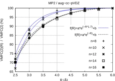
3.3.3 Approximate SSFC(R) scheme applied to methanol clusters . 61 3.3.4 Basis set dependency on the approximate SSFC(R) scheme . . 62

i

3.3.5 SSFC(R) corrected stabilization energies of the water cluster

series . . . . 65

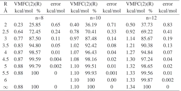
3.3.6 Approximate VMFC(2)(R) scheme . . . . 71

3.3.7 Approximate SSFC

scheme . . . . 74

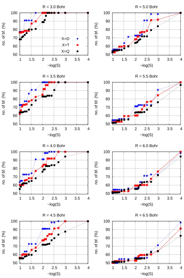
3.3.8 Approximate SSFC(S) scheme . . . . 82

3.4 Incremental evaluation of core, core-valence and valence correlation energies . . . 111

3.4.1 Introduction . . . 111

3.4.2 Applications . . . 112

4 Conclusion 131

A MP2 and CCSD incremental interaction energies 133

B SSFC(R), VMFC(2)(R) and SSFC(S) results at the MP2 and CCSD levels

of theory 143

C Core, core-valence and valence correlation energies 155

Literature 157

Danksagung 165

Erklärung gemäß §4 Abs. 9 der Promotionsordnung 167

Å Ångstrøm AO atomic orbital a.u. atomic unit

avg. average

BDE bond dissociation energy bf. basis function

bfs. basis functions

BO Born-Oppenheimer

BSSE basis set superposition error ca. approximately

CABS complementary auxiliary basis set

cal calorie

CBAS auxiliary basis set CBS complete basis set CC coupled cluster (method)

CCSD(T) coupled cluster method with singles and doubles and a perturbative es- timate of triples

cf. compare

CI configuration interaction (method) CP counterpoise (correction)

CPU central processing unit

D

dissociation energy from the potential minimum DFT density functional theory

DKH Douglas–Kroll–Hess (Hamiltonian)

DZ double-ζ

E energy

e.g. for example

ECP effective core potential edn. edition

ed.; eds. editor; editors

1

ǫ

one-electron orbital energy

eq. equation

et al. and others etc. and so forth f ˆ Fock operator

g g-factor

g

nuclear g-factor GTO Gaussian-type-orbital H ˆ Hamilton operator HF Hartree–Fock (method) i.e. that is

J Joule

J ˆ

Coulomb operator K ˆ

Exchange operator k kilo (10

)

LCAO linear combination of atomic orbitals log logarithm to the base 10

MO molecular orbital m.r.e. mean relative error

MP2 second-order Møller–Plesset perturbation theory

no. number

PEC potential energy curve PES potential energy surface PT perturbation theory PP pseudopotential

QZ quadruple-ζ

RI resolution of identity (approximation) SCF self-consistent field (method)

SD Slater determinant STO Slater-type-orbital TS transition-state

TZ triple-ζ

vide infra see below

vs. versus

ZPVE zero-point vibrational energy

Z

atomic number of nucleus I

Introduction

For the accurate evaluation of weak intermolecular interactions one has to apply high level quantum chemical methods such as the coupled-cluster (CC) approach or Møller- Plesset (MP) perturbation theory. The main drawback of the wavefunction-based cor- relation methods is the strong dependence of their demand of computational resources on the size of the one-particle basis set. For small clusters these calculations can be done routinely with commercially available quantum chemical software, however for large clusters in combination with large basis sets - which are clearly necessary for an accurate description - the application of CCSD(T) or even CCSD becomes quickly very time consuming or impossible at all. Even the calculations of error measures such as the basis set superposition error (BSSE, vide infra) becomes a difficult task for large clusters. In this work different approximations to account for the BSSE correc- tions for large clusters at high correlation level are introduced and compared among each other with respect to their efficiency. Furthermore the incremental scheme, which is a method from the large field of the so-called local correlation methods is applied to account for correlation energies of large water cluster and other systems.

3

Theory

2.1 Methods of Quantum Chemistry

2.1.1 Hartree-Fock Theory

The Schrödinger equation 2.1 (here in its time-independent form):

HΨ = ˆ EΨ, (2.1)

is not soluble in closed form for the most systems of chemical interest. Thus it is therefore necessary to introduce approximations. The Hartree-Fock (HF) [1,2] approx- imation is central to computational chemistry, its outcome is exploited as the starting point for an more accurate solution to the Schrödinger equation. Within the HF theory as described below relativistic effects are neglected and the Born-Oppenheimer (BO) approximation is used, treating the nuclei as stationary sources of electrostatic fields.

From the BO model follows, that the nuclear kinetic energy is neglected, correlation in the attractive electron-nuclear potential term is eliminated, and the repulsive nuclear- nuclear potential energy term ˆ h

(vide infra, Eq. 2.3) becomes constant for a given geometry. Thus for the electronic Schrödinger equation:

H ˆ

Ψ

= EΨ

, (2.2)

the electronic Hamiltonian for a n-electron wave function can be written in terms of one-, two-, zero-electron terms as:

H ˆ

=

n

X

i

h ˆ

+

n

X

i<j

ˆ

g

+ ˆ h

(2.3)

5

and reads in atomic units (a.u.) with the omission of the trivial additive constant ˆ h

for fixed nuclear positions:

H ˆ

= −

n

X

i

1 2 ∇

−

n

X

i M

X

I

Z

r

+

n

X

i<j

1 r

. (2.4)

In the HF theory [3] the electronic wave function, describing the ground state of an n-electron system is approximated by a single Slater determinant (SD). A SD is an antisymmetrized product of one-electron wave functions called spin orbitals ϕ

, which depend upon spatial coordinates r

= {x

, y

, z

} and a spin part α or β:

Ψ

= C AΘ = ˆ C A ˆ

n

Y

i=1

ϕ

(i). (2.5)

The normalization constant C equals (n!)

when the spin orbitals are orthonormal (vide infra, Eq. 2.10), A ˆ is the antrisymmetrize operator and the one-electron wave function product Θ is called Hartree product. Eq. 2.5 satisfies two fundamental re- quirements of quantum mechanics. First the indistinguishability of electrons is ensured and second the wave function is antisymmetric with respect to interchange of the co- ordinates of any two electrons. The second statement is known as the Pauli principle, the crucial quantity in Eq. 2.5 regarding the Pauli exclusion is the antrisymmetrizer:

A ˆ =

n!

X

k=1

(−1)

P ˆ

, (2.6)

where the sum runs over the n! possible Hartree products, P ˆ

is the permutation op- erator and (−1)

describes the parity of the k-th permutation (equals either 1 of -1, depending on whether an even or odd number of permutations will be necessary).

The variational method [4] is utilized to solve Eq. 2.2 approximately, for arbitrary functions Φ we have:

E[Φ] = hΦ| H ˆ

|Φi

hΦ|Φi ≥ E ˜

, (2.7) with E ˜

being the exact ground state energy. Minimization of E[Φ] for a reasonable ansatz Φ leads to a approximate ground state energy, which is larger or in best case equal to E ˜

. If the energy functional (i.e., the expectation value) is stationary with respect to all possible variations δ

in the function Φ, then Φ is the searched solution:

δ

E[Φ] = 0 (2.8)

Having selected a single determinant trial wave function, the variational principle can

be then applied to derive the HF equations by minimizing the expectation value with

respect to the choice of spin orbitals:

min : E

[{ϕ

}] =

hΨ

| H ˆ

|Ψ

i (2.9) Choosing the spin orbitals to be orthonormal:

Z

ϕ

ϕ

dτ = δ

(2.10)

one can evaluate the matrix elements over one- and two-electron operators using the Slater-Condon rules [5]. The expectation value from Eq. 2.9 may be simplified to:

hΨ

| H ˆ

|Ψ

i =

n

X

i=1

hϕ

| h|ϕ ˆ

i + 1 2

n

X

i,j

hϕ

ϕ

|ˆ g|ϕ

ϕ

i − hϕ

ϕ

|ˆ g|ϕ

ϕ

i

=

n

X

i=1

hϕ

| h|ϕ ˆ

i + 1 2

n

X

i,j

hϕ

| J ˆ

− K ˆ

|ϕ

i

(2.11)

The electron-electron interaction are represented via the Coulomb J ˆ

and exchange operator K ˆ

, both defined by their effects when operating on a spin orbital ϕ

:

J ˆ

(1)ϕ

(1) =

Z ϕ

(2)ϕ

(2) r

dτ

ϕ

(1) (2.12)

K ˆ

(1)ϕ

(1) =

Z ϕ

(2)ϕ

(2) r

dτ

)

ϕ

(1) (2.13)

Note that the Coulomb interaction will always survive spin integration, whereas the exchange interaction only occurs between electrons having the same spin, the motion of electrons with parallel spins is therefore said to be correlated.

Applying the variational principle to the energy expression from Eq. 2.11 yields the HF equations:

ˆ h(1)ϕ

(1) + X

j

h J ˆ

(1) − K ˆ

(1) i

ϕ

(1) = ǫ

ϕ

(1), (2.14) where the Fock operator for electron (1):

f ˆ (1) = ˆ h(1) + v

(1) = ˆ h(1) + X

j

h J ˆ

(1) − K ˆ

(1) i

, (2.15)

is the sum of the core-Hamiltonian operator ˆ h(1) and an effective one-electron po- tential operator called the HF potential v

. The HF equations 2.14 may be written as:

f(1)ϕ ˆ

(1) = ǫ

ϕ

(1), (2.16)

1

Since the one-electron operator in case of the nonrelativistic Hamiltonian does not depend on spin,

spin integration also does not change the values of one-electron integrals.

which is an eigenvalue equation with the spin orbitals as eigenfunctions and the en- ergy of the spin orbitals as eigenvalues. The complicated many-electron problem has been replaced by a one-electron problem in which the electron-electron repulsion is accounted for in an average fashion. Each electron is considered to be moving in the field of the nuclei and the average field of the other (n-1) electrons, therefore the HF method is referred to as a mean-field approximation.

Roothaan [1,2] described matrix algebra equations that permitted HF calculations to be carried out using a basis set approximation for the unknown molecular orbitals (MO).

Each MO ϕ

(r) is expanded in terms of known basis functions χ

(r), conventionally called atomic orbitals (MO=LCAO, Linear Combination of Atomic Orbitals):

ϕ

(r) =

K

X

ν

c

χ

(r) i = 1, 2, ...K (2.17) If the set {χ

} was complete (infinite number of basis function), this would be an exact expansion. As the basis set approaches completeness, one approaches the HF-limit (numerical HF solution), what is for practical computational reasons not reachable.

Substituting the linear expansion 2.17 into the HF equation 2.16 and multiplying by χ

on the left and integrating turns the coupled integro-differential HF equations into:

X

ν

F

C

= ǫ

X

ν

S

C

, (2.18)

which are known as Roothaan equations. The entire set of equations can be written as the single matrix equation:

FC = SCǫ. (2.19)

The S matrix contains the overlap of basis function, the Fock matrix F is the matrix representation of the Fock operator and depends on the expansion coefficients C:

F = F(C). (2.20)

The Roothaan equations are therefore nonlinear and they need to be solved iteratively.

In order to find the eigenvectors C and eigenvalues ǫ by diagonalizing F, the gener- alized matrix eigenvalue Eq. 2.20 should be transformed into a conventional form.

That means the overlap matrix must be unity, which is ensured when a transformed set of basis functions form an orthonormal set. One can choose a real and nonsingular transformation matrix X such that X

SX=1 and obtain:

F ˜ C ˜ = ˜ Cǫ with : ˜ F = X

FX and C ˜ = X

C, (2.21) where the matix X defines an orthonormal basis {φ

} expanded in the original basis {χ

}:

φ

(r) =

K

X

ν

χ

(r)X

(2.22)

Before the self-consistent field (SCF) procedure is carried out, the basis functions are orthogonalized by exemplary symmetric or canonical orthogonalization procedure [5].

During the SCF iteration one employs MO coefficients from a previous iteration as an orthonormal basis set.

2.1.2 Perturbation Theory

Another theory framework besides the variational principle used to solve the Schrödinger equation 2.1 is the so-called perturbation theory (PT) [2, 6]. The cru- cial characteristic within PT is that a solution of an approximate Schrödinger Eq. is known:

H ˆ

Φ

= E

Φ

i = 0, 1, 2, ...∞ , (2.23) and that this solution differs only slightly from the exact one. The exact Hamiltonian H ˆ is divided into a reference or unperturbed Hamilton operator H ˆ

and a perturbation operator H ˆ

:

H ˆ = ˆ H

+ λ H ˆ

, (2.24)

H ˆ

should closely represent the true Hamiltonian and for which the solutions form a complete set as indicated in Eq. 2.23. The perturbation operator H ˆ

should capture only a small fraction of the true Hamiltonian, so that the perturbation becomes small, in Eq. 2.24 λ is a dimensionless parameter that, as it varies from 0 to 1, maps H ˆ

into H ˆ

. The energy and wavefunction of Eq. 2.1 Ψ are expanded in form of a Taylor series in powers of the perturbation parameter:

E = E

+ λE

+ λ

E

+ ... + λ

E

+ ... (2.25) Ψ = Φ

+ λΦ

+ λ

Φ

+ ... + λ

Φ

+ ... , (2.26) where E

and Φ

are the p-th order correction to the reference energy E

and the reference wavefunction Φ

of the unperturbed system. Inserting Eqs. 2.24, 2.25 and 2.26 into the Schrödinger equation yields:

( ˆ H

+ λ H ˆ

)(Φ

+ λΦ

+ ...) = (E

+ λE

+ ...)(Φ

+ λΦ

+ ...) (2.27) Since all terms in 2.27 are linearly independent, we can collect terms with the same power of λ to:

(E

− H ˆ

)Φ

= ( ˆ H

− E

)Φ

−

p

X

k=2

E

Φ

(2.28)

Eq. 2.28 may be further simplified if intermediate normalization (the overlap of the

perturbed with unperturbed wave function is equal to unity) is supposed, which is

equivalent with:

hΦ

|Φ

i = 1 hΦ

|Φ

i = 0 for all p > 0 (2.29) and Eq. 2.28 may be simplified to:

E

= hΦ

| H ˆ

|Φ

i. (2.30) Since the solutions 2.23 to the unperturbed system 2.28 (to the zero order) generate a complete set of functions, one can expand the unknown higher order correction to the wave function in terms of these known functions:

Φ

= X

i

c

Φ

. (2.31)

The first-order energy correction can now be evaluated and is equal to the expectation value of the perturbation operator over the unperturbed wave function:

E

= hΦ

| H ˆ

|Φ

i. (2.32) The major outcome is that the higher order correction - to the energy and wavefunction - may also be expressed in terms of matix elements of the perturbation operator over unperturbed wave functions.

Møller and Plesset suggested using the sum over Fock operators for the unperturbed Hamiltonian:

H ˆ

= X

i

f ˆ

= X

i

ˆ h

+ X

j

( ˆ J

− K ˆ

)

= X

i

h ˆ

+ X

i

X

j

hˆ g

i = X

i

ˆ h

+ 2h V ˆ

i,

(2.33) in which the (average) electron-electron repulsion is counted twice. The perturbation operator returns the correct (electronic nonrelativistic) Hamiltonian and is therefore set to be the exact electron-electron repulsion operator V ˆ

minus twice the h V ˆ

i operator (which captures electron-electron repulsion as computed from summing over Fock operators):

H ˆ

= ˆ H − H ˆ

= X

i

X

j>i

ˆ

g

− X

i

X

j

hˆ g

i = ˆ V

− 2h V ˆ

i. (2.34) Since the zeroth-order wave function is the HF determinant, the zeroth-order energy in MP theory is the sum of MO energies:

E

= hΦ

| H ˆ

|Φ

i = hΦ

| X

i

f ˆ

|Φ

i = X

i

ǫ

. (2.35)

And the first-order energy correction is the negative of the over-counted electron- electron repulsion:

E

= hΦ

| H ˆ

|Φ

i = h V ˆ

i − 2h V ˆ

i = −h V ˆ

i. (2.36) Thus the HF energy is the energy corrected through first-order in Møller-Plesset per- turbation theory, exactly the sum of Eqs. 2.35 - 2.36. Electron correlation is therefore firstly accounted for when the MP second-order energy correction is evaluated. This involves the evaluation of all possible excited Slater determinants. But within a fi- nite basis set approximation, the ways to distribute the electrons in the HF orbitals are also limited and hence the number of excited determinants is finite what means that the many-electron wave function is truncated. From the Condon-Slater rules follows (since our perturbation operator is a two-electron operator) that only double and single excited determinants have to be considered. Furthermore from the Brillouin’s theorem follows that matrix elements between the closed-shell HF determinant and the singly excited ones are zero. Second-order MP energy correction therefore only involves a sum over doubly excited determinants:

E

=

occ

X

i<j vir

X

a<b

hΦ

| H ˆ

|Φ

ihΦ

| H ˆ

|Φ

i

E

− E

, (2.37)

and matrix elements between the HF and a doubly excited state are given by two- electron integrals over MOs:

E

=

occ

X

i<j vir

X

a<b

(hφ

φ

|φ

φ

i − hφ

φ

|φ

φ

i) ǫ

+ ǫ

− ǫ

− ǫ

, (2.38)

where in the denominator the energy difference between two Slater determinants occur, these quantities correspond to differences in MO energies.

2.1.3 Coupled-Cluster Theory

In Coupled-Cluster theory [7] the many-electron wave function is constructed through an exponential ansatz of the cluster operator:

Ψ = e

Ψ

(2.39)

The cluster operator is defined as:

T ˆ = ˆ T

+ ˆ T

+ ˆ T

+ ... + ˆ T

(2.40)

where n is the number of electrons and the T ˆ

operators construct all possible determi- nants having i excitations from the reference one, as exemplary shown for T ˆ

:

T ˆ

Ψ

=

occ

X

i<j vir

X

a<b

t

Ψ

, (2.41)

where i,j are the occupied MOs in the HF reference wave function and a,b are virtual MOs in Ψ

. The excited determinants are obtained by exciting an electron from occupied orbital(s) indicated by subscripts into the virtual orbitals indicated by super- scripts. The amplitudes t are determined by the constraint that Eq. 2.41 be satisfied.

One of the most appealing features of the CC theory (in contrast to a truncated Config- uration Interaction expansion) is that it is size-consistent. Size consistency means that the energy of an A-B system, where A and B are at infinite separation is equal to the sum of the energies of A and B calculated individually. To illustrate this we consider a truncated CC expansion with the usage of only the double excitation operator, as indicated by the superscript CCD:

Ψ

= e

Ψ

= 1 + ˆ T

+ T ˆ

2! + T ˆ

3! + ...

!

Ψ

, (2.42)

where the exponential function is expanded as a Taylor series. In Eq. 2.42 the T ˆ

generates double excited determinants, the square of T ˆ

quadruple excitations, the cube T ˆ

sextuple substitution and so on. The Taylor expansion is finite in practice due to the finite number of occupied MOs and therefore a limited number of excitations. The inclusion of these higher order excitations ensures the method to be size-consistent.

The CC Schrödinger equation reads:

He ˆ

|Ψ

i = Ee

|Ψ

i (2.43) and it is solved by projecting the Schrödinger Eq. 2.43, which means left-multiplying by a trial wave functions expressed as determinants of the HF orbitals. This generates a set of coupled, nonlinear equations in the amplitudes which have to be solved. With these solution the CC energy may be calculated according to:

hΨ

| H|e ˆ

Ψ

i = E

(2.44)

Dependent on which contributions from the cluster operator are included in the expo-

nential ansatz the CC energy is referred to CCS (only single excited determinants are

considered), CCSD (additionally the double excited are included) and so on.

2.1.4 Explicitly correlated methods

Electron correlation treatment based on the finite one-particle basis function expansion of the molecular wave function suffers from the frustratingly slow convergence with respect to the size of the latter basis towards the complete basis set (CBS) limit. It has been recognized that the slow convergence is due to a poor description of the so-called correlation cusp (vide infra) when standard quantum chemical methods like CC or MP theory are applied. One can bypass the slow convergence considering a wave function that explicitly depend on the interelectronic distance, methods which incorporate these dependence are therefore called explicitly correlated ones.

The discussion on the origin of these methods is given here for the ground state of the helium atom with one electron fixed at a separation of 0.5 a

form the nucleus [3].

Within the HF theory the mean-field approximation causes that the motion of one electron is unaffected by the instantaneous position of the second, meaning that the wave function amplitude for one electron depends only on its distance to the nucleus but not on the distance to the other electron. For the exact wave function the probability amplitude for one electron is affected by the second fixed electron creating the so- called Coulomb hole around this electron. The Coulomb hole is a classically forbidden region and a good description is necessarily for an accurate treatment of the so-called short range dynamical correlation. The non-relativistic electronic helium Hamiltonian with the origin at the nucleus (where r

and r

are the coordinates of the two electrons and Z is the nuclear charge):

H ˆ = − 1 2

2

X

i=1

∇

− Z

| r

| − Z

| r

| + 1

| r

− r

| , (2.45) has singularities for r

=0, r

=0 and r

=r

. At the electron-electron and electron- nucleus coalescence points, the exact solutions to the Schrödinger equation:

HΨ(r ˆ

, r

) = EΨ(r

, r

) (2.46) must provide contributions to the product HΨ ˆ that balance the singularities in 2.45 such that the local energy:

ǫ(r

, r

) = HΨ(r ˆ

, r

)

Ψ(r

, r

) (2.47)

remains constant and equal to the eigenvalue E. In an exact wave function these sin-

gularities must be exactly canceled by the kinetic energy operator. It is convenient to

employ the symmetry of the wave function and to express the helium Hamiltonian 2.45

in terms of three radial coordinates r

, r

and r

(with r

being the interelectronic

distance and r

, r

the distances of the electrons to the nucleus):

H ˆ = − 1 2

2

X

i=1

∂

∂r

+ 2 r

∂

∂r

+ 2Z r

− ∂

∂r

+ 2 r

∂

∂r

− 1 r

− r

r

· r

r

∂

∂r

+ r

r

· r

r

∂

∂r

∂

∂r

.

(2.48)

The singularities at the nucleus are balanced by the kinetic energy terms proportional to 1/r

since:

2 r

∂

∂r

+ 2Z r

Ψ

= 0 ⇒ ∂Ψ

∂r

= −ZΨ (r

= 0) (2.49) where (∂Ψ/∂r

) = −ZΨ at r

= 0 is known as the nuclear cusp condition which can be easily satisfied with the usage of Slater-type-orbitals (STOs). Likewise the terms that multiply 1/r

at r

= 0 must vanish in HΨ: ˆ

2 r

∂

∂r

+ 1 r

Ψ

= 0 (2.50)

imposing the additional condition:

∂Ψ

∂r

= 1

2 Ψ (r

= 0) (2.51)

which is known as the Coulomb cusp condition. The Coulomb cusp condition is not satisfied for the HF wave function:

∂Ψ

∂r

= 0, (2.52)

since the Slater determinant does not depend on the interelectronic distance as elec- trons approach one another. But within the single-determinant level the so-called Fermi correlation is included which occur as a consequence of the Pauli antisymmetry.

In the Configuration Interaction (CI) approach the helium ground full CI wave function constructed from STOs becomes:

Ψ

= exp [−ζ(r

+ r

)] X

ijk

C

(r

r

+ r

r

)r

(2.53) And since only even powers of r

are included the cusp condition cannot be satisfied:

∂Ψ

∂r

= 0. (2.54)

However when a linear term in r

is included:

Ψ

= (1 + 1

2 r

)Ψ

(2.55)

the cusp condition is exactly satisfied since:

∂ Ψ

∂r

= 1

2 Ψ

(r

= 0) = 1

2 Ψ

(r

= 0) (2.56) The cusp condition can therefore always be satisfied by multiplication with a correlat- ing function γ:

γ = 1 + 1 2

X

i>j

r

, (2.57)

which leads to the correct nondifferentiable cusp in the product function γΨ. Methods that employ correlating functions or otherwise make use of the interelectronic dis- tances r

are called explicitly correlated methods. A distinction is drawn between R12 method which includes r

linearly and the F12 method which includes a more general (exponential) dependence on r

.

2.2 Incremental Scheme

The wide branch of the local correlation methods [8–24] and also the fragment-based methods [25–38] aim at a substantial reduction of computational requirements for medium-sized and large systems while maintaining the high accuracy of wavefunction- based ab initio approaches. Among the fragment-based local correlation methods, the incremental scheme devised by Stoll for finite-cluster calculations modeling 3D crys- tals [39–41], related to earlier ideas of Nesbet for atoms [42], is quite unique due to its wide range of applicability. It allows both wavefunction-based correlated elec- tronic structure calculations of periodic systems using Wannier-type orbitals [43, 44]

and of medium-sized and large molecules using localized molecular orbitals [45]. The adsorption of molecules on crystalline surfaces can also be studied [46, 47]. In its sim- plest form the approach can be combined with any size-extensive correlation treatment provided by standard quantum chemical program packages without changing the cor- relation modules and thus extends their range of applicability beyond the one of the standard wavefunction-based correlation methods.

The incremental procedure starts with the localization of the canonical HF orbitals.

The set of localized Hartree-Fock orbitals is then grouped into disjoint subsets, the so-

called one-site domains, which form the set D . The set of n-site domains is obtained

by adding all pairs, triples etc. to the one-site domains. The resulting outcome is the

power set of the set of one-site domains P( D ). Correlation energy calculations are carried out for P ( D ). The incremental correlation energy is expand as:

E

= X

X

X∈P(D)∧|X|≤O

∆ε

. (2.58)

The summation in Eq. 2.58 includes all terms of P ( D ) with a cardinality less or equal to the order of the expansion, denoted as O. The general correlation energy increment

∆ε

is defined as:

∆ε

= ε

− X

Y

Y∈P(X)∧|Y|<|X|

∆ε

, (2.59)

where X and Y are the summation indices defined in Eq. 2.58 and Eq. 2.59 respec- tively. Here ε

stands for the correlation energy obtained upon correlating all electrons in X . The expansion described via Eq. 2.58 is exact when carried out to the highest ex- pansion order but advantages with respect to computational requirements arise when it is truncated at preferable low order. For example, a third-order expansion which appear to be accurate enough (chemical accuracy with errors below 1 kcal/mol) for a large variety of systems [48] reads:

E

= X

i

∆ε

+ X

i<j

∆ε

+ X

i<j<k

∆ε

, (2.60)

with the one-, two- and three-body increments:

∆ε

= ε

∆ε

= ε

− ∆ε

− ∆ε

∆ε

= ε

− ∆ε

− ∆ε

− ∆ε

− ε

− ε

− ε

.

(2.61)

Provided that Eq. 2.58 may be truncated at a low expansion order it further becomes more computationally attractive when small incremental contribution (small with re- spect to the energy they contribute to the overall expansion sum) are identified and neglected a priori and especially when the virtual space of the domains is reduced.

Low-order truncation of the incremental expansion and an efficient screening method requires domains whose orbitals are spatially close to each other, but remote to the or- bitals of other domains. Since for larger systems it is quite tedious and also error prone to set up the domains by inspection, a fully automated domain generation is crucial.

Friedrich et al. [49, 50] proposed a procedure to set up the domains automatically and

generated a computer code which also provides all needed input data to perform all

incremental correlation energy calculations to the highest order with external quantum

chemical codes.

2.2.0.1 Construction of the valence domains

The centers of charge for the set of occupied valence orbitals O are obtained from the diagonal elements of the dipole integrals in MO basis:

φ

7→ R ~

:=





hφ

|x| φ

i hφ

|y| φ

i hφ

|z| φ

i



 =



 x

y

z



 , (2.62)

therefore the set of O is mapped to a set of vectors in R

:

O → R

. (2.63)

The distances D

= | R ~

− R ~

| between the centers of charge are used to construct an edge-weighted graph. In order to arrive at disjoint sets of orbitals forming the domains [50] a graph partitioning problem has to be solved. For this purpose the Metis graph partitioning library [51] is used. The distances D

= | R ~

− R ~

| of all pairs of centers of charge define the distance matrix D, from which a connectivity matrix C is constructed:

C

=



 



 



10

, if D

≤ t

∧

ab

≥ 10

q

Dab

, if D

≤ t

∧

ab

< 10

0, if D

> t

(2.64)

Here t

is a distance threshold and q is a constant stretching factor set to 10

, the factor of 10

enters as an approximation of infinity in the representation of integers on a computer. The connectivity matrix conditions enforce the construction of an edge- weighted graph, where the orbital pairs (represented via center of charge) with short distances get a large weight, and those with a large distance get a small or a zero weight. Metis partitions the graph under the side condition that the sum of weights of the cut edges is a minimum. Hereby the number of resulting valence domains can be controlled by specifying the so-called domain-size parameter (dsp) according to:

no. valence domains = no. valence orbitals

dsp . (2.65)

It should be noted that the choice of the domain size also influences the order of the

incremental expansion required for a desired accuracy as well as the computational

effort. Formally any choice between single-orbital domains and the treatment of the

whole system as a single domain, corresponding to the conventional calculation, is

possible. For a given target accuracy smaller domain sizes require a truncation at

higher order than larger domain sizes, i.e. they lead to a higher number of correlation

calculations. On the other hand, choosing too large domains may deteriorate the effi-

ciency despite a possible truncation at low order, since e.g. contributions for groups

of orbitals are implicitly included and have to be evaluated, although from a numerical point of view they could be neglected. Thus for n occupied valence orbitals the opti- mum domain size is 1 < dsp << n and often can be chosen according to the physical situation, e.g. dsp=4 is a suitable choice when treating water clusters, since a water molecule has 4 valence orbitals.

2.2.0.2 Screening procedure

A sufficient screening of small incremental contributions exploits the property that the incremental values decay with increasing order and for a given order with increasing distances between the underlying domains. An order-dependent distance truncation procedure according to:

t

= f

(i − 1)

with: i ≥ 2, (2.66)

where f is a variable parameter, excludes those increments for which all distances between the centers of charge of two groups of underlying domains is larger than t

. 2.2.0.3 Domain-specific basis set

The usage of a domain-specific basis set [52] within an incremental calculation pro- vides a significant speed up in calculation time since the virtual space is reduced as well as the number of the required integrals. Within this procedure the centers of charge of the localized orbitals in a given domain are utilized to detect all atom coordinates which will be treated with the original large AO basis. The selection is controlled with a variable distance parameter t

and all atom centers not covered by this threshold form the environment of the domains and are treated with the second smaller basis.

Once the domain-specific basis set is constructed a second HF calculation followed by a localization is performed. With a remapping of the center of charge from the first to those from the second localization the occupied orbitals from a given domain are iden- tified and the correlation calculation in the reduced basis set can be performed. Since the remapping may not always be unique a template localization has to be used [53,54].

2.2.0.4 Incremental MP2 and CCSD(T) correlation energy contributions

In order to converge to the canonical MP2 or CCSD(T) energies one has to take into

account that neither the canonical treatment of MP2 nor the canonical treatment of

the perturbative triples correction in CCSD(T) is invariant with respect to a unitary

transformation of the occupied orbitals. This problem can be circumvented with a

pseudo-canonical MO basis. For this purpose the Fock matrix in the local MO basis

is diagonalized in the subspace of the domain and the corresponding transformation is used to transform the local MOs to the pseudo-canonical MOs [55].

2.2.0.5 Evaluation of core and core-valence correlation energy contributions Core correlation contributions are often neglected in studies of larger systems with many cores. The reason is mostly the computational effort, not the insignificance of the neglected effects. In order to treat the core correlation effects efficient, i.e. core- core and core-valence correlation, within the incremental framework disjoint sets of localized core and valence orbitals are required [56]. Therefore the core and valence orbitals are localized separately. The set D of one-site domains is split into the set of one-site core domains D

and the set of one-site valence domains D

. With this classification Eq. 2.58 may be rewritten in terms of three sums, which account for the energy contributions arising from core-core ∆ε

, core-valence ∆ε

and valence- valence ∆ε

correlation effects separately.

E

= X

X

∆ε

+ X

Y

∆ε

+ X

Z

∆ε

X ∈ P ( D

) ∧ | X | ≤ O

Y ∈ P ( D ) \ [P ( D

) ∪ P ( D

)] ∧ | Y | ≤ O Z ∈ P( D

) ∧ | Z | ≤ O

(2.67)

If the expansions in Eq. 2.67 are carried out to the highest possible order and no further approximations with respect to the local orbital character are made the incre- mental correlation energy E

corresponds exactly to the total correlation energy ob- tained with standard methods. Treating the core correlation on equal footing with valence correlation may become quite expensive especially when several larger cores are present. However, from the physical point of view such a uniform treatment is not really necessary, since core shells are usually quite compact and rather tightly bound.

Previous incremental CCSD investigations showed that for not too diffuse cores ne-

glecting inter-core correlation contributions is a significant simplification leading only

to negligible errors [57]. Thus, each core can be treated individually by evaluating

its intra-core correlation energy directly and applying an incremental expansion for its

core-valence correlation energy contributions. Since after localization the core orbitals

are more compact than the valence orbitals the order of the incremental core-valence

correlation energy expansion has to be at most the order used for evaluating the va-

lence correlation energy.

According to these considerations Eq. 2.67 can be rewritten as:

E

= X

X

∆ε

+ X

Y

∆ε

+ X

Z

∆ε

X ∈ P ( D

) ∧ | X | = 1

Y ∈ {Y ∈ P( D ) | |Y ∩ D

| = 1 ∧ 0 < |Y ∩ D

| ≤ (O − 1)}

Z ∈ P ( D

) ∧ | Z | ≤ O

(2.68)

The partitioning of the valence orbitals has been already described above. The core domains are constructed by mapping centers of charge of the localized core orbitals to the closest atom coordinates. Therefore as many core domains occur as many atoms with core orbitals are considered in a given calculation. Within this simple procedure comparatively small local domains are obtained due to the local character of the core orbitals. This procedure would not work sufficiently for the valence domains since a center of charge may be located in the middle of two atoms and therefore a unique mapping would not be possible.

2.2.0.6 Scaling behavior of the incremental scheme

The formal scaling behavior of the incremental expansion Eq. 2.67 depends on the number of individual calculations and the time needed to perform them. The total amount of individual calculations is equal to:

N

=

O

X

i=1

| D | i

, (2.69)

where the expansion order O is equal to the number of the domains D in the limiting case when Eq. 2.58 is carried out to highest possible expansion order. Eq. 2.69 is also applicable to the core-valence treatment without simplifications as described in Eq.

2.67 when D is the unified set of core D

and valence D

domains. In the approximate treatment of the core correlation, incremental energy calculations are excluded a priori as describe via Eq. 2.68 and hence a reduced total number of individual calculations is considered according to:

N

=

O

X

i=1

| D

| i

+ | D

| +

O

X

i=2

| D

| (i − 1)

| D

|. (2.70)

Incremental energy calculation carried out in this work make use of of an implementa-

tion of the incremental scheme which contains an interface to the MOLPRO quantum

chemistry package [58]. The localization is performed using the Boys [59] functional

with the algorithm of Edmiston and Ruedenberg [60] separately for the core orbitals

and for the valence orbitals. The thresholds needed to specify the input data for the

incremental calculations are listed at the bottom of all tables presenting the results. In

order to reduce the error propagation arising from the recursive nature of the incremen-

tal expansion an energy convergence threshold E

was applied for the correlation

calculations entering at highest order, whereas for the lower orders the thresholds are

tightened dynamically [61].

2.3 Basis Set Superposition Error

The basis set superposition error (BSSE, vide infra) was reported for the first time by Kestner [62] in 1968, while trying to explain the too deep minimum on the potential energy curve for the helium dimer. One year later Jansen and Ros [63] detected the BSSE error when investigating the protonation of carbon monoxide. However the er- ror was for the first time termed by Liu and McLean [64], who also investigated the helium-helium interaction.

The BSSE occurs in every molecular electronic structure calculation whenever orbitals are approximated by an expansion in terms of analytic basis functions (most commonly ones used are Gaussians) [65]. That is, at the HF level of theory as well as at the corre- lated level of theory when wavefunction based methods like CC or perturbation theory are employed. But BSSE also exist for approximate Hamiltonians such as semiempir- ical forms or density functional methods [66], it is also not negligible for Slater-type functions [66]. We may clearly identify the appearance of BSSE as a consequence of the usage of a truncated basis set as there is no doubt in the theoretical chemistry literature that the BSSE is completely eliminated in the limit of a complete basis set.

BSSE is primarily related to the calculation of interaction energies within the super- molecule approach, which is widely used since it only requires as a prerequisite the applied method to be size extensive, but unfortunately it suffers from the BSSE ef- fect. Within the supermolecule approach the interaction energy for exemplary a dimer is evaluated by subtracting the energies of the monomers from the one of the dimer.

However, in this prescription the BSSE arises from the more significant incomplete- ness of the basis sets used for the monomers than for the one of the dimer. For a given incomplete basis set the wavefunction of a supermolecule is more flexible in the sense that the energy of the individual monomers within this complex is artificially lowered due to the partial use of the basis functions centered on the other monomer. This causes an energy lowering and therefore too deep minima at too short distances on the poten- tial energy surface (PES).

The magnitude of the BSSE is influenced by three fundamental issues. The first one

is the investigated type of system. Considering the interaction energies the BSSE frac-

tion with respect to the interaction energy depends upon the strength of the molecular

interaction. The weaker the interaction energy is all the more the calculated interac-

tion energies are affected by the BSSE effect, which may even be of the order of the

interaction energy itself. Therefore it is mandatory to consider the BSSE whenever the

nature of interaction is due to dispersion or electrostatic forces or when investigations

are carried out on hydrogen-bonded systems. BSSE effects become less important

for chemically interacting systems which represent the strongest molecular interac-

tion. The level of theory is another factor affecting the magnitude of BSSE. The BSSE

impact is known to be larger for post-Hartree-Fock methods then at the Hartree-Fock level. However, by far the greatest effect on the size of the BSSE error has the quality of the applied basis set, what is reasonable as the usage of a finite basis set is the reason why the BSSE occurs. Since in theory the BSSE vanishes at the CBS limit, the closer the energy converges to the later, the smaller the BSSE will be. Especially the so- called correlation consistent basis sets introduced by Dunning and co-workers [67–69]

provide a well defined path to the CBS limit and hence these families of basis sets provide an extremely powerful approximation in any quantum chemical application which utilizes them.

Quite recently it has been recognized that the BSSE not only arises when computa- tional chemistry describes the interaction of two or more species. The importance of the so-called intramolecular BSSE has been understood recently [70–74]. Exemplary it was reported that intramolecular BSSE is responsible for masking the expected min- ima in a conformation equilibrium analysis for a dipeptide on the PES [75] or that due to intramolecular BSSE ab initio calculations predict wrongly benzene and arene molecules to exhibit nonplanar minima [76, 77].

The strategy of how to deal with the BSSE can be roughly devided into two categories.

One methodology aims at the omission of BSSE from the theory model [78–88] as

exemplary realized within the symmetry-adapted perturbation theory (SAPT) [89–92],

where the interaction energies are evaluated directly as a sum of physically distinct

contributions. Within the other methodology one corrects the BSSE in an a posteriori

fashion, by far the most widely used a posteriori prescription is the counterpoise (CP)

correction introduced by Boys and Bernardi [93]. Within this correction method the

energy calculations for the individual monomers are performed using the whole super-

molecular basis sets instead of only the appropriate monomer basis sets. A literature

survey indicates [94] that from the year of publication in 1970 the Boys and Bernardi

paper was 9416 times quoted, which is an enormously amount of citations and clearly

evidences the popularity of the CP scheme.

Results and Discussion

3.1 Incremental evaluation of interaction energies

3.1.1 Introduction

Recently Wang and Paulus [95] proposed to calculate the binding energy of an inter- molecular system, i.e. a H

S-benzene complex, without referring to monomer cal- culations in the full dimer basis set. Instead they proposed to estimate the binding energy by performing three correlated calculations on the dimer in a local orbital ba- sis: calculations correlating only the occupied orbitals of one of the monomers in the dimer, hereby treating the occupied orbitals localized on the other monomer as frozen core, and a calculation correlating simultaneously the corresponding occupied orbitals of both monomers in the dimer. The energy difference between the dimer correlation energy and the two monomer-in-dimer correlation energies was taken as an estimate for the binding energy. Using this simple prescription Wang and Paulus obtained 99%

of the CCSD(T) binding energy of the H

S-benzene dimer, when only the valence or- bitals on H

S and the π-orbitals on benzene were included in the correlation treatment.

The authors emphasized that the evaluated binding energy is BSSE-free. Furthermore, since the correlation energy difference used as an estimate for the binding energy cor- responds to a so-called two-body increment in the incremental expansion of the corre- lation energy as proposed by Stoll [39], they use the name method of increments for their approach.

The prescription of Wang and Paulus is applied here to calculate the interaction energy of the helium, hydrogen sulfide, methane and water dimer and the accuracy of that approach is compared to results obtained with standard methods.

25

3.1.1.1 Methodology and computational details

The study is based on the assumption of weak interactions, for which the geometries of the interacting monomers are essentially identical to the ones of the free monomers. In this case the interaction energy ∆E between two monomers is given by the difference of the energy of the dimer E

and the ones of the monomers in the monomer basis E

, E

using their geometries in the dimer:

∆E = E

− E

− E

(3.1) In Eq. 3.1 and onward the following notation is used: the basis sets are noted as superscript, whereas the considered system is noted as subscript. In the case of a dimer aggregate the most widely used prescription to correct for the BSSE is the full counterpoise (CP) correction of Boys and Bernardi [93]. Within the CP scheme all calculations, i.e. those for the dimer ij as well as those for the monomers i and j are carried out within the dimer basis set:

∆E

= E

− E

− E

(3.2) where the E

and E

energies are again evaluated at the geometries taken from the dimer. Therefore for both Eq. 3.1 and Eq. 3.2 the relaxation energy contribution is neglected.

In order to obtain values for the basis set limit of the total energy as a benchmark, the two-point X

extrapolation of Halkier et al. [96] to the complete basis set (CBS) limit for the correlation energy has been used. To distinguish more easily between total energies and correlation energies the symbols E and ε are used for them, respectively.

E

= E

+ X

ε

− Y

ε

X

− Y

with X < Y (3.3) Here X, Y denote the cardinal numbers of the applied basis sets and E

stands for the CP-corrected Hartree-Fock (HF) energy obtained in the larger basis set with cardi- nal number Y .

According to the introduced convention the notation for the correlation energy contri- bution ∆ε to the CP-uncorrected interaction energy of Eq. 3.1 is:

∆ε = ε

− ε

− ε

(3.4) and for the corresponding CP-corrected interaction energy of Eq. 3.2:

∆ε

= ε

− ε

− ε

(3.5)

If one assumes a pure dispersion interaction one can calculate the interaction energy in a local orbital basis as a difference between correlation energies for the dimer and the monomers in the dimer, i.e.

∆ε

= ε

− ε

− ε

(3.6)

The approximation ∆E = ∆ε

has been advocated by Wang and Paulus for the direct evaluation of the binding energy in the H

S-benzene complex at the CCSD(T) level. Direct means that no calculations for separated monomers are needed and thus also no BSSE-corrections have to be taken into account. Since Eq. 3.6 corresponds to the definition of a two-body contribution in the incremental expansion of the correla- tion energy the authors used the term method of increments (MI) for their procedure.

Note that Eq. 3.6 equals the second line of Eq. 2.61, however the notation here is slightly different as for Eq. 2.61 in order to be able distinguish clearly between Eq.

3.4, Eq. 3.5 and Eq. 3.6.

In general the HF contribution to the interaction energy, which contains e.g. the Pauli repulsion between the monomers, is not negligible and has to be added to the incremen- tal correlation contribution ∆ε

in order to obtain reliable estimates. In this inves- tigation the HF interaction energy ∆E

or the corresponding CP-corrected quantity

∆E

, evaluated with Eq. 3.2, has been used and therefore the approximate interac- tion energy for the method of increments is evaluated according to:

∆E

= ∆E

+ ∆ε

, (3.7)

and in the CP-corrected case as:

∆E

= ∆E

+ ∆ε

. (3.8)

The calculation of the interaction energy for the H

S-benzene complex at the

CCSD(T)/aug-cc-pVDZ level of theory (compare Figs. 3.2 and 3.1) indicates, as for

the other systems treated here, that ∆ε

alone does not exhibit a minimum near the

equilibrium geometry.

−11

−10

−9

−8

−7

−6

−5

−4

−3

−2

−1

3.5 3.6 3.7 3.8 3.9 4.0 4.1 4.2 4.3 4.4 4.5

∆ε (mH)

S−benzene plane distance (Å) aug−cc−pVDZ

∆ε^CP

∆ε_MI

∆ε

Figure 3.1: Correlation energy contribution to the interaction energy of the C

H

-H

S complex calculated with aug-cc-pVDZ basis set at the CCSD(T) level of theory as a function of the intermolecular sulfur atom - benzene plane distance.

Thus the potential energy curve on the H

S-benzene system of Ref. [95] cannot be solely based on Eq. 3.6 - it must contain HF contributions to the interaction energy.

−4.5

−4.0

−3.5

−3.0

−2.5

−2.0

−1.5

−1.0

3.5 3.6 3.7 3.8 3.9 4.0 4.1 4.2 4.3 4.4 4.5

interaction energy (kcal/mol)

S−benzene plane distance (Å) aug−cc−pVDZ

∆E^CP

∆E ^CP_MI

∆E _MI

∆ E

Figure 3.2: Potential energy curves of the interaction energy for the C

H

-H

S com-

plex, calculated with aug-cc-pVDZ basis set at the CCSD(T) level of the-

ory as a function of the intermolecular sulfur atom - benzene plane dis-

tance.

Figure 3.3: RI-MP2/aug-cc-pVDZ equilibrium structures of methane, water and hy- drogen sulfide dimers.

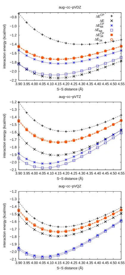
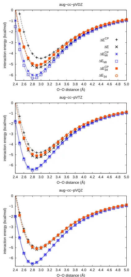
For the methane, water and hydrogen sulfide dimers geometry optimizations were car- ried out at the RI-MP2/aug-cc-pVDZ [97, 98] level of theory using the TURBOMOLE 5.10 program package [99] for fixed C-C, O-O and S-S distances, respectively. No symmetry constraints were imposed. Pictures of the optimized equilibrium structures are shown in Fig. 3.3. The interaction energies were calculated at RI-MP2 geome- tries at the CCSD(T), CCSD and MP2 [100, 101] levels of theory using the MOLPRO program package [102] and basis sets of augmented correlation-consistent double- through quadruple-ζ quality (aug-cc-pVXZ; X=D,T,Q) [67, 103]. Additional single point calculations on the helium dimer were performed with double and triple aug- mented correlation-consistent basis sets of double- through sextuple-ζ quality (y-aug- cc-pVXZ; y=s,d,t; X=D,T,Q,5,6) [69]. The frozen-core approximation was applied in all calculations except for He

.

In order to evaluate the correlation contribution to the interaction energies according to Eq. 3.8 the implementation of the incremental scheme [104] was used to get the necessary two-body increments. In order to obtain the proper fragments the domain size parameter (dsp, refer to Eq. 2.65) was set to the number of correlated orbitals on one fragment.

The convergence of the HF interaction energies was analyzed with basis sets of aug-cc-

pVDZ through aug-cc-pV6Z quality at the equilibrium structures for the methane, hy-

drogen sulfide and water dimers, see Fig. 3.4. The largest change in the CP-corrected interaction energy of the quadruple-ζ basis set with respect to the sextuple-ζ basis set is only -0.01 kcal/mol. Since the differences due to the correlation contributions dis- cussed in this work are much larger, the CP-corrected HF energies of the quadruple-ζ basis sets have been used as an approximation for the HF contributions to the extrapo- lated energies according to Eq. 3.3.

The discussion is limited to the CCSD(T) results in the following. The findings for

the CCSD and MP2 methods show a similar behavior with respect to the accuracy and

applicability of the procedure discussed. Therefore the conclusions presented below

are also valid at CCSD and MP2 level of theory. The CCSD and MP2 outcomes are

given in the Appendix A.

0.30 0.35 0.40 0.45 0.50

2 3 4 5 6

interaction energy (kcal/mol)

X (CH₄)₂

∆E^CP_HF

∆E_HF

-0.40 -0.35 -0.30 -0.25 -0.20 -0.15 -0.10 -0.05 0.00

2 3 4 5 6

interaction energy (kcal/mol)

X (H₂S)₂

∆E^CP_HF

∆E_HF

-3.90 -3.85 -3.80 -3.75 -3.70 -3.65 -3.60 -3.55 -3.50

2 3 4 5 6

interaction energy (kcal/mol)

X (H₂O)₂

∆E^CP_HF

∆E_HF

Figure 3.4: Counterpoise corrected and uncorrected HF interaction energy of the

methane, hydrogen sulfide and water dimer at equilibrium distance with

respect to the aug-cc-pVXZ (X=D,T,Q,5,6) basis set series.