Optimal discrete hedging of American options using an integrated approach to options with complex embedded decisions

Optimal discrete hedging of American options using an integrated approach to options with complex embedded

decisions

J. Gerer

, G. Dorfleitner

a

University of Regensburg, Department of Finance, 93040 Regensburg, Germany

Abstract

In order to solve the problem of optimal discrete hedging of American options, this pa- per utilizes an integrated approach in which the writer’s decisions (including hedging decisions) and the holder’s decisions are treated on equal footing. From basic prin- ciples expressed in the language of acceptance sets we derive a general pricing and hedging formula and apply it to American options. The result combines the important aspects of the problem into one price. It finds the optimal compromise between risk reduction and transaction costs, i.e. optimally placed rebalancing times. Moreover, it accounts for the interplay between the early exercise and hedging decisions.

We then perform a numerical calculation to compare the price of an agent who has exponential preferences and uses our method of optimal hedging against a delta hedger. The results show that the optimal hedging strategy is influenced by the early exercise boundary and that the worst case holder behavior for a sub-optimal hedger significantly deviates from the classical Black-Scholes exercise boundary.

Keywords: Transaction costs, early exercise, discrete hedging, American option, embedded decisions, good-deal bounds

JEL classification codes: G13, C61

Email addresses: ssrn@gerer.name (J. Gerer), gregor.dorfleitner@ur.de (G. Dorfleitner)

1. Introduction

Whenever an option writer hedges an option, their net payoff is given by the option’s premium minus the tracking error of the hedging activity. For European options and in a complete market, there is one hedging strategy that will turn the random future tracking error into a constant known at inception, rendering the pricing problem trivial. In reality, markets are neither complete nor friction-less and there are options and other claims whose payoff can be modified by the holder. Thus, in practice, the tracking error is random and can depend on a time-continuum of decisions by both the writer (deciding whether to change the current hedging position) and the holder (e.g. in the case of the American option, deciding whether to exercise or not).

While both aspects enjoy extensive treatment in scientific publications, most con- tributions only look at one aspect in isolation from the other, i.e. they focus either on realistic (discrete) hedging or on exercise features. The common ad-hoc approach to decisions embedded in option contracts is stretched over its limit, when applied to a complex combination of decisions by both counterparties.

This issue concerns, among other fields, the literature on realistically hedging of American options, which despite its practical relevance comprises only a handful of contributions. These contributions provide important groundwork, and satisfy many requirements that are in our view desirable for a solution of the problem. This paper’s aim is to improve on existing work by combining all these requirements. Table 1 contains the requirements numbered from one to eight in the column headers and provides an overview of the requirements satisfied by each contribution.

American exercise

(1)

W orst-case holder

strategy (2)

No restriction

of hedgin

g times (3)

T ransac tion

costs (4)

W eighin g of

risk/cost (5)

Not only

su p er-hedging (6)

Risk

&

costs influence

price (7)

Time consistency

(8)

Chalasani and Jha (2001) 3 3 3 3 3

Bouchard and Temam (2005) 3 3 3 3 3

Coleman et al. (2007) 3 3

Roux and Zastawniak (2008) 3 3 3 3 3

De Vallière et al. (2008) 3 3 3 3 3

Constantinides and Zariphopoulou (2001)

3 3 3 3 3 3

Constantinides and Perrakis (2007)

3 3 3 3 3 3 3 n.a.

Ahn and Wilmott (2009) n.a. 3

Gobet and Landon (2014) n.a. 3 3

Table 1: Relevant literature

Due to the limited number of contributions we also include two notable, newer

contributions on optimal hedging of European options, that therefore violate require- ment 1.

Contributions failing the second requirement assume some externally given exer- cise strategy of the holder. As an example take Constantinides and Zariphopoulou (2001), who state that “[the holder’s exercise time is given by some predetermined stopping time τ, which] may be the optimal exercise time [...] in the absence of transaction costs”, or Coleman et al. (2007) claiming that “[t]he holder will choose an exercise strategy to maximize the option value to him; hedging decisions of the writer are irrelevant to his exercise decision.” This view neglects the existence of a possible exercise strategy of the holder which is more expensive to hedge and which would thus lead to too low selling prices and insufficient insurance against all possible holder behaviors.

The third requirement is violated if rehedging times are somehow restricted by an external mechanism e.g. by a predetermined number of hedges, or if rebalancing is only allowed after some risk measure exceeds a certain threshold (e.g. as in Ahn and Wilmott, 2009). Such a restriction is always sub-optimal, because it ignores the fact that at any given point of time, rebalancing is optimal if and only if the reduction in risk does outweigh the cost associated with rebalancing. This kind of sub-optimality implies unrealistic behavior: if a trade leads to a more favorable hedging position now, why should any past consideration stop the hedger from executing it?

These considerations also originate the need to include transaction costs (require- ment 4) — be it traditional transaction fees, spreads or opportunity costs. Without transaction costs, the optimal hedging strategy always consists of quasi-continuous rebalancing, i.e. rebalancing to the optimal hedging position as fast as practically possible, which is simply unrealistic.

As mentioned above, deriving an optimal hedging strategy means weighing risk against transaction costs (requirement 5).

Requirement 6 might seem superfluous as it could be argued that the derivation of a super-hedging price actually satisfies requirement 5. However, the underlying risk-measure is too risk-averse to be realistic. Option writers do accept the risk of hedging losses, hence requirement 6.

Requirement 7 demands the remaining risk and transaction costs to actually con- tribute to the final option price. This requirement is for example missed by Gobet and Landon (2014). They minimize the product of the number of hedges and the quadratic variance of the hedging error, two quantities undoubtedly influencing the bottom line of a real-world hedging activity. However, their combination into a prod- uct is completely arbitrary and does not translate into a consistent option price, for there will always exist hedging strategies that do not optimize the above product and still lead to a lower selling price.

Time consistency (requirement 8), which is neglected in many contributions, is an important property, especially in the context of pricing options with complex decisions. Results obtained by time-inconsistent methods will either assume sub- optimal future choices or do not give the optimal solution from today’s perspective (see Gerer and Dorfleitner, 2016, for more details on the relation of decisions and time consistency in option pricing).

The article of Constantinides and Perrakis (2007) actually satisfies nearly all of our requirements, yet their contribution consists of the derivation of stochastic bounds on option prices for utility maximizing agents and thus has a different focus.

The isolated treatment of the two decisions by the holder and the writer com-

pletely ignores one of the core aspects of realistically hedged options, namely their

interplay. Questions about the possibility of a holder’s strategy that explicitly exploit

e.g. a fixed number of hedges by the writer or makes the original hedging strategy inhibitingly expensive due to transactions costs are not even considered.

This paper solves the problem of realistically pricing and hedging an American option. It is based on the insight that a realistic hedging theory is always a theory of hedging with transaction costs: it is not the physical impossibility of continuous trading that needs to be addressed.

Instead, we allow continuous trading (in the limit), but acknowledge that there is some kind of cost associated with each trade.

This cost is weighed against the remaining hedging risk. Expressing both risk and transaction costs monetarily, gives rise to an optimization problem whose solution is a finite number of optimally placed hedging trades and a consistent option price.

Our approach is motivated by the understanding of a “price” as an intrinsically one-dimensional quantity, which does not leave much conceptual freedom. The results from Gerer and Dorfleitner (2016) imply, that under mild assumptions, the decisions can be formally eliminated from the problem in a consequent manner without the need to resort to external concepts and without any further motivating argument.

Our analysis differs from others in that we seek to calculate the agent’s indifference or reservation price in an uncompromising fashion.

In Section 2, we summarize the formalism and results from Gerer and Dorfleitner (2016) used in this paper. In Section 3, a general duality between pricing functions and acceptance sets for payoffs with decisions is applied to derive a general pricing and hedging principle for options with decision by both parties. Section 4 specializes this principle to a formula for American options, which is then numerically solved in Section 5. Conclusions are given in Section 6.

2. Theoretical fundament

The theory is formulated from the perspective of a single market participant, that we will refer to as agent, engaging in financial activities and entering contracts with other agents, collectively called her counterparty.

All possible evolutions of the world, their physical probabilities and the time-dependence of information are described by a filtered probability space (Ω, F, {F _t } _t∈T , P ), where all points of time are given by the totally ordered set T .

Let L ^G _t represent all F _t -measurable random variables into the set G ⊆ R . We will use the abbreviations L t ≡ L

_t , L

_t ≡ L

_t , L

_t ≡ L

_t and L

_t ≡ L

_t , and employ the convention ∞−∞ = ∞ on R . Define also the set of positive t-premiums V t ≡ n

x ∈ L

_t

0

< x o .

We assume decisions happen at predetermined times, T d ⊆ T . As we will see later, this does not prevent us from describing more complex decision for which the point of time can also be chosen by the agent, like options with American exercise.

At each point of time t ∈ T d there can be exactly one decision by either the agent or the counterparty. This poses no limitation, as instantaneous decisions by the same agent can be merged into a tuple of decisions and it ensures that there is always a well-defined order between decisions by different agents, even if the physical time between them can be infinitesimally short. Decisions to be made by the agent happen at times T a and decisions by the counterparty at times T c ≡ T d \ T a .

1

With today’s trend to sub-millisecond order execution, continuous hedging could be approxi-

mated sufficiently if there were no transaction costs.

The decision behavior of the agents will be modeled by decision procedures, de- scribing how the choices for a subset of decisions depend on the world state. The set of decision procedures for decisions at times T ⊆ T d is abbreviated by Φ

and defined as the set of stochastic processes whose values at time t are elements of D _t :

Φ

≡ (

ϕ : T × Ω → [

t∈T

D t

ϕ t : Ω → D t , for all t ∈ T )

(1) D t contains all possible choices at time t. We will use the abbreviation Φ ≡ Φ

.

The payoff of an option with embedded decisions is described by specifying the cu- mulative discounted cash-flow to be received by the agent for any possible combination of choices and world states:

Definition 2.1 (Payoffs). Define X

^t as the set of F t -measurable payoffs that only depend on decisions made at times T ⊆ T :

X

^t ≡ n

f : Φ → L

_t

f (ψ) = ^B f (ϕ), if B ∈ F t and ψ t

= B ϕ t for all t ∈ T ∩ T d

o

Putting a set B ∈ F

above a comparison operator means conditionally almost surely equal: x = ^B y ⇔ P ({x = y}|B) = 1, with {x = y} ≡ {ω ∈ Ω | x(ω) = y(ω)}.

We will use the abbreviations X

≡ X

and X ≡ X

.

Remark 1. If a random variable x ∈ L

is used in the context of payoffs, it is understood as the corresponding constant payoff given by ψ 7→ x, which is an element of X

, and vice versa.

If not stated differently, all operators, relations and also suprema/infima used on payoffs are the pointwise versions of their L

, P -almost sure, variants: f Rg ⇔ ∀ϕ ∈ Φ : f (ϕ)

R g(ϕ)

Furthermore, we provide an operation to produce the effective payoff, that results if an agent or counterparty follows a decision procedure for a certain subset of decisions.

These decisions can be considered fixed and the effective payoff does not depend on them anymore:

Definition 2.2 (Effective payoff). For any payoff f ∈ X and decision procedure ϕ ∈ Φ

define the effective payoff, f

ϕ

∈ X

by f

ϕ

(ψ) ≡ f (ϕ 1

+ ψ 1

), for all ψ ∈ Φ.

The framework aims to provide the tools to build and analyze pricing theories for options with decisions. This is achieved by providing a minimal characterization of acceptance sets and pricing functions, proving their equivalence, and thus making these concepts usable interchangeably.

A t-acceptance set contains the agent’s acceptable opportunities at time t, i.e.

payoffs without decisions before time t that she accepts as zero-cost investments. We require the following property to ensure that an acceptance set can serve as modeling tool for pricing theories:

Definition 2.3 (Proper acceptance sets). A t-acceptance set A is called proper if it is t-compatible (see below) and A =

f ∈ X

{f + x | x ∈ V _t } ⊆ A .

Definition 2.4 (t-compatibility). A non empty set X is t-compatible, if for all {x n } ⊆ X and mutually disjoint {B n } ⊆ F t with P ( S

n B _n ) = 1 it holds P

n x _n 1 B

∈

X , where 1 B

is the indicator function of the set B _n .

Remark 2. In this framework, the result of a pricing function is understood as the highest premium the agent would accept to pay for entering the contract, or her bid price. If a contract’s ask price is wanted, it can be calculated by the negative of the bid price of the reversed contract.

A t-pricing function is any function π : X

→ L

_t .

Remark 3. For a general option f ∈ X — possibly including decisions before t — and a t-pricing function π, we use π(f ) to denote ϕ 7→ π

f ϕ

, which is a payoff in the sense of Definition 2.1.

For pricing functions, the property corresponding to properness is cash invariance.

Definition 2.5 (Cash invariance). A t-pricing function π is called cash invariant if for any payoff f ∈ X and payoff g ∈ X

^t with no present or future decision and g > −∞, it holds π(f + g) = π(f ) + g.

We will also use the term normalized pricing function:

Definition 2.6 (Normalized pricing function). A pricing function π is called nor- malized, if π(0) = 0. Every pricing function π with |π(0)| < ∞ has a normalized version x 7→ π(x) − π(0).

As proved in Gerer and Dorfleitner (2016, Theorem 3.1) there exists a one-to-one correspondence between the set of cash invariant t-pricing functions and the set of proper t-acceptance sets. The duality operations are given in the following definition and correctly replicate the description of pricing functions in Remark 2:

Definition 2.7 (Duality operations). For any t-acceptance set A define its dual t- pricing function P [A] by P [A](f ) ≡ sup

x ∈ L

_t

f − x ∈ A for all f ∈ X

.

For any t-pricing function π define its dual t-acceptance set A[π] ≡ f ∈ X

0 ≤ π(f ) .

This duality enables us to develop our pricing theory for options with decisions in terms of the more directly accessible language of acceptance. Specifically, we will use conservative acceptance, which is employed implicitly in most of the option pricing literature. For a given t-acceptance set A and a set of admissible decision procedures S, A

and A

represent the conservative acceptance sets for decisions by the counterparty or the agent, respectively. A

includes an option if and only if for every possible decision procedure by the counterparty the resulting effective option is acceptable:

A

≡

f ∈ X

∀ϕ ∈ S : f ϕ

∈ A (2)

It is important to understand, that this presumes nothing about the counterparty’s actual behavior. For her own decisions, A

contains an option if and only if there always is at least one decision procedure the agent could follow to make the effective option almost acceptable, as indicated by the +x:

A

≡

f ∈ X

∀x ∈ V t , ∃ϕ ∈ S : f ϕ

+ x ∈ A (3)

2

The supremum is to be understood as the essential supremum, i.e. the supremum in the almost sure sense.

3

See Gerer and Dorfleitner (2016, Example 4.2) for why this definition needs a more complicated

form than Eq. (2)

In order to talk about acceptance sets and pricing functions at different times, we introduce acceptance families as time indexed families of proper acceptance sets {A t } t written as A

and pricing families, as time indexed families of cash invariant pricing functions written as π

.

An especially important property of such families is time consistency (require- ment 8 in Table 1). By Theorem C.6, the following definitions are equivalent:

Definition 2.8 (Time consistency). A proper acceptance family A

with a normalized dual π

is called time consistent if f ∈ A t ⇐⇒ π s (f ) ∈ A t , for all s ≥ t.

A normalized pricing family π

is called time consistent if for all s ≥ t and f ∈ X:

π t (π s (f )) = π t (f ).

3. Optimal hedging — the general formula

We will treat the hedging activity as decisions within our theory of options with decisions. Between rehedges there can be further decisions for both the agent and its counterparty.

This approach will produce the pricing function for the hedging agent as well as the optimal hedging ratios, i.e. optimally placed rehedgings, without the need to formulate an exogenous optimization problem. Instead these results are direct consequences of the construction and imposed properties of the acceptance set and their relation to pricing functions.

We impose no practical limitation on the number of rehedgings the agent can perform. For formal reasons, we approximate the set of hedging decisions using a finite, increasing sequence (τ _i ) _i≤n , where the hedging position is closed on the last date τ _n .

Remark 4. While this introduces a dependency of the results on the particular choice of this sequence, the time intervals can be made smaller than any physical time scale of our world and thus its practical influence eliminated. Numerical calculations typically will be feasible only for much larger intervals.

The actually number of performed rehedgings will usually be smaller than n, as at each time τ i the agent can decide not to rebalance her hedging portfolio.

The discounted price processes of the assets available for hedging are modeled by an N -dimensional adapted process X = (X _t ) _t with finite components. A hedging decision consists of choosing the amount of shares to hold from each asset, which we will model using N-dimensional vectors, i.e. D _τ

⊆ R ^N for all i ≤ n.

Given a decision procedure ϕ ∈ Φ, the future cash-flow of a hedging activity started with an initial position ϕ τ

at a time t ∈ (τ _i−1 , τ i ] is given by

H t (ϕ) ≡

n+1

X

j≥i

ϕ τ

· X τ

− X

_,t}

− C j (ϕ). (4)

The · marks scalar product between two vectors. The first term calculates the gains from market price movements, and C _j (ϕ) stands for the finite, F _τ

-measurable trans- action costs associated with changing the portfolio from ϕ _τ

to ϕ _τ

at time τ _j . C _n+1 corresponds to the special case of liquidating the last position ϕ _τ

at τ _n+1 . It is easy to see that H t depends on decisions at time τ _i−1 and later, i.e. H t ∈ X

i−1

.

In order to derive the general pricing function of the hedging agent for options

with decisions, we employ the method of Gerer and Dorfleitner (2016, Section 4.3) to

derive the super-replication price for continuous trading. We start with the agent’s

internal acceptance family, A

, containing payoffs or zero-cost investments she accepts

“as is”, i.e. payoffs that cannot be modified by her beyond the decisions contained in the payoff, especially not be hedged against. A

needs to capture the agent’s risk aversion, business model and regulatory requirements. In this section we treat it as given, for it is completely independent from the aspect of hedging; a separation of concerns made possible by the development of the proposed framework.

Next, this acceptance family is transformed into the agent’s external acceptance family, B

, by subtraction of any modifications, which are not part of the original contract specifications. In the current setting this means subtracting the proceeds of her hedging activity:

B t (ϕ) ≡ n f − H _t

ϕ

f ∈ A t

o (5) B t depends on the decision procedure ϕ, because H t depends on past decisions, more specifically on the most recent hedging decision. Making this dependency ex- plicit ensures, that B t (ϕ) itself contains only options with no past decisions.

Eq. (5) can also be read in the following way: The agent accepts a contract with another party, if and only if, she internally accepts the contract’s payoff plus the result of her hedging activity.

Through the duality we know that these acceptance sets uniquely define the hedg- ing agent’s prices – denoted by η

, which can be calculated using the duality operation from Definition 2.7:

η t (f )(ϕ) ≡ P[B t (ϕ)](f )(ϕ) (6)

for any option with decisions f ∈ X and decision procedure ϕ ∈ Φ.

Of course, η

can also be expressed using A

’s dual pricing family π

= P [A

]:

Lemma 3.1. η t (f ) = π t (f + H t ) for all t and f ∈ X.

Proof. See Appendix B.1.

This is in agreement with the expected result that the price of an option is given by the internal price of the hedged option.

Remark 5 (Normalization). The above construction of η

will in general not yield normalized pricing functions, i.e. the price of the zero payoff is different from zero:

η t (0) = π t (H t ) 6= 0. Depending on the specific nature of A

and π

, it is possible that the agent assigns a positive net present value to the proceeds of the trading activity H i , i.e. π τ

(H i ) ≥ 0. This can happen for example, if π t (X s ) > X t (for s > t), i.e. buying or selling the market assets represents an acceptable or even arbitrage opportunity.

If the market is arbitrage free, or the agent’s transaction costs destroy any accept- able or arbitrage opportunity, then π τ

(H τ

)(ϕ) is zero, if ϕ τ

= 0 and even negative for ϕ τ

6= 0, due to the unavoidable costs for closing the current position eventually.

Economically meaningful prices are obtained from the normalized version:

f 7→ η t (f ) − η t (0)

This calibration ensures that the price of any sure payoff equals the payoff itself

(η t (g) = g if g ∈ L

_t , which follows from cash invariance), and it is plausible with the

two cases described above: If the agent would pay a positive amount η t (0) > 0 for the

situation he already is in, normalization decreases all bid prices by that amount, which

could be interpreted as compensation for giving up the current favorable position upon

entering the new contract. In other words, normalization erases the additional value

η t (f) assigns to the possibility of trading in the market, which the agent can also do without f and whose value is thus given by η t (0).

For an initial unfavorable position ϕ τ

6= 0, η t (0) ϕ

would be a negative number representing the negative of the cost associated with optimally closing that position.

In this case normalization would increase the agent’s naked bid price η _t (f ), because entering and optimally hedging f would spare her the cost of closing her current position.

In addition to the hedging decisions, we explicitly add times for general counter- party decisions, which will then be used for the early exercise decision in the next section. Between any two hedging times τ i and τ i+1 there is a decision of the coun- terparty located at s i :

τ i < s i < τ i+1

Furthermore, for each decision we need a set of admissible decision procedures, de- noted by R _i ⊆ Φ

and S _i ⊆ Φ

for all i ≤ n.

The general result needs the following axioms. The first assures that hedging de- cision cannot see in the future. The additional requirement of t-compatibility derives from the technical differences between conservative acceptance for the agent and the counterparty (cf. Theorems C.4 and C.5):

Axiom 1. For all i ≤ n, R _i contains only F t -adapted decision procedures and is τ _i -compatible (cf. Definition 2.4).

The second axiom specifies how decisions are treated. We use conservative accep- tance (as defined in Eqs. (2) and (3)) at the time of each particular decision. This, together with time consistency, will be enough to eliminate all future decisions from the pricing problem.

Axiom 2 (Conservative acceptance). A τ

= A

_τ

and A s

= A

_s

for all i ≤ n.

Feeding all this into our formalism yields the pricing formula for an optimally hedged option:

Theorem 3.2 (Optimal hedging). Let a A

be a time consistent internal acceptance family with a normalized dual pricing family π

and assume Axioms 1 and 2. At the end of the hedging activity, the price of an option f ∈ X can be calculated directly by

η τ

(f ) = π τ

(f ) − C n+1 , (7)

and earlier prices for i ≤ n can be calculated recursively:

η τ

(f) = sup

ϕ∈R

π τ

ψ∈S inf

π s

η τ

(f ) ϕ

ψ

+ ϕ τ

· X τ

− X τ

− C i ϕ

(8) Proof. See Appendix B.2.

For a hedging strategy a and decision procedure of the counterparty b, the net payoff of the whole hedging activity is given by the difference of the realized tracking error and the option’s upfront premium:

δ ≡ (f + H t ) a

b

− η t (f )

Conservative acceptance ensures, that for any decision procedure b and ∈ V _t there

exists a hedging strategy a such that δ + is acceptable.

4. Optimal hedging of American options

In this section we specialize the results from the previous section in order to price and hedge an American option from the perspective of the writer. The holder of an American option with discounted exercise value process g has the right to exercise it at any time t prior or equal to the expiration date T and receive the amount g t .

This exercise right gives rise to infinitely many decisions: At every instant the holder can decide to exercise or not to exercise. To model these decision we use the finite set of decision times {s i } introduced in the last section, with s n ≡ T . Following the reasoning from Remark 4 this implies no loss of generality. We define

D _s

≡ {1, 0}, where 1 stands for “exercise” and 0 for “do not exercise”, (9) for all i. The payoff of an American option that has not been exercised before time s _i is then for any ϕ ∈ Φ and ω ∈ Ω given by:

f i (ϕ) ≡ g t

with the stopping time t

(ω) = min{t ≥ s i | ϕ t (ω) = 1} (10) This definition shows the expected behavior, if the current decision is fixed using a constant decision procedure:

f i

s i 7→ 1

= g s

for exercise, and f i

s i 7→ 0

= f i+1 for continuation. (11) Basic theory of stochastic processes ascertains that f is measurable if g is progressively measurable and ϕ is adapted. And thus due to Corollary A.1 and f i ’s pointwise definition it is a payoff according to our Definition 2.1, or more precisely f i ∈ X

j=i

, as it only depends on decision at times {s _i , . . . , s _n }.

While we restrict the admissible hedging procedures through Axiom 1 from the last section, the only restriction placed on exercise procedures is their being adapted:

S i ≡ Φ

∩ {ϕ | ϕ is adapted to F}, for all i. (12) So far the optimizations in Theorem 3.2 have to be performed over random vari- ables making a direct numerical implementation infeasible. However, as they are limited to “current time” decisions, they can be simplified. We give sufficient (but not necessary) conditions under which the essential supremum over the set of proce- dures can be simplified to a pointwise supremum directly over the set of choices:

Lemma 4.1 (Countable present time decisions). If D _t or Ω is countable and S ≡ Φ

∩ {ϕ | ϕ is adapted to F}, then for every cash invariant t-pricing function π and f ∈ X it holds:

sup

ϕ∈S

π f ϕ

= sup

a∈D

π f t 7→ a

Proof. See Appendix B.3.

As the payoffs involved do not have any decisions besides the hedging and exercise

decisions, we can give a result that reduces the pricing problem to classical option

pricing theory for options without decisions. To make this explicit we will use A

and

π

to denote the restrictions of A

and π

to options without decisions. Formally, we

define A

≡ A

∩ X

and π

= P[A

]. Lemma C.1 proves the expected connection

between π

and π

.

Furthermore, we assume for all i that the agent’s hedging decision at τ i+1 hap- pens instantly after the exercise decision s i . Formally, these two times collapse for quantities that do not depend on the decision at s i , i.e.

g _s

= g _τ

, and π _s

(f ) = π _τ

(f ), if f ∈ X

,∞i . (13) Now we can derive the main result:

Theorem 4.2. Given X , C, A

, {R _i } and η

as in Theorem 3.2, {S _i }, f, A

and π

as defined above, we define p i as the ask price (cf. Remark 2) at time τ i of an optimally hedged American option:

p i ≡ −η τ

(−f i ), for all i ≤ n.

The price after expiration is given by

p n+1 = C n+1 , (14)

and earlier prices for i ≤ n can be calculated recursively:

p _i = inf

ϕ∈R

−π _τ

−max

g _τ

− η _τ

(0), p _i+1 ϕ

+ ϕ _τ

· X _τ

− X _τ

+C _i

ϕ (15) Proof. See Appendix B.4.

As expected, the writer chooses the most favorable hedge and it is most expensive for her if the holder exercises as soon as the payoff exceeds the price of the continued option.

The terms C n+1 and −η τ

(0) = −π _τ

(H i ) occurring above could be identified with the cost of optimally closing the current hedging position. As already discussed in Remark 5, they are non-negative in a market without acceptable opportunity and thus add to the payment of g τ

faced by the hedging option writer upon exercise by the holder.

Their appearance is a consequence of the fact that η

is not normalized (in gen- eral) and it can be trivially checked, that normalizing the result — i.e. calculating p i + η τ

(0) — would remove both terms, whilst introducing a similar term in the con- tinuation value. We did not state the normalized result, as it would complicate the recursive calculations, which are more naturally expressed in unnormalized values.

5. Numerical demonstration

In this section we produce numerical results from Theorem 4.2. We will use a simple market model consisting of a riskless money market account with interest rate r and a single stock whose discounted price process X

is a geometric Brownian motion with drift µ > r and volatility σ. Besides analytical tractability and intuitiveness, it reveals interesting features of the pricing and hedging problem. It should be noted that our hedging formula can be applied to any model for the price process X.

We are pricing an American put with strike K, i.e. a payoff f as defined in Eq. (10) with discounted exercise value written as g t (X t ) = X t − Ke

.

The transaction costs consist of a fixed component k

and a component propor- tional to the transaction value (with factor k

). Its discounted value is calculated as follows:

C i (ϕ) ≡ c i (ϕ τ

− ϕ τ

, X τ

) with c i (q, x) = e

k

1 q6=0 + k

x |q|

5.1. Selecting a pricing function

Before we can actually implement a numerical program, we need to devise the agent’s internal pricing family for options without decisions, π

Let us first state the requirements to be met by π

. There is, of course cash invariance (requirement I), the basic property imposed by our formalism, and time consistency (requirement II) upon which the results of the previous section rely.

In addition to these two requirements concerning π

directly, we place three further restrictions on the resulting external pricing family η

(cf. Lemma 3.1). To ensure con- sistency with existing results we require that without transaction costs and in the limit of infinitely many hedging times the well-known arbitrage-free prices, i.e. risk-neutral expectation values, are obtained for continuously replicable payoffs (requirement III).

As noted in Remark 5, η

is not normalized. Thus, η _t (0) = π _t (H _t ) can be negative due to transaction costs for closing the current position or positive, if trading in the market constitutes an acceptable opportunity for the agent. While these effects can be handled satisfactory by normalizing the result, normalization is only meaningful if

|η t (0)| < ∞, or informally stated, if the agent cannot extract infinite wealth from his trading activity (requirement IV).

Besides these theoretical requirements, for the purpose of this demonstration we need readily implementable, numerical algorithms (requirement V).

To satisfy requirement V we exclude all pricing functions or risk-measures whose calculation relies on Monte Carlo methods. We are aware of the existence of Monte Carlo methods suitable for American options, but extending and implementing them for our problem — while deemed possible — would go beyond the scope of this paper.

This excludes all candidates containing the value-at-risk and its variants or derivatives like the expected shortfall or conditional value-at-risk, most of which also violate requirement II, time consistency (cf. Cheridito and Stadje, 2009).

We use π

_t (f ) ≡ −1

γ ln E e

F t

, (16) for some positive degree of risk aversion γ. This function is the indifference price of the exponential utility function, also known as the negative of the conditional entropic risk measure and has gained much attention in the field of utility indifference pricing, among others.

For the remainder of this paper we use the pricing family η

as defined in Eq. (6) for an acceptance family A

satisfying Axiom 2 and A

∩ X

= A

π

with π

as defined above in Eq. (16). We also define the normalized pricing family η

:

η _t (f ) ≡ η t (f ) − η t (0), for all f ∈ X

It is well-known (see e.g. Cheridito and Kupper, 2009, Eq. 3.3) that π

is cash invariant (requirement I) and time consistent (requirement II). It also satisfies re- quirement V, because PDE discretization methods for the calculation of conditional expectations are widely-used and can be applied directly to solve Eq. (15) from The- orem 4.2.

We do not present a formal proof of requirement III for η

, but instead point out

two supporting facts. First, for continuous trading strategies without transaction

costs it has been shown that η

yields the risk-neutral expectation value (cf. Davis

et al., 1993, Theorem 1, or for a more recent presentation Becherer, 2003, Eq. 3.8, who

calls this elementary no-arbitrage consistency). Secondly, we confirmed by numerical

calculations that making the time between two rehedges short enough will result in

prices sufficiently close to the Black-Scholes price and optimal strategies coinciding with the Black-Scholes delta.

Again without a formal proof, requirement IV follows from another well-known result (see e.g. Henderson and Hobson, 2002, Eq. 2): In the case of continuous trading without transaction costs, it holds that η _t (0) < ∞ and the optimal strategy is given by:

Z _t (X _t ) ≡ µ − r γσ

X t

(17) Due to the monotonicity of the supremum in Theorem 3.2 and the monotonicity of π

, restricting to discrete strategies and introducing transaction costs results in even smaller prices.

5.2. Translating Theorem 4.2 into a computational procedure

In order to perform the hedging optimization numerically we only consider a finite number of different hedging positions, i.e. D _τ

finite for all i ≤ n. Then Lemma 4.1 and the Markov property of X

enable us to write Theorem 4.2 in a form suitable for numerical calculation. Using the ordinary functions z _i (h, X _τ

) ≡

−η _τ

(0)

τ _i−1 7→ h

for the price of the zero claim and v _i (h, X _τ

) ≡ max

g _τ

(X _τ

) + z i (h, X τ

), −η τ

(−f i )

τ i−1 7→ h for the price of the optimally hedged option, both with a current hedging position h, we get:

v _n+1 (h, x) = max

g _τ

(x), 0 + c _n+1 (h, x) z n+1 (h, x) = c n+1 (h, x)

Cont i (h, x, b, q) ≡ 1 γ ln E t

h

e ^γ ( ^b

)

X τ

= x i

+ q x + c i (h − q, x) q _τ

i

(h, x) ≡ arg min

q∈D

Cont i (h, x, v, q) (18)

v i (h, x) = max n

g τ

(x) + z i (h, x), Cont i (h, x, v, q

(h, x)) o

(19) z i (h, x) = min

q∈D

Cont i (h, x, z, q)

We are going to compare the price obtained under the optimal hedging strategy q

with classical delta hedging. Let d represent the ask price of an agent who rebalances daily to the optimal continuous, zero-transaction costs strategy given by the sum of the option’s Black-Scholes delta, ∆ t (x) = _∂x ^∂ BS t (x), and the utility optimizing strategy from Eq. (17), Z _t (x):

d _n+1 (h, x) = v _n+1 (h, x) (20)

d i (h, x) = max n

g τ

(x) + z i (h, x), Cont i (h, x, d, ∆

(x) + Z

(x)) o bτ _i c rounds down τ _i to the beginning of the most recent day.

Our numerical program written in C++ is a direct translation of the above equa- tions. The conditional expectations are calculated using a finite difference method with optimal spatial finite difference weights à la Ito and Toivanen (2009) and Crank- Nicolson time-stepping with Rannacher startup (Rannacher, 1984; Giles and Carter, 2006). The expectation values in Cont i (h, x, b, q) are calculated for all pairs (b, q) ∈ {v, z, d} × D τ

in parallel, achieving quasi-linear speedup on multi-core CPUs.

We will write normalized prices as v ≡ v − z and d ≡ d − z.

5.3. Numerical results

We now present the results of the calculation using the following specifications.

The American put has a strike price K = 100, volatility σ = 50% p.a., drift µ = 10% p.a., risk-free rate r = 5% p.a., where one year consists of 252 business days.

We assume very moderate transaction costs, with a fixed component of k

= 0.001 and proportional component of k

= 0.025%. The writer’s coefficient of constant absolute risk aversion is γ = 0.001.

We use 8 hedging and exercise decision times per day, i.e. τ i+1 −τ i =

/

day. There are 150 allowed hedging positions, D τ

= {0, δ, 2δ, . . . , 5} with δ =

/

≈ 0.0336.

Using a higher numbers of daily decisions and possible hedging positions does not significantly change the calculated values.

The results comprise three aspects: the writer behavior, the holder behavior and the option price.

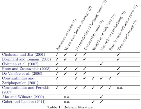
The writer’s optimal hedging position is given by q

_t (x, h) from Eq. (18) and de- pends on current stock price x and hedging position h. Figure 1 plots two examples for fixed values of h. Instantly after rebalancing to this optimal position, h

≡ q

_t (x, h), the current stock price x will lie in one of possibly several plateaus where x 7→ q

_t (x, h

) is constant with value h

. As soon as the stock price leaves this plateau, it is again optimal to rebalance.

The information contained in q _t

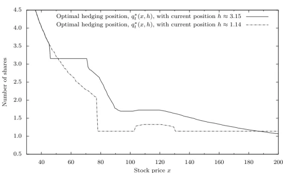
can be completely described by two corridors, the no-trading and the rebalancing corridor. They are depicted in Figure 2 for two different times t and have the following interpretation: it is optimal to rebalance to the nearest point of the rebalancing corridor, but only if the stock price leaves the no- trading corridor. The spikes visible in Figure 2 in both corridors occur in the vicinity of the optimal exercise boundary of the holder. An effect, of course only revealed by solving the full optimization problem.

Based on experiments with different values of k

and k

, we make the following numerical observations. The rebalancing corridor is always fully contained within the no-trading corridor, its width is monotonically increasing in k

, the proportional component of the transaction costs, and it collapses for k

= 0. The space between the two corridors exhibits an analogous relationship with k

, the fixed component. The delta hedging position lies within the no-trading corridor and for stock prices above the exercise boundary also within the rebalancing corridor. Without transaction costs both corridors collapse to the delta hedging strategy.

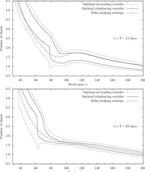
The exercise behavior of the holder is characterized by the exercise boundary, which separates the continuation regions from the their complement, the exercise regions. With conservative acceptance the writer is insured against the worst possible or pessimal exercise strategy. The corresponding continuation regions consist of states where the maximum in Eq. (19) or Eq. (20) equals the continuation value.

Figure 3 shows the holder’s pessimal exercise boundaries against different writers.

Against the optimal hedger the continuation region is only slightly larger than in the

Black-Scholes case. The most striking finding is that the holder could in fact harm the

delta hedger. The boundary against the delta hedger clearly exhibits a daily recurring

pattern lining up with her daily rebalancings. As expected, the continuation region

is much larger than in the optimal case, which can be explained by the fact that con-

tinuing the claim means more hedging costs for the (sub-optimal) delta hedger. This

holds true as long as the delta hedger actually rebalances and thus incurs transaction

costs. If the delta hedger’s current position equals the next delta hedging position,

there are no transactions costs and thus at these points (also marked in Figure 3) the

extended continuation region stops.

This shows that for a delta hedger the common assumption of a Black-Scholes exercise boundary will result in an underestimation of risk caused by the interplay of American exercise feature, discrete hedging and transaction costs.

Holder and writer behavior are by-products of the main result: the price. Figures 4 and 5 provide two different perspectives on the put’s normalized ask prices of an optimally hedging writer, v, and a delta hedging writer, d. Figure 4 shows how the absolute difference v − d depends on the current hedging position for fixed stock prices. As is expected, once it is optimal to rebalance, the additional transaction costs of both optimal and delta hedging will be equal, making the difference between the two independent of the current hedging position.

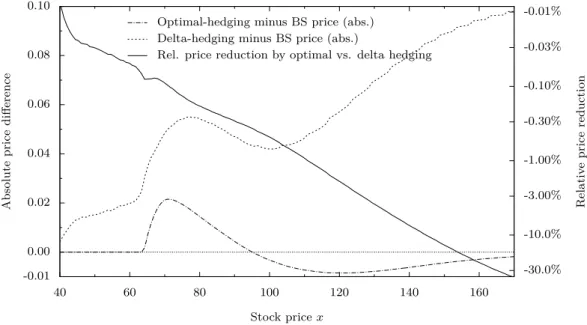
For a fixed current hedging position and varying stock prices the difference between both prices and the Black-Scholes price are reflected in Figure 5. It also contains the relative price reduction to be achieved by optimal hedging, calculated as ^d / v − 1.

Both figures demonstrate that the writer can always offer a more competitive price or make a sure profit by optimal hedging instead of delta hedging. This profit increases with decreasing moneyness. For example, 63 days before expiration at a stock price of 145.3, the optimal-hedging price is v ≈ 0.787, which is 10.3% lower than the delta-hedging price.

Last, reducing the risk aversion increases both the optimal-hedging and the delta- hedging price. However, the effect on the delta-hedging price is weaker and conse- quently, the profit from optimal hedging will be larger for a less risk-averse agent. In the above example, if we change γ to γ/2 = 0.0005, v will be 17.3% lower than d.

6. Conclusion

Applying the methods of Gerer and Dorfleitner (2016) to the problem of hedging options with decisions allows us to derive a general hedging principle in a rigorous but straight forward manner, starting from a small set of clearly stated assumptions. This principle is then further specialized to a formula for realistically hedging American options; a formula that is not conjectured, but formally derived and proved in non- preexisting fashion.

To demonstrate how to turn this completely model-independent formula into ac- tual numbers, we fix a market model, a pricing function and transaction costs and perform numerical calculations. The results of these numerical experiments show that when compared to the delta hedger, the optimal hedger can offer a significantly bet- ter price or make a sure profit. Further, they reveal that indeed there is a complex interaction between hedging decisions and the early exercise decisions.

In addition to the conceptual and theoretical advantages demonstrated by our holistic approach to decisions embedded in option contracts, these results prove the usefulness of our method in realistic applications.

We leave it to further research to apply our methods more realistic models than

the above example and to overcome the challenge of a numerical implementation of

our results for these models.

0.5 1.0 1.5 2.0 2.5 3.0 3.5 4.0 4.5

40 60 80 100 120 140 160 180 200

Num b er of shares

Stock price x

Optimal hedging position, q

(x, h), with current position h ≈ 3.15 Optimal hedging position, q

(x, h), with current position h ≈ 1.14

Figure 1: Optimal hedging position at time t = T − 11 days, q

(x, h), for different stock

prices x and two different current positions h. It is optimal not to rebalance if

the stock prices stay in regions with q

(x, h) = h.

0.5 1.0 1.5 2.0 2.5 3.0 3.5 4.0 4.5

40 60 80 100 120 140 160 180 200

t = T − 11 days

Num b er of shares

Stock price x

Optimal no-trading corridor Optimal rebalancing corridor Delta hedging strategy

0.5 1.0 1.5 2.0 2.5 3.0 3.5 4.0 4.5

40 60 80 100 120 140 160 180 200

t = T − 63 days

Num b er of shares

Stock price x

Optimal no-trading corridor Optimal rebalancing corridor Delta hedging strategy

Figure 2: The two graphs consolidate the optimal hedging behavior at two different times.

Only when the stock price leaves the no-trading corridor, it is optimal to re-

balance. The new optimal position is then given by the nearest point of the

rebalancing corridor. For comparison the delta hedging strategy, ∆

(x) + Z

(x),

is also shown.

40 50 60 70 80 90 100

0 5

10 15

20 25

30 35

(continuation region)

(exercise region)

(cont. r.)

Sto c k price x

Time to expiration, T − t, in days Pessimal exercise boundary against optimal hedger Pessimal exercise boundary against delta hedger Stock prices where no delta rebalancing is required Black-Scholes exercise boundary

Figure 3: Worst-case exercise behavior of the holder against optimal and delta hedg- ing writer with hedging position h ≈ 3.02, described by boundaries separat- ing exercise and continuation regions. We marked stock prices x that satisfy

∆

(x) + Z

(x) = h, i.e. where the delta hedger does not need to rehedge (cf.

Section 5.3). For comparison the Black-Scholes exercise boundary is also shown.

-0.09 -0.08 -0.07 -0.06 -0.05 -0.04 -0.03 -0.02 -0.01 0.00

0 1 2 3 4 5

Optimal-hedging − Delta-hedging price

Current hedging position

x

x

x

x

x

x

x

x

x

x

Figure 4: Price reduction achieved by optimal hedging compared to delta hedging, calcu-

lated at t = T − 63 days. Each line corresponds to a fixed stock price x and

varying current hedging positions.

-0.01 0.00 0.02 0.04 0.06 0.08 0.10

40 60 80 100 120 140 160

-30.0%

-10.0%

-3.00%

-1.00%

-0.30%

-0.10%

-0.03%

-0.01%

Absolute price difference Relativ e price reduction

Stock price x

Optimal-hedging minus BS price (abs.) Delta-hedging minus BS price (abs.)

Rel. price reduction by optimal vs. delta hedging

Figure 5: Comparison of normalized optimal-hedging, delta-hedging and Black-Scholes

price at time t = T −63 days with current hedging position h ≈ 4.83 for different

stock prices x.

Appendices

A. Pointwise defined payoffs

Corollary A.1. Given a function g : Ω × R

→ R and a sequence of times (τ i ) i∈

, define f :

f (ϕ)(ω) = g ω, (ϕ _τ

(ω)) _i∈

, for all ϕ ∈ Φ and ω ∈ Ω (21)

If f (ϕ) is F

-measurable for all ϕ ∈ Φ, then f ∈ X

N

.

Proof. As in Definition 2.1, we assume some set B ∈ F

and two decision procedures with ψ τ

= B ϕ τ

for all i. As a direct consequence of Eq. (21) we have T

i∈N {ϕ τ

= ψ τ

} ⊆ {f (ϕ) = f (ψ)} and applying basic set operations yields:

B \ {f (ϕ) = f (ψ)} ⊆ B \ \

i∈

{ϕ τ

= ψ τ

} = [

i∈

(B \ {ϕ τ

= ψ τ

}) From monotonicity and sub-additivity of the probability measure we follow:

P (B \ {f (ϕ) = f (ψ)}) ≤ X

i∈N

P (B \ {ϕ τ

= ψ τ

})

Due to P ({ϕ _τ

= ψ _τ

}|B) = 1 for all i (by assumption) and Corollary C.7.1 both sides of this inequality are zero and thus by the same Corollary P ({f (ϕ) = f (ψ)}|B) = 1.

B. Proofs

B.1. Proof of Lemma 3.1

Proof. Take any ϕ ∈ Φ and show:

P [B t (ϕ)](f)(ϕ) = sup n

x ∈ L

_t f

ϕ

− x ∈ B t (ϕ) o

= sup n

x ∈ L

_t

(f + H _i ) ϕ

− x ∈ A _t o

= π _t (f + H _i )(ϕ) The first and third equation use the definition of P[A] (Definition 2.7). The second uses the definition of B t (Eq. (5)).

B.2. Proof of Theorem 3.2

Proof. To prove Eq. (7), we start with Lemma 3.1 and apply cash invariance (Defini- tion 2.5, applicable due to H τ

= −C n+1 ∈ X

^τ

n}

).

To prove Eq. (8), we define ∆ ^b _a ≡ H a − H b . By H’s definition in Eq. (4) and Axiom 1 we can infer for any τ i < t ≤ τ i+1 and ϕ ∈ Φ:

∆ ^t _τ

i

(ϕ) = ϕ _τ

· (X _t − X _τ

) − C _i (ϕ) ∈ L _t and thus ∆ ^t _τ

i

∈ X

,τ

(22)