NBER WORKING PAPER SERIES
THE PERSISTENCE AND HETEROGENEITY OF HEALTH AMONG OLDER AMERICANS Florian Heiss
Steven F. Venti David A. Wise Working Paper 20306
http://www.nber.org/papers/w20306
NATIONAL BUREAU OF ECONOMIC RESEARCH 1050 Massachusetts Avenue
Cambridge, MA 02138 July 2014
Funding for this project was provided by the National Institute on Aging grants P01-AG005842 and P30-AG012810 to the National Bureau of Economic Research. The views expressed herein are those of the author(s) and do not necessarily reflect the views of the National Institute on Aging, the National Institutes of Health, or the National Bureau of Economic Research. The views expressed herein are those of the authors and do not necessarily reflect the views of the National Bureau of Economic Research.
NBER working papers are circulated for discussion and comment purposes. They have not been peer- reviewed or been subject to the review by the NBER Board of Directors that accompanies official NBER publications.
© 2014 by Florian Heiss, Steven F. Venti, and David A. Wise. All rights reserved. Short sections of text, not to exceed two paragraphs, may be quoted without explicit permission provided that full credit,
The Persistence and Heterogeneity of Health among Older Americans Florian Heiss, Steven F. Venti, and David A. Wise
NBER Working Paper No. 20306 July 2014
JEL No. I10,I19,J14
ABSTRACT
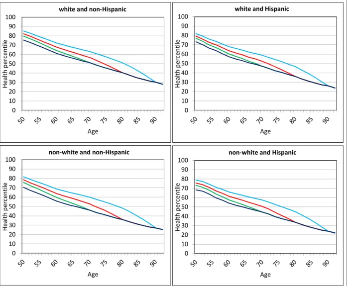
We consider how age-health profiles differ by demographic characteristics such as education, race, and ethnicity. A key feature of the analysis is the joint estimation of health and mortality to correctfor the effect of mortality selection on observed age-health profiles. The model also allows for heterogeneity in individual health at a point in time and the persistence of the unobserved component of health over time. The observed component of health is based on a multidimensional index based on 27 indicators of health. Most of the key results are shown by simulations that illustrate the range of issues that can be addressed using the model. Differences in health by education and racial-ethnic group at age 50 persist throughout the remainder of life. Based on observed profiles, the health of whites is about 8 percentile points greater than the health of blacks at age 50 but by age 90 the gap is only 5 percentile points. However, when corrected for mortality selection, the health of blacks is actually declining more rapidly with age than the health of whites; the true gap widens with age. We also find that much of the difference in age-health profiles by racial-ethnic group is accounted for by differences in the levels of education between race-ethnic groups--from two-thirds to 85 percent for men and about half for women. We also simulate differences in survival probabilities by level of education and health and use these probabilities to calculate the expected present discounted value (EPDV) of an immediate annuity with first payout at age 66 for persons by gender, level of education, and health decile. The range of EPDVs is over two-fold for both men and women suggesting enormous potential for adverse selection.
Florian Heiss
University of Duesseldorf LS Statistics and Econometrics Universitaetsstrasse 1, Geb. 24.31 40225 Düsseldorf
Germany
florian.heiss@hhu.de Steven F. Venti
Department of Economics 6106 Rockefeller Center Dartmouth College Hanover, NH 03755 and NBER
steven.f.venti@dartmouth.edu
David A. Wise
NBER1050 Massachusetts Avenue Cambridge, MA 02138 dwise@nber.org
Section 1 Introduction
Health is one of the most important determinants of the quality-of-life of the elderly. Health has direct effects on well-being and life satisfaction and is a factor in many important decisions that the elderly face, including work, retirement, housing, living arrangements, and consumption choices more generally. A better understanding of how health evolves is critical to understanding the vast differences in health across levels of education, racial-ethnic groups, and other subgroups of the population. It is difficult however to infer how health evolves from existing data on health. One problem is that “true” health is unobserved and inferences are typically based on self-reported measures that are known to be very imperfect indicators of true health (Kerkhofs and Lindeboom (1995), Crossley and Kennedy (2002), Lindeboom and Doorslaer (2004), Baker, Stabile and Deri (2004)). In addition, how the dynamic properties of health are modeled can have important implications for estimating the true persistence of health from one age to the next. A further complication is that the observed relationship between age and health (however measured) is confounded by mortality selection (or survivorship bias) which can yield substantial underestimation of the decline of health with age.
Our goal is to estimate how health evolves after retirement, accounting explicitly for each of these issues. Health at retirement varies greatly across individuals and this variation persists into older ages. Some persons experience persistently good health and others experience persistently poor health. To investigate the source of this
variation we pay particular attention to how individual demographic characteristics such as education and racial-ethnic group affect health-age profiles. We begin by describing a health index previously developed in Poterba, Venti and Wise (2013) that uses
substantially more information than simple self-reported health measures. The index is based on a wide range of questions concerning functional limitations, health conditions, and medical care obtained in the Health and Retirement Study (HRS). We also
carefully model the dynamics of the unobserved component of health that may be due to unreported prior health conditions, health behaviors, or malnutrition that may have
long-lasting effects on health. We allow an inter-temporal correlation structure that is flexible enough to accommodate any degree of persistence of health over time. Finally, we account for mortality selection. Mortality selection arises because persons in poor health are more likely to die and leave the sample.
We use an econometric model that jointly estimates health and mortality. We then use the model to simulate the relationship between health at retirement and subsequent health-age profiles and to explore how the profiles depend on health at retirement, education, and other demographic characteristics. One advantage of the model-based approach is that it allows us to explore relationships that would otherwise be difficult to describe because of the small number of observations for specific groups of interest (identified by gender, race, ethnicity or level of education for example) in surveys such as the HRS. Another advantage is that it allows credible out-of-sample simulation of health-age profiles. For example, if we consider persons who survive to age 90, it is impossible in a short panel to “look back” far enough to see what their health was in earlier years. However, our model-based approach allows us to simulate health back to age 50.
A consequence of mortality selection is that the average health-age profile
calculated for all persons can be a very misleading indicator of how health evolves for a particular person. The average level of health at each age averages the health of
persons who might live one more year, two more years, etc. Figure 1-1 helps to motivate our analytical approach. The figure distinguishes the average health of all persons alive at each age (the observed health-age profile) from the average health of persons identified by age of survival. The heavy blue line with round markers shows the average health percentile (explained below) of all HRS respondents alive at each age.
This average health trajectory reflects the offsetting effects of two forces. First, average health declines as people age. Most survey respondents report more health problems and more functional limitations at older ages. Second, there is a selection effect in the opposite direction—persons in better health are more likely to survive from one age to the next. This selection effect is illustrated by the other curves in Figure 1-1, that show the average health at prior ages of those who survived until at least age 70, age 80, and age 90. At any given age those who will survive longer are in better health. Those who
survived until age 90 had much better health at age 75 than those who survived until age 80. Those who survived until age 80 had much better average health at age 62 than those who survived until age 70. Thus the average age-health profile shown by the heavy blue line with round markers is quite different from the health-age profile of persons who survive to a particular age. Moreover, the average profile is not typical of persons who survive to any age. To obtain correct estimates of how health evolves after retirement, we must account for mortality selection.
Several previous studies have addressed various aspects of the dynamics of health after retirement. Most of these studies are based on self-assessed health (SAH) which is typically reported on a five point ordinal scale ranging from poor to excellent.
The two studies most closely related to the present study are Heiss, Boersch-Supan, Hurd, and Wise (2008) and Heiss (2011). The dynamic model of health and mortality we use is a close variant of the model developed in these papers. Like the present study, those analyses are based on data from the HRS, but use SAH instead of the health index we use. The focus on Heiss (2011) is on the dynamics of SAH and underlying true (or latent) health and he experiments with a variety of different error
0 10 20 30 40 50 60 70 80 90 100
50 52 54 56 58 60 62 64 66 68 70 72 74 76 78 80 82 84 86 88 90 92 94 96 98
Health percentile
Age
Figure 1‐1. Average health percentile for all persons and for persons surviving to ages 70, 80, and 90
survive to 70 survive to 80 survive to 90 average
structures that can accommodate state dependence and unobserved heterogeneity.
The particular model that succeeds best in simulations—one that allows for a non- constant autocorrelated latent health component—is adopted in the present study.
Several other studies—Contoyannis et al. (2004), Hernandez-Quevedo et. al. (2008) and ,Halliday (2008)—document the observed persistence of health and focus on the decomposition of health into components attributable to first-order state dependence (the direct effect of last period’s health on this period’s health) and individual
heterogeneity (unobserved factors that affect health in all periods). These studies, all of which use SAH, find that both sources play important roles. The present study uses a related error structure that also allows for unobserved heterogeneity and a latent health component that persists over time.
Two other studies of health dynamics—both using SAH—have also addressed mortality selection. Contoyannis et al. (2004) and Jones et al. (2006) account for attrition from the sample (for which mortality selection is only partly responsible) by using an inverse probability weighted (IPW) estimator that assumes that attrition is independent of unobserved factors that may affect both health and mortality. Both studies find that accounting for mortality selection using the IPW estimator has little effect on the coefficients on various measures of socioeconomic status in an ordered probit model of SAH.
The only study of health dynamics that does not rely exclusively on SAH as an indicator of health is Lange and McKee (2011). They emphasize the importance of using multiple measures of health to construct a single index. We also use a health index based on a large number of health measures available in the HRS, although the measures we use differ from the subset that Lange and McKee use. We use the first principle component based on 27 health measures and they use a factor analysis approach using a single health factor. They also allow endogenous mortality and adopt an error structure for the unobserved component of health that is similar to ours. They find a high degree of persistence in health, as we do, although they observe that some of the persistence in health is attributable to the persistence of measurement error rather than persistence in true health. Unlike our analysis however, they do not
investigate the role of demographic characteristics (other than age and gender) on the evolution of health. We emphasize the role of education and racial-ethnic group.
The remainder of the paper is in six sections. In section 2 we describe the data used in the analysis and the health index that we use to measure health. We also describe the distribution of health at retirement ages. In section 3 we explain the model we use for estimation and in particular the way that mortality selection is addressed.
Model estimates are presented in section 4. Section 5 presents simulations to illustrate several important implications of the model. We first assess the model fit and then show how accounting for mortality selection affects the estimated age profile of health.
We then simulate educational and racial differences in health “corrected” for mortality selection. The effect of mortality selection is shown to be quite large. We then simulate the effect of health shocks at age 50 on health and mortality age profiles. In section 6 we simulate the evolution of health by education and racial-ethnic group. We
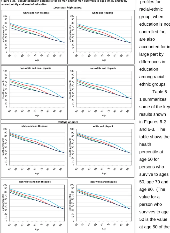
emphasize that much of the difference in health across racial-ethnic groups is
accounted for by differences in education, especially for men. In section 7 we simulate differences in survival probabilities by health and the level of education and use these estimates to show how the present discounted value (EDPV) of the payout from a fair annuity varies by gender, health, and level of education. Section 8 is a summary of our findings.
Section 2 Data and Descriptive Statistics
We first discuss the data used in the analysis and then describe the health index that is a key component of the analysis. We then show data on the variation in health at retirement ages by education and racial-ethnic groups and then discuss in some detail the evolution of health by level of education. Finally, we use the evolution of health for single and married persons to provide an alternative description of mortality selection and to highlight its quantitative importance.
The analysis uses data from the Health and Retirement Study (HRS). The HRS is a longitudinal survey that resurveys respondents every two years. The current HRS is comprised of five entry cohorts. The original HRS cohort surveyed respondents age 51 to 61 in 1992 and the Asset and Health Dynamics of the Older Old (AHEAD) cohort surveyed respondents age 70 and older in beginning in 1993. Subsequent cohorts
include the War Babies (WB) cohort first surveyed at ages 51 to 56 in 1998, the Children of Depression (CODA) cohort first surveyed at age 68 to 74 in 1998, and the Early Baby Boomers (EBB) first surveyed at ages 51 to 56 in 2004. Respondents are resurveyed every two years.
The HRS sampling methods can yield some non-representative demographic subsamples in the early years of the HRS. For example, the HRS cohort includes households with at least one person (the “age-eligible” person) born between 1931 and 1941 and their spouses. These age-eligible persons were age 51 to 61 when first surveyed in 1992. If an age-eligible person has a spouse, the spouse is automatically selected even if he or she is not age-eligible. In married households the women is, on average, younger than the man. As a result, there are more women at younger ages, for example ages 51 to 55, in the first few waves of the HRS than in the population.
This is because women who were under the age of 51 in 1992 but were married to age- eligible spouses will “age” into the sample in subsequent years. Thus in the second wave of the HRS there are few men less than age 53, but a substantial number of women. Moreover, none of these women are single (unless they were divorced, widowed, or separated since the previous wave) so the sample of women is highly unrepresentative of the general population. This aspect of the data is important to understanding some features of the model fit discussed in section 4.
The health index: One advantage of the HRS is the detailed information it provides on health conditions. We construct a health index based on the responses to 27 health-related questions concerning self-reported functional limitations, health
conditions, and medical care usage. The index is the first principal component of these 27 indicators. The full set of questions was not asked of all respondents in the HRS cohort in 1992 and the AHEAD cohort in 1993, however. Thus we have dropped all data for the first wave of the HRS and AHEAD cohorts. A more detailed description of the index and a list of included variables are contained in Poterba, Venti and Wise (2013). We note several important features of the index used in this paper. First, the index used in Poterba, Venti and Wise (2013) only included data through 2008. The index used in the present paper includes data through 2010. Second, the index used here is based on a pooled sample that includes all respondents from all HRS cohorts in
all years. The decision to pool was based on earlier experimentation with the index that showed little difference between estimates for men and women and little difference across years. The principal component loadings on the health variables were used to predict a raw health score for each respondent. This score was converted to a
percentile index with values from 1 to 100. A person’s percentile index value shows the person’s position relative to the health of all persons in all HRS cohorts in all years.
The index has several important properties for our analysis. First, it is strongly related to mortality. Figure 2-1 illustrates this for men and women using data from the earliest of the five HRS cohorts. These persons were age 51 to 61 in 1992 when first surveyed and age 53 to 63 in 1994. The figures show the percent of persons in each health decile in 1994 that were deceased by the year 2000 and the percent that were deceased by the year 2010. The figures show that the index strongly predicts mortality.
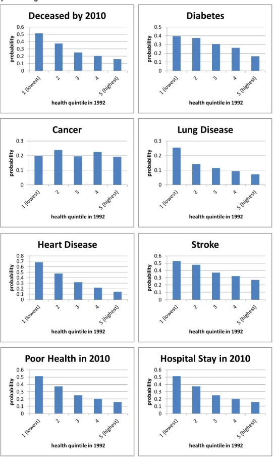
For example, over 71.6 percent of men (58.1 percent of women) in the poorest health decile in 1994 were deceased by 2010 but only 19.7 percent of men (10.3 percent of women) in the top health decile were deceased by 2010. Second, the index is strongly predictive of future morbidity as well. Figure 2-2 shows the percent of persons (of both genders) who report future health events such a stroke, the onset of diabetes, lung disease, and other health conditions. Persons in the poorest health decile in 1994 report higher incidence of each condition (with the exception of cancer) by 2010.
Figure 2‐1. Percentage deceased in 2000 and 2010 by health decile in 1994, persons age 53 to 63 in 1994
0 0.1 0.2 0.3 0.4 0.5 0.6 0.7 0.8
1 2 3 4 5 6 7 8 9 10
percent
health decile in 1992
Men
2000 2010
0 0.1 0.2 0.3 0.4 0.5 0.6 0.7 0.8
1 2 3 4 5 6 7 8 9 10
percent
health decile in 1992
Women
2000 2010
Figure 2-2. Probability of health events by 2010 by health quintile in 1994, all persons age 53 to 63 in 1994
0 0.1 0.2 0.3 0.4 0.5 0.6
probability
health quintile in 1992
Deceased by 2010
0 0.1 0.2 0.3 0.4 0.5
probability
health quintile in 1992
Diabetes
0 0.1 0.2 0.3
probability
health quintile in 1992
Cancer
0 0.1 0.2 0.3
probability
health quintile in 1992
Lung Disease
0 0.10.2 0.3 0.4 0.5 0.6 0.70.8
probability
health quintile in 1992
Heart Disease
0 0.1 0.2 0.3 0.4 0.5 0.6
probability
health quintile in 1992
Stroke
0 0.1 0.2 0.3 0.4 0.5 0.6
probability
health quintile in 1992
Poor Health in 2010
0 0.1 0.2 0.3 0.4 0.5 0.6
probability
health quintile in 1992
Hospital Stay in 2010
Variation in health after retirement: The index can also be used to show the variation in the health of persons near the age of retirement. Figure 2-3 shows how health varies by level of education for members of the original HRS cohort between 1994 and 2010. This figure is similar to Figure 2-1 in Poterba, Venti and Wise (2013) where details about how the figure was constructed are presented. The figure shows that large differences in health by level of education persist over time even as health declines for persons in all education groups. The slope of each line segment shows the health trajectory for persons alive at the beginning and end of each two-year interval.
The “gaps” between line segments are an indicator of mortality selection. These gaps are discussed below. When first observed at ages 53 to 63 in 1994, the differences in health by education group are very large. The mean health percentile in 1994 is 72.0 for persons with a college degree and 47.6 for persons with less than a high school degree. The key feature of the figures is that the level of health in subsequent years is largely determined by the level of health when first observed in 1994. Over time, health declines by approximately the same amount (in percentiles) for persons at all levels of education. This suggests that there is little effect of education on the change in health
0 10 20 30 40 50 60 70 80
health percentile
Year
Figure 2‐3. Mean health trajectories by level of education for persons age 53 to 63 in 1994
less then HS HS some college college or more
after 1994, the first year members of this cohort were observed. Poterba, Venti and Wise (2013) show similar figures for the AHEAD and the CODA cohorts of the HRS and for all persons age 65+ in 1998. Although there are some differences across the
groups, the basic pattern is the same for the cohorts.
Mortality selection: The observed age-health profile is the mean health in each year (or at each age) for all persons who survive to each year (age). Because of mortality selection, however, observed age-health profiles are an inaccurate
representation of how the health of persons evolves over time. Here we show how the age-health profile is distorted by selection. In the next section we describe a model to formally estimate and correct for mortality selection.
As noted above, there are two distinct processes that determine observed age- health profiles. The first is that persons become less healthy as they age. The
second—the selection effect—is that the least healthy are more likely to die and leave the sample. To isolate the role of selection we begin with a simple example where the first process is inoperative. Education (unlike health) does not change over time for persons in the HRS cohort. For any individual the age profile of education is flat (horizontal). However, the empirical age-education profile rises because of mortality selection—persons with lower education are more likely to die. Thus, for example, if we track married persons in the HRS cohort (age 53 to 63 in 1994) from 1994 to 2010 we find that mean years of education is 12.55 in 1994 and 12.89 in 2010. The difference of 0.34 years is purely the result of (cumulative) mortality selection.
We can also measure the extent of selection bias associated with each wave-to- wave transition in the HRS. Figure 2-4 shows average years of education of persons alive in consecutive waves in the HRS cohort between 1994 and 2010. Separate profiles are shown for single and for married persons. Each line segment in the figure shows the change in the education of persons alive in both the beginning year and the end year of the interval. Each of these segments is flat because the level of education of each person does not change over time. In this figure the observed age-education profile is the solid line connecting the end-points of each of the line segments for married persons. For example, the slope of the observed education profile between 1998 and 2000 is the difference between the mean education of all persons alive in
1998 (the last point of the 1996 to 1998 segment) and the mean education of all persons alive in 2000 (the last point of the 1998 to 2000 segment).
Some persons alive in 1998 did not survive to 2000. These persons are included in the 1996 to 1998 segment, but not in the 1998 to 2000 segment. Thus the education in 1998 of those who survived until 2000 is greater than the education of all persons who were alive in 1998, including those who did not survive until 2000. The difference is the mortality selection effect and it is identified in the figure as the vertical height of the gap between the end of the 1996 to 1998 segment and the beginning of the 1998 to 2000 segment. These gaps, of course, account for the upward slope of the observed age-education profile since the true age-education profile for individuals is flat. The sum of these gaps is the 0.34 years of education—the same selection effect reported above.
Health, unlike education, changes over time. Figure 2-5 shows a figure using health rather than education as the outcome variable. The height of the gaps is still a measure of the extent of mortality selection. However, if health is the outcome variable the segments are not flat—this reflects the decline of true health over time. For the period 1994 to 2010 the observed change in health—reflecting mortality selection and
the true change in health—is -15.6 percentile points (from the end year point of the 1994 to 1996 segment to the end year point of the 2008 to 2010 segment) for married persons. This can be decomposed into a “true” decline in health of -23.1 percentile points (the sum of the changes in slope segments) and a mortality effect of +7.5 percentile points (the sum of the gaps). The decomposition for single persons is quite similar. Over the 16 year period the observed decline in health is -18.0 percentile points. This is comprised of a “true” decline of -24.5 percentile points for survivors and a selection effect of 6.4 percentile points. These results pertain to persons in the original HRS cohort who were age 53 to 63 in 1994 and age 69 to 79 when last
observed in 2010. Similar calculations made for persons surviving to other ages show that selection effects are larger for persons at older ages. The average wave-to-wave selection effect is 0.93 for married persons, but this ranges from about 0.7 percentile points for the 1994 to 1996 interval to about 3.0 percentile points over the last two-year interval ending in 2010. Thus mortality selection is substantial at all ages and can lead to very misleading inferences about how health evolves in old age.
Section 3 The Model
Health: We begin with a description of the evolution of health from wave to wave.
In our framework is the true (unobserved) health for personiin periodt. We assume that true health is a function of observed individual characteristicsXitand an individual random term that captures the unobserved components of health and their evolution over time:
(3-1)
h
it X
it
H R
it
HThe random component allows for heterogeneity in health across persons as well as for persistence in health over time for the same person. It is specified to follow an AR(1) process with
(3-2) Rit Rit1uit
where is normalized to have mean zero and unit variance. The parameter captures the persistence of the unobserved component of health over time. In the special case that =1 the error structure is equivalent to a random effects model and the unobserved health component is constant over time. Noting that RitRit1uitand assuming that the process is stationary, then uit ~N(0, (12)). We then interpret the error term uit as capturing health shocks. Heiss (2011) weighs the relative merits of alternative error structures that can be used to accommodate persistence. We assume that the observed health indexHitis equal to true health measured with error:
(3-3)
H
it h
it e
it X
it
H R
it
H e
itWe treat the random termeitas measurement error with zero mean and variancee2—
~ (0, 2)
it e
e N . The total variance ofH, given observed covariatesX , is given by
2 2 2
( it | it) ( it) H ( )it H e V H X Var R
Var e
.Mortality: Mortality between periodt1and periodt is a function of individual characteristics in the prior periodXit1 and true health in the prior periodhit1. (Neither
X norh are defined for deceased persons in the present period). We assume that mortality (the likelihood of death) can be described by latent continuous variablemit, with
(3-4) mit Xit1
M hit1
M
itwhere is an error term with zero mean and unit variance and is uncorrelated with eit and uit, the error terms in the health equation. Substituting health hit1from equation (3-1), into 3-3 yields:
(3-4)
1
111 1
1
1
it H it H
H it H
i
it it M M it
it M M M it
i
it M t
M t
X
m X R
R
X R
X
whereM M HM and M HM.
Note that the total (reduced form) effect ofXit1 on mortality is given byM which can be decomposed into a “direct” effect Mand an “indirect” effect through health( HM). In summary: the health equation yields estimates ofHand H. The mortality equation yields estimates ofM and M. Given estimates ofH,M,H, and M we can recover
M M / H
andM M H( M /H).
Mortality selection occurs through both and . LetMit be a mortality indicator that that takes on the value one if a person dies between periods t1 andt, and zero otherwise. Following the conventional probit specification, we assume that Mit tales a value of one if latent mortality mit crosses a threshold (normalized to be zero), so Mit 1 if mit 0 or > -( + ). The probability that personi dies between t1 andt is then given by:
(3-6) Pr[Mit 1|Xit1,Rit1]
Xit1M Rit1M
where
is the standard normal cumulative distribution function.Conditional on the sequence
Ri1,...,RiT
, health and mortality are assumed to be independent over time, so if latent health were observed, the likelihood contribution of individual i would simply be(3-7) Pi
i1,..., iT
f( it| it, it) Pr[ it | it 1, it 1]t
R R
H X R M X R ,where f(Hit |Xit1,Rit) denotes the conditional density of observed health. The fact that respondents in the HRS are obviously alive when they enter the sample, has to be taken into account when integrating out the latent health process since mortality has created a more or less selected sample with respect to Rit, depending on the age and other covariates. We follow Heiss (2011) and explicitly derive the distribution of Rit conditional on survival to the first wave (Si1) when we do our likelihood calculations.
The likelihood contribution then becomes
(3-8) Li
Pi
Ri1,...,RiT
f R
i1,...,RiT Si1
dRi1dRiTThis integral could simply be approximated using Monte-Carlo simulation methods or multivariate numeric integration (Heiss and Winschel 2008). We use the sequential deterministic integration algorithm of Heiss (2008) since it is more accurate and less computational costly for this model class.
Mortality selection occurs because the unobserved components of the health and mortality equations are correlated. If the correlation is zero then there is no selection bias. If the correlation is negative then persons with higher health (given ) will have lower mortality and will be less likely to leave the sample via death. The covariance between unobserved components of the health and mortality equations (3-3 and 3-5) is:
1 1 1
,
2it H it it M it R H M
R e R v
Cov
,The correlation between the unobserved components is:
2
2 2 2 2 2 2 2 2 2 2
H M H M
R
R H e R M v H e M v
Section 4. Results
Joint Estimation Results: Results from the joint estimation of equations 3-3 and 3-6 are shown in Table 4-1a for women and Table 4-1b for men. Both equations
include the same set of covariates: 1) an age spline with breakpoints at ages 60, 70, 80 and 90, 2) a set of race-ethnicity indicators (the omitted group is white-non-
Hispanic), 3) indicator variables for the level of education attained (the omitted category
is less than a high school degree), and a variable indicating whether the respondent’s longest tenure job was blue collar.
Each table shows the estimated coefficients on covariates in the health and the mortality equations. The estimates for the mortality equation are the total effects (M) described above. (The total effect is decomposed into direct and indirect effects in Tables 4-3a and 4-3b below.) The probit estimates have been converted to marginal effects to make them easier to interpret. For each variable we calculate
i
i
j i
ij ij
P X
X X X
and then average over all observations (by gender). The exception to this rule is that we calculate marginal effects of the age spline variables by averaging over observations in the relevant age interval. The probit estimate of M has also been converted to a marginal effect in Table 4-1.
Coeffi-
cient z Coeffi-
cient z Coeffi-
cient z Coeffi-
cient z
Age
50-59 -1.269 -34.2 0.001 3.5 -1.455 -28.2 0.007 1.9
60-69 -0.986 -31.5 0.002 13.2 -1.121 -30.1 0.029 12.2
70-79 -1.417 -38.3 0.005 18.0 -1.634 -36.0 0.007 16.9
80-89 -2.004 -39.0 0.014 24.2 -2.066 -30.4 0.017 19.4
90+ -1.784 -13.1 0.023 13.9 -2.243 -12.4 0.020 7.3
White Hispanic -0.533 -0.7 -0.022 -3.7 1.060 1.1 -0.019 -3.2
Non-white non-Hispanic -6.467 -12.3 0.024 6.7 -3.237 -5.1 0.018 4.8 Non-white Hispanic -5.674 -4.6 -0.009 -0.9 -0.323 -0.2 -0.015 -1.5 Education
HS 9.006 16.9 -0.039 -11.5 5.321 8.5 -0.023 -6.4
Some college 11.958 19.3 -0.050 -12.1 7.378 10.2 -0.031 -7.4 college or more 18.206 25.0 -0.073 -14.7 16.545 20.4 -0.065 -14.1
Blue collar -2.503 -5.2 -0.004 -1.2 -1.785 -3.4 -0.015 -4.8
Intercept 55.769 91.6 65.356 80.1
e 9.403 205.6 9.442 154.9
H 25.526 137.4 25.863 117.5
M -0.086 -49.2 0.000 -41.6
0.941 766.2 N 88,326 0.931 543.9 N 64,812
Men Health effects
(βH)
Mortality effects (βM) Table 4-1. Joint estimates of health and mortality (marginal effects) for women and for men
Women Variable
Health effects (βH)
Mortality effects (βM)
The estimated marginal effect of the unobserved individual random term in the health and mortality equations, H andM respectively, are shown at the bottom of the tables. The effect of the unobserved health component is positive and statistically significant in the health equation (H) and is negative and statistically significant in the mortality equation (M).1 The estimated autocorrelation parameter () is greater than 0.93 for both men and women and suggests strong persistence in the unobserved component of health over time. The standard deviation of the measurement error in the health equation (e) is about 9.4 percentile points for both men and women. The correlations between the unobserved components of the health and mortality equation are -0.48 for women and -0.41 for men, verifying the strong mortality selection effect.
Health equation estimates: The effect of age on health is roughly similar for men and women. The estimates imply that health declines between one and 2 percentile points with each year of age. Health declines more rapidly at older ages than at younger ages and the estimated decline is more pronounced for men than for women.
The one unexpected pattern is that the estimate for ages 60-69 is slightly lower than the estimate for ages 50-59 for both men and women. The race-ethnicity estimates for women suggest that African-American health is 5.7 percentile points lower than the health of whites (among non-Hispanics). The Hispanic effect is quite small, about ½ of a percentile point less among whites and about one percent less among non-whites.
The race-ethnicity effects for men are smaller and less consistent. The non-white effect is -3.2 percentile points for non-Hispanics, but is negligible for Hispanics. The
1 To understand the estimate ofH, recall that V H( it|Xit)Var R( it)H2 Var e( )it H2 e2. The measurement error has mean zero and the estimated standard deviation is 9.40 for women and 9.44 for men. The estimate of H is 25.53 for women and 25.86 for men. The standard error of e is
approximately 9.4, so a one standard deviation change ineitwill change H by 9.4. The unobserved random term R is distributed N(0,1). Thus a one standard deviation change in R (a one unit change) will changeHbyRitHand is approximately 25. Then V H( it |Xit)H2 e2=625 + 88.36 = 713.36. Thus 87.6% of the unobserved variation in health given the covariatesX is explained by unobserved healthR
and 12.4% by measurement errore.
education-health gradient is large and statistically significant for both men and women.
For women, the health percentile of persons with a college degree or more is 18.2 points higher than the health percentile of persons with less than a high school degree (the omitted category). The difference for men is 16.5 percentile points. Primary employment on blue collar jobs is associated with lower health for both men and women. Although statistically significant, the estimates are much smaller than the estimated effects of education. Controlling for other covariates, the estimates for a blue collar job are -2.5 and -1.8 percentage points for women and men respectively.
Mortality equation estimates: The columns on the right side of Tables 4-1a and 4- 1b show the marginal effect of eachX variable on the probability that a respondent dies between the waves. These are the total (reduced form) effects from Equation 3-4. For women, mortality increases sharply with age—by one-tenth of one percent for each year of age between 50 and 59 and by about 2.3 percent for each year of age above 90.
The probability of death for men is greater than for women between ages 50 and 59 but lower than the probability for women at older ages. The one anomaly for which we have no explanation is the high (2.9 percent) estimate for men in the 60 to 69 age interval.
For both men and women, non-whites have higher mortality than whites and Hispanics have lower mortality than whites. That Hispanics have lower income and education than whites but live longer is known as the “Hispanic paradox” in the demographic literature (Scommegna 2013).
While primary employment on blue collar jobs is associated with lower health for both men and women, the relationship to mortality is different for men and women.
Controlling for education and other covariates, blue collar employment has little effect on mortality for women. However, a blue collar job is associated with a 1.5 percent decline in the probability of dying for men. As with health, however, the effect of
education on mortality is much greater than the effect of a blue collar job on mortality for both men and women. The difference in mortality of persons with less than a high school degree and those with a college degree or more is -7.3 percent for women and - 6.5 percent for men; the effect of a blue collar job is -0.4 percent for women (and not statistically significant) and -1.5 percent for men.
Joint Versus Single Equation Estimates of the Health Equation: The joint
estimates of health and mortality shown above “correct’ the parameter estimates in the health equation for mortality selection. Table 4-2 below reproduces these estimates and also shows single-equation estimates of the health equation. The key comparison is the estimated effect of age on health. For both men and women the estimated decline in health with age is greater in the two-equation model than in the single-
equation counterpart. This is consistent with mortality selection leading to an empirical health-age profile of survivors that declines less rapidly than the true decline in health with age. The joint estimates are slightly lower than the single equation estimates for most of the other covariates.
The Direct and Indirect Effect of Covariates and Unobserved Health on Mortality:
The estimated coefficients in the mortality equation (MandM) capture the “total”
(reduced form) effect of the covariatesX and unobserved healthRon mortality. Recall that we can decompose the total effect of each of the X covariates into its direct effect on mortality ( ) and the indirect effect through health ( ). We can also estimate the direct and indirect effects of R on mortality (Mand HM). The first column of Table 4-3a (for women) and Table 4-3b (for men) reproduces the total effects (probit estimates converted to marginal effects) of each X variable on mortality from Table 4-1.
variable coef-
ficient z coef-
ficient z coef-
ficient z coef- ficient z Age
50-59 -1.269 -34.2 -0.982 -20.3 -1.455 -28.2 -1.002 -15.8 60-69 -0.986 -31.5 -0.657 -19.1 -1.121 -30.1 -0.757 -19.4 70-79 -1.417 -38.3 -0.791 -20.1 -1.634 -36.0 -0.961 -21.2 80-89 -2.004 -39.0 -1.262 -22.8 -2.066 -30.4 -0.925 -12.5
90+ -1.784 -13.1 -0.476 -3.6 -2.243 -12.4 -0.666 -2.9
White Hispanic -0.533 -0.7 -1.470 -3.9 1.060 1.1 0.726 1.7
Non-white non-Hispanic -6.467 -12.3 -5.689 -23.7 -3.237 -5.1 -1.737 -5.8 Non-white Hispanic -5.674 -4.6 -5.848 -9.8 -0.323 -0.2 -0.107 -0.2 Education
HS 9.006 16.9 7.778 32.9 5.321 8.5 4.826 17.1
Some college 11.958 19.3 10.730 38.9 7.378 10.2 6.573 20.1 college or more 18.206 25.0 16.453 53.3 16.545 20.4 14.546 43.1 Blue collar -2.503 -5.2 -2.398 -10.8 -1.785 -3.4 -2.213 -9.4
Intercept 55.769 91.6 54.162 124.9 65.356 80.1 63.129 107.8
e 9.403 205.6 9.442 154.9
H 25.526 137.4 25.863 117.5
M -0.573 -49.2 -0.486 -41.6
0.941 766.2 0.931 543.9
R2 0.171 0.148
N 88,326 88,326 64,812 64,812
Table 4-2. Comparison of joint and single-equation estimates of parameters of the health equation
women men
joint estimates single equation
estimates joint estimates single equation estimates
The next two columns show the calculated direct effects and the indirect effects (through health) for each of the X variables.
coeff- z coeffi- z coeffi- z
Age
50-59 0.001 3.5 -0.004 -0.1 0.004 28.4
60-69 0.002 13.2 -0.001 7.5 0.003 26.7
70-79 0.005 18.0 0.000 8.4 0.005 30.5
80-89 0.014 24.2 0.008 11.1 0.007 31.0
90+ 0.023 13.9 0.017 7.0 0.006 12.7
White Hispanic -0.022 -3.7 -0.024 -4.6 0.002 0.7
Non-white non-Hispanic 0.024 6.7 0.002 0.8 0.022 11.9
Non-white Hispanic -0.009 -0.9 -0.028 -3.2 0.019 4.6
Education
HS -0.039 -11.5 -0.009 -3.2 -0.030 -15.9
Some college -0.050 -12.1 -0.010 -2.8 -0.040 -18.0
college or more -0.073 -14.7 -0.012 -2.9 -0.061 -22.3
Blue collar -0.004 -1.2 -0.013 -4.1 0.008 5.2
Variable Total Effect ( ) Direct Effect ( ) Indirect Effect ( ) Table 4-3a. Estimated effects of X variables on mortality for women - total, direct, and indirect (through health) effects
γ̃
coeff- z coeffi- z coeffi- z
Age
50-59 0.007 1.9 0.003 -1.5 0.004 23.5
60-69 0.029 12.2 0.026 6.5 0.003 24.6
70-79 0.007 16.9 0.002 7.8 0.004 27.4
80-89 0.017 19.4 0.011 10.0 0.006 24.7
90+ 0.020 7.3 0.014 2.3 0.006 12.0
White Hispanic -0.019 -3.2 -0.016 -3.1 -0.003 -1.1
Non-white non-Hispanic 0.018 4.8 0.009 2.9 0.009 5.0
Non-white Hispanic -0.015 -1.5 -0.016 -1.8 0.001 0.2
Education
HS -0.023 -6.4 -0.008 -2.8 -0.015 -8.3
Some college -0.031 -7.4 -0.011 -3.1 -0.020 -9.8
college or more -0.065 -14.1 -0.020 -5.1 -0.045 -18.1
Blue collar -0.015 -4.8 -0.020 -7.6 0.005 3.4
Table 4-3b. Estimated effects of X variables on mortality for men - total, direct, and indirect (through health) effects
Variable Total Effect ( ) Direct Effect ( ) Indirect Effect ( )γ̃
For the most part each covariate has both direct and indirect effects on mortality.
Perhaps the most striking result of the decomposition is for education. The total effect of education on mortality is quite substantial for both men and women, but the direct effect is small; most of the effect of education on mortality is indirect (through the effect of education on health). For women, between 77.3 and 84.4 percent of the total effect of education on mortality is through health; for men between 64.3 and 69.7 percent is through health. It is also striking that the lower mortality of Hispanics (the Hispanic paradox) is almost exclusively a direct effect. The indirect effect through health is small and not statistically significant for either men or women. As noted above, a surprising result is that controlling for education and other covariates, blue collar employment has little effect on mortality for women but is associated with a 1.5 percent decline in the probability of dying for men.
Section 5 Simulations: Model Fit, Mortality Selection and Health Dynamics We use simulations to verify the model fit, to describe the measurement of mortality selection, and to demonstrate the dynamic properties of health.
The Model Fit: We perform several simulations to assess the fit of the model.
Each simulation is based on 1,000 replications for each person in the original HRS data set. Health-age profiles for each replicated person are simulated from age 50 until death. The race/ethnicity, education and occupation variables remain constant over time. To simulate the unobserved components at age 50 we draw uitfrom its estimated distribution with mean zero and variance(12) and draw
it from its estimateddistribution with mean zero and unit variance. As we simulate forward we make new draws of uit and
it from their respective distributions to generate the latent processRit. The simulation yields a value for Hit and a probability of death,Pr[Mit 1|X Rit, it], in each period. At each age persons are randomly dropped from the sample with
probabilityPr[Mit 1|X Rit, it].
10 20 30 40 50 60 70 80
50 52 54 56 58 60 62 64 66 68 70 72 74 76 78 80 82 84 86 88 90 92 94 96 98
Health percentile
Age
Figure 5‐1a. Actual and simulated health percentile for all women and for women surviving to ages 70, 80, and 90
survive to 70 (actual) survive to 80 (actual) survive to 90 (actual) all (actual) survive to 70 (sim) survive to 80 (sim) survive to 90 (sim) all (sim)
10 20 30 40 50 60 70 80
50 52 54 56 58 60 62 64 66 68 70 72 74 76 78 80 82 84 86 88 90 92 94 96 98
Health percentile
Age
Figure 5‐1b. Actual and simulated health percentile for all men and for men surviving to ages 70, 80, and 90
survive to 70 (actual) survive to 80 (actual) survive to 90 (actual) all (actual) survive to 70 (sim) survive to 80 (sim) survive to 90 (sim) all (sim)
0 0.05 0.1 0.15 0.2 0.25 0.3 0.35 0.4
50 52 54 56 58 60 62 64 66 68 70 72 74 76 78 80 82 84 86 88 90 92 94 96 98
Health percentile
Age
Figure 5‐2a. Actual and simulated mortality rate for women
simulated actual
0 0.05 0.1 0.15 0.2 0.25 0.3 0.35 0.4
50 52 54 56 58 60 62 64 66 68 70 72 74 76 78 80 82 84 86 88 90 92 94 96 98
Health percentile
Age
Figure 5‐2b. Actual and simulated mortality rate for men
simulated actual
To show the model fit we have “reproduced” by simulation Figure 1-1 that shows the average health percentile at each age based on HRS data. Figures 5-1a and 5-1b below compare the observed health profile with the simulated profile for men and women respectively. The figures compare both the average age-health profile (labeled
“all”) as well as the prior health profiles of persons who survived to age 70, to age 80, and to age 90. The actual and the simulated profiles correspond very closely.
Figures 5-2a and 5-2b compare actual and simulated mortality rates by age for women and men respectively. The actual mortality rates come from the Social Security period life table for 2007. Again, the two profiles correspond quite closely.
Measuring Mortality Selection: We emphasized above the two distinct processes that determine observed age-health profiles—the first is that persons become less healthy as they age and the second, the selection effect, is that the least healthy are more likely to die and leave the sample. Simulations based on our model can help to understand the magnitude of the selection effect as well as other implications of mortality selection. The observed age-health profile of survivors is the sum of the effects of these two processes and is given by
H
it X
it
H R
it
H e
it, where the measurement errore
it has mean zero at all ages. This profile is shown by the heavy solid line in Figure 5-3a (women) and Figure 5-3b (men). This is the simulated value ofHitfor persons who have survived to each age and is the same profile shown earlier as the fitted lines in Figures 5-1a and 5-1b. The blue dashed profile in these figures is the average value of the unobserved component
R
it
H of the health of survivors andmeasures the extent of mortality selection. The first process—the decline in health with age—is shown by the dashed red line which isHitminus the unobserved component
R
it. This is the mortality corrected age-health profile. By age 80 the observed age-health profile understates the decline in health by about 8.8 percentile points for women and 10.7 percentile points for men.
0 10 20 30 40 50 60 70 80
50 52 54 56 58 60 62 64 66 68 70 72 74 76 78 80 82 84 86 88 90
Health percentile
age
Figure 5‐3a. Simulated components of the observed health‐age profile for women
mean unobserved component (R) corrected for mortality selection simulated health‐age profile
0 10 20 30 40 50 60 70 80
50 52 54 56 58 60 62 64 66 68 70 72 74 76 78 80 82 84 86 88 90
Health percentile
age
Figure 5‐3b. Simulated components of the observed health‐age profile for men
mean unobserved component (R) corrected for mortality selection simulated health‐age profile