The Benefits of India’s Rural Roads Program in the Spheres of Goods, Education and Health

Policy Research Working Paper 6169

The Benefits of India’s Rural Roads Program in the Spheres of Goods, Education

and Health

Joint Estimation and Decomposition

Clive Bell

The World Bank South Asia Region Transport Unit

WPS6169

Public Disclosure AuthorizedPublic Disclosure AuthorizedPublic Disclosure AuthorizedPublic Disclosure Authorized

Abstract

The Policy Research Working Paper Series disseminates the findings of work in progress to encourage the exchange of ideas about development issues. An objective of the series is to get the findings out quickly, even if the presentations are less than fully polished. The papers carry the names of the authors and should be cited accordingly. The findings, interpretations, and conclusions expressed in this paper are entirely those of the authors. They do not necessarily represent the views of the International Bank for Reconstruction and Development/World Bank and its affiliated organizations, or those of the Executive Directors of the World Bank or the governments they represent.

Policy Research Working Paper 6169

All-weather rural roads usually improve not only villagers’

terms of trade, but also their educational attainments and health. Obtaining empirical estimates of the benefits generated by the first is straightforward, not so those generated by the others. The object of this paper is to estimate the relative sizes of their respective contributions to total benefits in connection with the all-India rural roads program Pradhan Mantri Gram Sadak Yojana, using an overlapping generations model featuring the production and consumption of goods and the formation

This paper is a product of the Trasnport Unit, South Asia Region. It is part of a larger effort by the World Bank to provide open access to its research and make a contribution to development policy discussions around the world. Policy Research Working Papers are also posted on the Web at http://econ.worldbank.org. The author may be contacted at clive.bell@urz.

uni-heidelberg.de.

of human capital in the presence of both morbidity and mortality. Based on survey evidence from upland Orissa in India and Bangladesh, as well as elements of more usual forms of calibration, the model yields a ratio of commercial to non-commercial benefits of about two-to-one in the first generation, falling to three-to- four in the second. This is broadly consistent with the valuations expressed by respondents in the Orissa survey, who ranked the latter benefits at least on a par with the former.

The Benefits of India’s Rural Roads Program in the Spheres of Goods, Education and Health: Joint

Estimation and Decomposition

Clive Bell

(Appendix by Jochen Laps)

First version: January, 2010. This version: August, 2012

Abstract

All-weather rural roads usually improve not only villagers’ terms of trade, but also their educational attainments and health. Obtaining empirical estimates of the benefits generated by the first is straightforward, not so those generated by the others. The object of this paper is to estimate the relative sizes of their respective contributions to total benefits in connection with the all-India ru- ral roads program Pradhan Mantri Gram Sadak Yojana, using an overlapping generations model featuring the production and consumption of goods and the formation of human capital in the presence of both morbidity and mortality.

Based on survey evidence from upland Orissa in India and Bangladesh, as well as elements of more usual forms of calibration, the model yields a ratio of com- mercial to non-commercial benefits of about two-to-one in the first generation, falling to three-to-four in the second. This is broadly consistent with the val- uations expressed by respondents in the Orissa survey, who ranked the latter benefits at least on a par with the former.

Keywords: Rural roads, transport costs, education, health, India JEL Classification: E62, O19, O12

Sector Board: Transport

∗University of Heidelberg, INF 330, D-69120 Germany. This paper was prepared as part of the documentation for a World Bank loan proposal in connection with PMGSY. The views expressed herein are not, however, necessarily those of the World Bank or its Board.

1 Introduction

A new all-weather rural road will bring various benefits to the villagers along its route.

As producers, they will enjoy higher net prices for their marketed surpluses; as con- sumers, they will pay less for urban goods. If there is no school in the village itself, those children who already attend one elsewhere will spend less time traveling to and fro, and those who did not attend earlier may do so now. If there is a village school, it is the teachers themselves who may appear more regularly. Much the same holds for medical treatment. Children and those adults with chronic ailments are more likely to make regular visits to the clinic; and in an emergency, those in need of medical atten- tion will be able to reach the clinic sooner, which may make the difference between life and death.

Measuring the road’s effects on these movements of goods and people is, in principle at least, relatively straightforward. Valuing the resulting benefits is another matter altogether. For the new road affects not just the decisions of what to produce and consume in the sphere of what might be called ‘textbook goods’, but also those having to do with the formation and maintenance of human capital, including life itself. These decisions are not, moreover, readily separable, which calls for their analysis within a unified framework. Yet more is at stake than consistency and rigor. It will be argued that valuing the benefits that arise in connection with more favorable prices of goods, improved educational attainment and lower morbidity involves a common (money) metric which is directly related to effects that are fairly readily measurable – provided families decide not to educate their children fully. In contrast, the benefits of reduced mortality, even if such reductions can be measured with some confidence, do not fit into this convenient scheme of things. The same will hold, moreover, if children are fully educated. How, then, are these benefits to be estimated in practice? A unified framework, in which decisions in the spheres of production, consumption and education are made in a particular environment of morbidity and mortality, provides one way of answering this question. For one can set up the model so that, counter-factually, the road lowers transport costs but nothing else; or, at the other extreme, everything else but transport costs. Granted that the model can be numerically calibrated, one can use the equivalent variation (EV) for each setting, relative to the benchmark of ‘no- road’, to establish the size of the benefit arising from lower transport costs relative to those arising from other effects. Since estimating the money-metric benefits of lower transport costs is a relatively straightforward task and does not involve the apparatus of a unified model, combining such an estimate with the corresponding contribution

to the total benefit, as yielded by the model, will then yield an estimate of the total benefit that has a substantial empirical anchoring.

The object of this paper is to estimate therelative size of the contribution of reduced transport costs, in connection with the all-India rural roads program known asPradhan Mantri Gram Sadak Yojana (PMGSY), a very large scheme that will eventually cover some 170,000 habitations, take at least 20 years to implement and cost in excess of US$40 billion (World Bank, 2010). The unified framework employed for this purpose is the overlapping generations (OLG) model of Bell, Bruhns and Gersbach (2006), sub- stantially extended so as to cover transport costs and morbidity. Important elements of the empirical basis for this application are supplied by an analysis of a survey of some 240 households drawn from 30 villages lying in the upland – and poor – region of Orissa (Bell and van Dillen, 2012) and two large surveys in Bangladesh (Khandker et al., 2009). There is also an indirect check, in the form of completely independent estimates of the so-called value of a statistical life provided by Lui et al. (1997) and Simon et al. (1999).

The plan of the paper is as follows. The model is set out and analyzed in Section 2, the essential difficulty with valuing the benefits arising from effects other than those of lower transport costs being addressed in Section 2.3. The numerical set-up follows in Section 3, which is divided up into subsections dealing with functional forms, parameter values and calibration under perfect foresight. This is the basis for the exact welfare analysis in Section 4, treating in sequence the benchmark of ‘no-road’, the world with the road and the contribution of lower transport costs to the whole resulting benefit.

The conclusions are drawn together in Section 5.

2 The Model

The basis is the model of Bell, Bruhns and Gersbach (2006), which deals with human capital formation and growth when there is premature adult mortality. To summarize, an extended family comprises three overlapping generations, with all surviving adults caring for all related children in each period, which stretches over a generation.¹ The young adults are assumed to decide how current resources are to be allocated between consumption and the children’s education. The level of current resources available to

1This arrangement is admittedly a rather idealized description of the social structure even in Kenya, let alone in rural India, but the pooling of the risks of premature mortality among the adults greatly simplifies the analysis.

the family is largely determined by the level of the parents’ human capital and their survival rate, but the children themselves can also work instead of attending school.

At the end of each period, some young adults die prematurely, all old adults die, and the children are on the point of becoming young adults.

How much of childhood, if any, is spent at school depends not only on the family’s available resources, but also on three further factors. First, there is the parents’ desire to provide for their old age and their children’s future, motives which express themselves in the parents’ willingness to forego some current consumption in favour of investment in their children’s schooling, and hence of the children’s human capital when they attain adulthood in the next period. Second, there is the efficiency with which schooling is transformed into human capital, which arguably depends on the quality of the school system and child-rearing within the family, whereby the latter ought to improve with the parents’ human capital. Third, the returns to the investment in any child will be effectively destroyed if that child dies prematurely in adulthood. This implies that the expected returns to education depend on parents’ (subjective) assessments of the probability that their children will meet an untimely death.

For present purposes, we need to extend this framework in two ways. First, the transportation of goods and persons must be brought into the picture. Instead of the aggregate consumption good in Bell, Bruhns and Gersbach (2006), there are now two consumption goods, one of which the household produces; the other is an ‘urban’ good, which the household can obtain only through exchange. The resulting trade necessar- ily involves transportation. The same holds for education and health, insofar as the children and their teachers must travel to school and the sick to a clinic, which may lie some distance off and, in the absence of an all-weather road, be inaccessible at times.

Second, we introduce morbidity, which, as formulated below, reduces individuals’ ca- pacities to go about their daily business.

2.1 Human capital and output

We begin by introducing some notation.

N_t^a: the number of individuals in the age-group a(= 1,2,3) in periodt, λ^a_t: the human capital possessed by an adult in age-group a(= 2,3), γ: the human capital of a school-age child,

α_t: the output produced by a unit of human capital input in year t,

e_t: the proportion of their school-age years actually spent in school by the cohort of children (a= 1) in period t.

Human capital is formed through a process that involves the adults’ human capital and the educational technology. The human capital attained by a child on becoming an adult in period t + 1 depends, in general, on the numbers and human capital of the adults, the level of schooling that child received, and the number of siblings of school-going age, who were presumably competing for the adults’ attention, care and support – all in the previous period. Formally,

λ²_t+1 = Φ(e_t,λt,N_t), (1) where λt = (λ²_t, λ³_t) and N_t = (N_t¹, N_t², N_t³) and Φ is increasing in all its arguments, except for N_t¹.

Simplifying with the application in mind, let Φ be multiplicatively separable in: (i) the educational technology, which involves only e_t; (ii) the average level of the adults’

human capital; and (iii) the degree of competition among siblings. This implies that formal education and the adults’ human capital are complements in producing the children’s human capital, which is intuitively plausible.² Parents in rural India have most of their children when they are in their twenties, and in their thirties, they are busy rearing them to adulthood. Normalizing the structure to a representative couple within the extended family, these assumptions yield the following specialization of (1):

λ²_t+1 =f_t(e_t)· 2(N_t²λ²_t +N_t³λ³_t) N_t²+N_t³ ·ψ

N_t¹

N_t²+N_t³

+ 1, (2)

wheref_t(·) represents the educational technology, whose efficiency may vary with time, and the function ψ(·) the effects of competition among siblings for their parents’ time and attention. These functions are assumed to have the following properties: f_t(·) is continuous and increasing ∀e_t ∈ [0,1), with f_t(0) = 0; and ψ(·) is continuous and de- creasing in the number of children per adult, and goes to zero as that number becomes arbitrarily large. The assumption f_t(0) = 0 implies that a child who receives no school- ing will attain only some basic level of human capital, which, without loss of generality, may be normalized to unity – hence the ‘1’ on the RHS of (2). The assumption that ψ(·) is a decreasing function implies that, cet. par., an increase in mortality among parents that outweighs any reduction in fertility will hinder the formation of human

2Becker, Murphy and Tamura (1990) and Ehrlich and Lui (1991) pioneered the approach based on the direct transmission of potential productivity from parent to child.

capital among their children. Let there be no depreciation of human capital.

The difference equation (2) governs the system’s dynamics. A brief remark will suffice on the asymptotic behaviour of λ²_t when there is full education. Observe that under stationary technological and demographic conditions, (2) may be written as

λ²_t+1 = 2f(e_t)(a₂λ²_t +a₃λ²_t−1) + 1,

where a₂ and a₃ are constants and λ²_t−1 =λ³_t. Suppose e_t = 1∀t, so that the relevant characteristic root isa₂[1+

(1+2a₃/(a²₂f(1)))]f(1). Then, starting from a sufficiently large value of the parents’ combined human capital, when they would choose e_t = 1, unbounded growth of λ²_t is possible if a₂[1 +

(1 + 2a₃/(a²₂f(1)))]f(1) ≥ 1, and the inter-generational growth rate then approaches

g^∗ ≡a₂[1 +

(1 + 2a₃/(a²₂f(1)))]f(1)−1, (3) from above. If, however, 1 > 2(a₂ +a₃)f(1), λ²_t will approach the stationary value 1/[1−2(a₂ +a₃)f(1)]. It should be remarked that if e_t is restricted below unity, to

¯

e_t say, then the latter value will replace unity as the argument of f(·) in the above expressions. This will be important when analysing the long-run effects of morbidity, travelling to school and involuntary absences in Sections 3 and 4.

The household produces a single consumption good (good 1) solely by means of labor, measured in efficiency units, under constant returns to scale. A natural normalization is that a healthy adult who possesses human capital in the amountλ^a_t is endowed withλ^a_t efficiency units of labor, which he or she is assumed to supply completely inelastically.

To accomodate sickness and injury, denote the fraction of each period that a surviving adult spends in disability by d^a_t(a= 2,3). Children, too, suffer ailments, which reduce the effective time left for schooling and work. Each child supplies (1−d¹_t−(1 +τ)e_t)γ efficiency units of labor when it spendse_tunits of time in school and, unavoidably, τ e_t units of time travelling to and from school, whereby γ ∈(0,1), i.e., a full-time working child is less productive than an uneducated adult. The household therefore produces

y_1t=α_t

N_t¹(1−d¹_t −(1 +τ))e_t)γ+ (1−d²_t)N_t²λ²_t + (1−d³_t)N_t³λ³_t

(4) units of good 1 in period t.

2.2 The family’s preferences and decisions

Some additional notation is needed.

x_it: the consumption of goodi(= 1,2) by each young adult,

β: the proportion of a young adult’s consumption received by each child, ρ: the proportion of a young adult’s consumption received by each old adult, σ_t: the direct costs per child of each unit of full-time schooling,

n_t: the number of children born to a representative couple who survive to school age in period t,

xq_a: the probability that an individual aged a will die before reaching the age of a+x,

q_t: the probability that a young adult in period t will die before reaching the third phase of life.³

The parameters β and ρare viewed as binding by all concerned through a social norm and they are enforced by appropriate social sanctions.

The extended family’s expenditure-income identity involves, in principle, outlays on the two consumption goods, health care and education, where the latter include both the direct expenditures and the opportunity costs of the pupils’ time. In what follows, we resort to the drastic simplification that there are no expenditures on getting to the clinic and being treated: mortality and morbidity rates are set exogenously, at levels that depend on the availability or otherwise of an all-weather road. This is not merely simplification in the interests of making the analysis more tractable. For the relationship between choosing treatment and the experience of disability over the whole stretch of a generation is not only difficult to model, but is also not well-established empirically: for example, better access to a clinic may induce timelier and heavier outlays on treating an acute ailment, and so save outlays on undoing even more damage later, should the condition go untreated at the outset.

It will be convenient to normalize the budget identity by the number of young adults.

The said identity may then be written as:

P_t(β, ρ)·p_t·x_t+Q_t(α_t, γ, σ_t, τ)·e_t≡p_1tα_t·(Λ_t+N_t¹(1−d¹_t)γ)/N_t², (5)

3In the present structure, this statistic corresponds to₂₀q20, the probability that an individual will die before 40, conditional on surviving until 20.

where the household faces the price vector p_t for the two consumption goods and Λ_t≡N_t²(1−d²_t)λ²_t +N_t³(1−d³_t)λ³_t (6) is the adults’ aggregate supply of efficiency units of labor. The term

P_t(β, ρ)≡(1 + (ρN_t³+βN_t¹)/N_t²) (7) expresses the effect of the family’s demographic structure on the ‘price’ of the con- sumption bundle x_t relative to education. Analogously, the ‘price’ of a unit of full education (e_t = 1) is

Q_t ≡(p_1tα_t(1 +τ)γ+σ_t)N_t¹/N_t². (8) The RHS of (5) is the level of (normalized) full income in period t. In this connection, observe that N_t¹, N_t² and N_t³ are related as follows:

N_t¹ =n_tN_t²/2, (9)

N_t² =n_t−1N_t−1² /2, (10)

N_t³ = (1−q_t−1)N_t−1² . (11) The young adults’ preferences are, in principle at least, defined over the following: the levels of consumption in young adulthood and old age, x_t and ρx_t+1, respectively, and the human capital attained by their school-age children on attaining full adulthood (λ²_t+1), which they may appreciate in both phases of their own lives. Investment in the children’s education therefore produces two kinds of pay-offs, one altruistic, as expressed by the value directly placed on λ²_t+1, and the other selfish, inasmuch as an increase in λ²_t+1 will also lead to an increase in ρx_t+1 under the said social rules.

Although the pooling arrangement implicit in the extended family structure elimi- nates the risk that orphaned children will be left to fend for themselves, others remain.

A young adult still faces uncertainty about whether he or she will actually survive into the last phase of life, and whether his or her children will do likewise, conditional on their reaching adulthood in their turn. The incidence of morbidity is uncertain at the level of the individual, though if the extended family is large enough, its realized levels of morbidity will differ little from the population rates. There is also uncertainty about future demographic developments, which will influence the realized level of ρx_t+1.

At the start of period t, young adults choose like partners. Each couple produces n_t

children, and then draws up a plan for current consumption and investment in the chil- dren’s education based on the family’s resources and expectations about its members’

state of health and other relevant variables in the coming and future periods. Given such assortative mating, the pair will agree wholly on what is to be done. Appealing to the law of large numbers in order to rid the system of any uncertainty about the real- ized levels of morbidity in period t, so that full income in that period is non-stochastic, let the preferences of a young adult at time t be represented as follows:

E_tU =b₁u(x_t) +b₂(1−q_t)E_t[u(ρx_t+1)] +E_t[(1−q_t+1)]·n_tφ(λ²_t+1), (12) where goods 1 and 2 are private goods in consumption, but the children’s attainment of human capital is a public one within the union. It should be noted, first, that no account has been taken of the pain and suffering associated with morbidity, even though its level may change exogenously; second, that the ‘pay-offs’ in the event that the parent should die prematurely (with probability q_t), or that any of the children, in their turn, should die prematurely in adulthood (each with probabilityq_t+1), have been normalized to zero; and third, that conditional on surviving into old age at t+ 1, the associated level of consumption, ρx_t+1, is also a random variable viewed at timet, for its level depends on a whole variety of future economic and demographic developments.

Finally, observe also that the parents’ altruistic motive makes itself felt only when they themselves are young and actually make the sacrifices, whereby λ²_t+1 is non-stochastic by virtue of e_t being non-stochastic.

These adults take all features of the environment in periods t and t+ 1 as paramet- rically given. It will be helpful to distinguish between what they know and what they must forecast. At the time of decision, the current endowment and environment are described by the vector

Z_t≡(N_t, n_t,λt, P_t, Q_t,p_t, τ, α_t, q_t,d_t). (13) This is assumed to be known.⁴ What is unknown are the (future) realizations of x_t+1 andq_t+1. Under the social norm expressed byρ, the parents attmust form expectations about how their surviving children will allocate full income in period t+ 1, a decision that depends, not only on Z_t+1, which will have been revealed at that time, but also on all future constellations thereafter, to the extent that these influence (x_t+1, e_t+1).

4It can be argued that there is uncertainty aboutq_t at the point of decision at timet, the (indi- visible) unit period being rather long. This possibility is addressed below.

For simplicity, all individuals’ forecasts of all elements of the future environment are assumed to be point estimates, so that whilst there is uncertainty about an individual’s personal fate, there is none about the future mortality profile itself or future fertility.

Indeed, we go farther down this path, and assume not only that all individuals share the same forecasts of {Z_t+1}^t=∞_t=1 , but also that these forecasts are unerring: that is to say, there is perfect foresight about everything – with the vital exception of whether a particular individual will die prematurely. Under this assumption, ρx_t+1 becomes non-stochastic, conditional on surviving into old age at timet+ 1, so that (12) may be written

E_tU =b₁u(x_t) +b₂(1−q_t)u(ρx⁰_t+1) + (1−q_t+1)·n_tφ(λ²_t+1(e_t)), (14) where the superscript ‘0’ denotes the optimal choice of those making decisions at time t+ 1, which their parents forecast unerringly at t. The functions u and φ are assumed to be strictly concave.

A young adult’s decision problem therefore takes the following form:

max

(xt, et|{Z_t+t}^t_t^=∞₌₀ )

E_tU s.t. x_t ≥0, e_t∈[0,(1−d¹_t)/(1 +τ)],(2),(5). (15) Iff_t¹(·) is concave, E_tU(·) will be strictly concave in (x_t, e_t). Hence, problem (15) has a unique solution and the first-order necessary conditions are also sufficient. Observe that the optimum always involves x_t>0. The corner solution in which the children are not educated at all can also be ruled out when f(·) satisfies the lower Inada condition, since ∂λ²_t+1/∂e_t is then unbounded at e_t= 0; but this condition will not be imposed.

2.3 Comparative statics

The associated Lagrangian is, omitting the non-negativity constraints for brevity, L=b₁u(x_t) +b₂(1−q_t)u(ρx⁰_t+1) + (1−q_t+1)·n_tφ(λ²_t+1(e_t))

+μ

p_1tα_t·(Λ_t+N_t¹(1−d¹_t)γ)/N_t²−P_t(β, ρ)·p_t·x_t−Q_t(α_t, γ, σ_t)·e_t

. (16)

The Envelope Theorem yields the following results, all of which accord with elementary intuition. Where the movement of goods and school children is concerned, we have

∂E_tU⁰

∂p_1t =μ

α_t·(Λ_t+N_t¹(1−d¹_t)γ)/N_t²−P_t(β, ρ)·x_1t−(α_t(1 +τ)γN_t¹/N_t²)e_t

>0, (17)

and ∂E_tU⁰

∂p_2t =−μP_t(β, ρ)·x_2t<0, (18) by virtue of the fact that the household is a net seller of good 1 and a net buyer of good 2, and e_t≤(1−d¹_t)/(1 +τ). An increase in the travel-time to school is likewise damaging. Denoting by ν the multiplier associated with e_t ≤(1−d¹_t)/(1 +τ)≡¯e_t,

∂E_tU⁰

∂τ =−μp_1tα_tγ(N_t¹/N_t²)e_t−ν(1−d¹_t)/(1 +τ)². (19) Morbidity reduces not only the family’s productive endowments, pain and suffering having been ruled out by assumption, but also ¯e_t:

∂E_tU⁰

∂d¹_t =−μp_1tα_tγ·(N_t¹/N_t²)−ν/(1 +τ), (20)

∂E_tU⁰

∂d²_t =−μp_1tα_t·λ²_t, (21)

∂E_tU⁰

∂d³_t =−μp_1tα_t·(N_t³/N_t²)λ³_t. (22) Turning at last to mortality, we begin by recalling (11); so that q_t exerts an influence on E_tU, not only directly, but also on the feasible set in period t + 1, and hence on x⁰_t+1. We have

∂E_tU⁰

∂q_t =−b₂u(ρx⁰_t+1) +b₂(1−q_t)∇u(ρx⁰_t+1)·

ρ∂x⁰_t+1

∂q_t

; (23)

and ∂E_tU⁰

∂q_t+1 =b₂(1−q_t)· ∇u(ρx⁰_t+1)·

ρ∂x⁰_t+1

∂q_t+1

−n_tφ(λ²_t+1(e_t)), (24) which reflects the fact that an increase in premature mortality among the children on reaching adulthood will also affect the parents’ consumption in old age, should they survive to enjoy it. In this connection, note that an increase in q_t+1 may well induce an increase in x⁰_t+1, since higher premature mortality in any period makes old-age provision for the next less attractive.

3 Setting up the System Numerically

The benefits flowing from an all-weather road stem from more favorable prices facing the household as producer and consumer, from reduced time for the children to go to and from school, and from lower morbidity and mortality due to timelier treatment.

Under the above assumptions, it is seen from (17) - (22) that, with the exception of re- duced mortality, sufficiently small changes in each of these features of the ‘environment’

yield benefits that, in money-metric utility, are equal to the gains or savings calculated at the allocation ruling before the said change and valued at the corresponding oppor- tunity cost.⁵ Inspection of (23) and (24), however, reveals that there is no such ready simplification where mortality is concerned; for the sub-utility functionsuandφappear explicitly, as does the next bundle, x⁰_t+1, in the perfect-foresight sequence {x⁰_t}^t=∞_t=0 . In order to obtain some feel for the size of the value placed on reduced mortality relative to that of other benefits, a resort to some numerical examples is unavoidable. This task involves the construction of the whole perfect-foresight sequence.

3.1 Functional forms

There is no hope of estimating more than a tiny part of this system econometrically;

and even ‘calibration’ for the system as a whole is ruled out for want of suitable data.

The approach, therefore, is to choose functional forms that are both tractable and plausible, if only through common usage in other contexts, and then constellations of associated parameter values such that certain key magnitudes correspond to what are called the ‘stylized facts’.⁶

1. Technologies. Let f_t(e_t) = z_te_t ∀t, where z_t represents an inter-generational trans- mission factor, which reflects the quality of both child-rearing and the school system.

This limiting form is certainly the simplest, and it causes no technical problems in view of the assumption that φ is strictly concave (see below). The absence of diminishing returns does not seem especially odd when one reflects on the need for children to spend some years in school before they have mastered the three R’s, which form the basis of all other acquired abilities involving literacy. The great majority of school-children in

5Observe that ifν = 0, each of these expressions is scaled by the Lagrange multiplierμ. As it turns out, this simplification is lost after period 1, whenν >0; so that the whole apparatus is also needed in connection with chnages in trip-time and morbidity.

6As Solow once wrote in the original connection with the character of growth in industrialized countries in the decades following WWII, they are certainly stylized, but whether they are facts is another matter.

India’s villages now receive some education, moreover, so that this form of f(e_t) can also be thought of as applying over the relevant range up to a full education. Turning to competition among siblings, rather little is known about its effects on human capital formation, so we adopt the agnostic position that ψ = 1 ∀N_t. With these choices, (2) specializes to

λ²_t+1 = 2z_t·e_t· N_t²λ²_t +N_t³λ³_t

N_t²+N_t³ + 1. (25)

2. Preferences. In the macroeconomics literature, especially the empirical kind, the logarithm tends to hold sway. There is usually, however, an aggregate consumption good. For present purposes, therefore, form the Cobb-Douglas aggregatex^a_1t·x^1−a_2t (0<

a <1), which is homogeneous of degree one inx_t. Applying the logarithm to this index of consumption, we obtain

u(x_t) =alnx_1t+ (1−a) lnx_2t ∀t.

There is much less guidance to be had about φ(·). In their study of Kenya over the his- torical period 1950-1990, Bell, Bruhns and Gersbach (2006) employed the logarithmic form for u, but the data resisted their attempts to impose this onφ. More curvature was needed, and successful calibration was achieved with the iso-elastic form

φ(λ²_t+1) = 1−(λ²_t+1)^−η/η ,

whereby the value of η lay in the range 0.35 – 0.65, with a clustering around 0.5. This form will be adopted here, too. The associated values of η will provide a useful point of departure.

3.2 Parameters and the values of exogenous variables

We need some starting values, namely, for periodt = 1. In view of India’s demographic history and the prevailing state of affairs in rural areas, let N₁ = (3,2,0.75), with n₁ = 3.5. There is much illiteracy among the old, but less among their children, who are today’s parents. Rising productivity over the past generation also suggests that λ²₁ is substantially larger than λ²₁. Hence, let λ1 = (1.7,1.2).

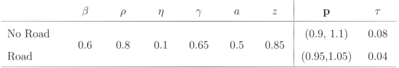
Given the numerous parameters, and corresponding degree of under-identification, there is no call for great precision everywhere. Let γ = 0.65 and the social norms demand β = 0.6 and ρ= 0.8. Households are still rather poor, so their taste for good

1 should be at least as strong as that for good 2: accordingly, let a = 0.5. Without loss of generality, set the prices of both goods in the town at unity in all periods. A survey of 30 villages in upland Orissa for the year 2009-10 (Bell and van Dillen, 2012) yields the finding that in the absence of an all-weather road, the unit transport costs for paddy, the main crop, were a bit less than 0.1, but those for other commercial crops somewhat higher. Applying the same to fertilizers, seeds and other goods bought in, households in such villages then face the price vector p_t= (0.9,1.1)∀t. As for the trip to school, the great majority of India’s villages have a primary one of their own; but only a small minority have a secondary or high school, and in the absence of an all- weather road, the daily round-trip time can be rather long. The averages for primary and secondary school pupils in the Orissa villages lacking such a road were 23 and 76 minutes, respectively. Allowing, say, twelve hours for sleeping, eating and bathing at home, and taking into account the higher opportunity costs of older children’s time, let τ = 0.08. The direct costs of state schooling are surely modest: recalling (8), let σ_t be 0.15 times the opportunity cost factor p_1tα_t(1 +τ)γ, whereby α_t has yet to be determined. For the moment, we also defer discussion of the inter-temporal taste parameters b₁ and b₂.

Coming by estimates of premature adult mortality is a far easier task than that of morbidity. In a setting of three overlapping generations, each generation corresponds to about 20 years, the age at which full adulthood is attained. The rate q_t therefore corresponds to ₂₀q₂₀, the probability that an individual will die before reaching 40, conditional on reaching 20. For India in 2005, WHO (2007) gives ₂₀q₂₀ = 0.065 and

30q₂₀ = 0.123. Something closer to the latter is suited to our present purposes, first, to allow for some mortality in the first part of old age, which the rigid time structure of the model rules out, and secondly, to reflect higher mortality among rural middle-aged adults than the all-India average. Hence, let q₁ = 0.125. If history and international experience are any guides, this is sure to fall over the coming generation, PMGSY or no.

It does not seem too much to hope that India will do as well then as China does now, so let q₂ = 0.053. Where morbidity and disability are concerned, school-age children typically suffer less sickness than their parents, who, in turn, are in better health than their aged parents. The findings from the Orissa survey confirm as much, the average number of days of reported sickness being 5.6 a year, though the contribution of chronic ailments may not have been properly covered. It is also possible that sickness was interpreted as being too unwell to go about the usual daily business at all, as opposed to being in a state of diminished capacity to do so. Thus, the vector d₁ = (0.02,0.04,0.08) represents a rather speculative stab at an estimate for period 1. Since

it is easier to ward off premature death than morbidity, the associated improvement to d₂ = (0.015,0.03,0.06) in period 2 is a bit less dramatic than that in mortality.

3.3 Setting up the sequence under perfect foresight

The system must be set up in such a way that it satisfies two requirements. First, the household must choose a plan that is in keeping with what we observe in the present. The key variable here is the level of investment in education, e₁. Children in India’s rural areas typically start school at 6 years of age and complete about 6 years of schooling on average. Hence, with up to 12 years of schooling available, and noting that morbidity reduces the endowment of productive time, the model must be set up so as to yield (1 +τ)e⁰₁ = (6/12)(1−d¹₁). A further adjustment is needed for the number of days lost due to bad weather, especially in the monsoon. The Orissa survey yields an estimated 8.6 and 9.4 days a year, on average, for primary- and secondary- school children, respectively, involuntary absences that were mainly attributable to their teachers’ failure to arrive (Bell and van Dillen, 2011). Assuming a school year of 180 days, the required condition becomes (1 +τ)e⁰₁ = (1−9/180)(6/12)(1−d¹₁) = (19/40)(1−d¹₁), where τ = 0.08 andd¹₁= 0.02.

Secondly, the whole sequence must be anchored to some plausible configuration in the future. In this connection, there is much talk of meeting the so-called Millennium Development Goals by 2015, and suchlike. Let us suppose, therefore, that a full ed- ucation for all is attainable within one complete generation, where the definition of a

‘full education’ must make a full allowance for the claims on a child’s time made by illness, traveling to school and other involuntary absences. That is to say, the model must be set up such that parents in period 2 do choose e⁰₂ = ¯e₂ = 0.95(1−d¹₂)/(1 +τ).

If the general environment described by Z_t does not deteriorate thereafter, it will then follow that e⁰_t = ¯e_t = 0.95(1−d¹_t)/(1 +τ) ∀t ≥ 3. For once e⁰_t = 0.95(1−d¹_t)/(1 +τ) is attained, the young adults in that period can then be certain that all future gen- erations will continue this policy, with its corresponding effects on their consumption in old age, as formulated in (15). The desired anchoring of the system will have been accomplished.

The simplest way of ensuring all this where Z_t is concerned is to impose stationarity from period 2 onwards. On the assumption that fertility will fall to replacement levels by 2030, and allowing for premature mortality among adults, letN_t= (2,2,1.5)∀t ≥2.

Also stationary are prices, tastes and costs, a road being built, if at all, at the start

of period 1 (see below). Recalling the discussion of mortality and morbidity in Section 3.2, we also have q_t= 0.053 and d_t= (0.015,0.03,0.06)∀t≥2.

The final step is to choose the productivity parametersz_tandαand the intertemporal taste parametersb₁ andb₂so as to yielde⁰₂ = 0.95(1−0.015)/1.08 = 0.866 with as little to spare as possible. With the exception of z_t, this must be accomplished by trial and error as part of the process of computation. The only prior restriction is that with pure impatience for consumption, b₁ > b₂. Since premature mortality already appears in connection with preferences over dated consumption, the pure discount rate arguably should not greatly exceed 15 percent per generation of 20 years.

One can arrive at an appropriate value of z by imposing the assumption that indi- vidual productivity, λ_t, will grow without limit if, after some point, all generations are fully educated. As noted in Section 2.1, by choosing a sufficiently productive technology f(e_t) and otherwise setting up the system so that e⁰_t = ¯e_t∀t≥2, where e⁰_t = ¯e_t is suf- ficiently close to 1, we ensure that λ²_t will indeed grow without bound. Recall from (3) that the relevant characteristic root when the upper limit one_tis unity is 1+g^∗. Reduc- ing this upper limit to ¯e= 0.866 yields the roota₂[1 +

(1 + 2a₃/a²₂f(0.866))]f(0.866), where f(e_t) = z_te_t, a₂ = 2/3.5 and a₃ = 1.5/3.5. Let z_t = 0.85∀t, which implies that output per head will grow at the rate of 41.3 percent per generation, or 1.74 percent a year. This seems defensible for an horizon many generations off.

4 A New Road: Exact Welfare Measures

Imagine two islands, each inhabited by a representative extended family. The first is characterized by the constellation of numerical values set out in Section 3. The second is identical, except for the happy event that a road is provided free of charge at the very start of period 1. As a result, unit transport costs, travel-times, morbidity and mortality all become lower than those on island 1. In this more benign environment, it is not only certain that e⁰_t >0.866∀t ≥2, but also highly likely thate⁰₁ will be higher than on island 1. The latter being so, the path {λ²_t}^∞_t=2 will lie everywhere above its counterpart on island 1. The two paths will, moreover, exhibit different asymptotic rates of growth, even though they share the common value of z_t. This ‘growth-effect’

stems from lower morbidity, reduced round-trip times to school and fewer involuntary absences, all of which bring the upper limit ¯e_tcloser to unity – as long as the road does not fall into utter disrepair. If it were to do so at the end of period 1, for example, e⁰_t = 0.866∀t ≥2 would still be ensured thereafter, under the hypothesis that it holds

on island 1, which will have no road in any period. Even in the face of such neglect, therefore, there would remain a ‘level-effect’.

Island 1, therefore, provides the benchmark for the following thought-experiment.

At the very start of period 1, the inhabitants of island 2 are given the choice between having the road and making do with the conditions ruling on island 1, but receiving a lump-sum payment instead. If the latter sum is such that they are indifferent between these two alternatives, we will have found the equivalent variation (EV) corresponding to the provision of the road, as assessed by the young adults in period 1 on both islands.

The road will, of course, yield further benefits in later periods, even if it falls into utter disrepair at the end of period 1. For the level-effect alluded to above will come into play, and to the associated increase in the family’s full income there will correspond an EV for that generation of young adults. In what follows, however, we will confine our attention to the EV for young adults in periods 1 and 2, leaving the task of estimating the whole sequence thereof to another paper.

4.1 The benchmark: No road

Recalling Section 3.3, the task here is to choose α, b₁ and b₂ so that e⁰₂ = 0.866 is barely attained. It is easily seen that the whole sequence {λ²_t}^∞_t=1 can be derived on the hypothesis that e⁰_t = 0.866 ∀t ≥ 2 without any reference to α, b₁ and b₂. The parameter values, the initial conditions and (25) yield

λ²₂ = 2×0.85·(19/40)(1−0.02)

1.08 · 2×1.7 + 0.75×1.2

2 + 0.75 + 1 = 2.1457. Continued recursion using {N_t}^∞_t=2 yields

λ²₃ = 2×0.85×0.866·2×2.1457 + 1.5×1.7

2 + 1.5 + 1 = 3.8791, λ²₄ = 2×0.85×0.866· 2×3.8791 + 1.5×2.1457

2 + 1.5 + 1 = 5.6195, and so forth.

Having thus determined that λ²₂ = 2.1457, the hypothesis e⁰₂ = 0.866 leaves the household in period 1 with almost all the information needed to derive p₂ ·x⁰₂ from (5), whereupon x⁰₂ would follow from the assumption that the sub-utility function u is (transformed) Cobb-Douglas. The missing element is the value of α. Moving back to calibration, therefore, it follows that by hazarding a guess at α, we are then left to

find a pair (b₁, b₂), with b₂ ≈0.85b₁, such that the solution to problem (15) in period 1 indeed involves e⁰₁ = (19/20)(6/12)(1−0.02)/1.08, whereby α may be varied until the desired result is obtained. Mindful of the need to fulfill the hypothesis e⁰₂ = 0.866, but not too comfortably, some experimenting yielded α = 5, albeit with quite strong impatience (b₂ = 0.8b₁ = 21.8047) and modest curvature of the sub-utility function φ (η= 0.1).

The resulting sequence of the main endogenous variables when there is no road is set out in the upper panel of Table 1. Three generations on, in some 60 years, a young adult is over three times more productive and enjoys a level of real consumption likewise three times higher than his or her great-grandparents were in young adulthood in period 1.

Table 1: The sequences of the main variables, with and without the road

Period 1 2 3 4

No Road x_1t 2.8177 3.6598 5.9275 9.2346

x_2t 2.3054 2.9943 4.8495 7.5556

e⁰_t 0.4310 0.8664 0.8664 0.8664

λ²_t 1.7000 2.1457 3.8791 5.6195

Road: Variant 1 x_1t 2.7605 3.8022 6.4384 10.4149

x_2t 2.4976 3.4401 5.8252 9.4230

e⁰_t 0.4907 0.9366 0.9366 0.9366

λ²_t 1.7000 2.3044 4.2567 6.4454

Road: Variant 2 x_1t 2.7537 3.8173 6.4631 10.4478

x_2t 2.4914 3.4538 5.8476 9.4527

e⁰_t 0.4959 0.9366 0.9366 0.9366

λ²_t 1.7000 2.3182 4.2692 6.4661

Variant 1: q₁ = 0.125, q_t= 0.053∀t ≥2. Variant 2: q₁ = 0.101625, q_t= 0.0451∀t≥2.

4.2 Life with the road

We need to specify how the road improves the household’s environment in period 1, as described by the vector Z₁. Starting with unit transport costs for goods, Bell and van Dillen (2012) estimate that these are reduced by about 5 percent of the net price received for commodities marketed. Khandker et al. (2009) obtain a similar estimate for rural roads in Bangladesh, once an allowance is made for greater volumes marketed.

They also estimate that the farm-gate price of fertilizers declined by 5 percent. With a new road, therefore, let p₁ = (0.95,1.05). Where schooling is concerned, Bell and van Dillen’s (2012) analysis of the Orissa survey yields substantial savings in travel-time for secondary-school pupils (just over 30 minutes a day) and far fewer days of involuntary absences for all grades (about 2 instead of about 9 for primary and 14 for secondary).

These estimates implyτ = 0.04 and ¯e_t= (1−2/180)(1−d¹_t)/(1+0.04) = 0.9508(1−d¹_t).

It is not to be expected that the provision of an all-weather road will have such strong effects on morbidity, at least in the very short run; and Bell and van Dillen (2012) find none in the Orissa villages. Households did, however, respond by switching away from local healers, quacks and primary clinics to hospitals, which certainly suggests that all-weather roads are valued in this connection. To be quite conservative, therefore, let there be no improvement ind_t ∀t. The findings where mortality is concerned are mixed.

An analysis of individual mortality in the sample households revealed no effects; but the respondents in the village ‘focus group’ interviews were adamant that mortality had dropped sharply, as the acutely sick and injured could be treated in good time.

According to their claims, in the group of nine such villages, the average number of such deaths had dropped from 3.25 to 0.75 annually. Even allowing for ‘unavoidable’

deaths, these claims are rather startling; for the crude mortality rate of about 10 per 1000 in the sample drawn from all 30 villages implies just 10 deaths annually in a typical village of 1000 souls. Since q_t is assumed to fall from 0.125 in period 1 to 0.053 in period 2 even with no road, let the provision of the road reduceq₁, not by the implied 25 percent or so, but rather by 10 percent, to 0.1125.

Turning to future periods, let the road be perfectly durable, thereby maintaining these more favourable prices of goods, as well as travel-times to, and involuntary ab- sences from, school indefinitely. As argued in Section 3.2, however, morbidity and mortality will surely fall over the next generation even in the absence of a road.

Staying on the conservative side, let the road continue to have no effect on morbid- ity in period 2, but let the 10 percent reduction in mortality continue to hold, so that q₂ = 0.0477. Thereafter, all these rates remain stationary. The configuration