Data Warehousing
& Data Mining
& Data Mining
Wolf-Tilo Balke Silviu Homoceanu
Institut für Informationssysteme
Technische Universität Braunschweig http://www.ifis.cs.tu-bs.de
8. Building the DW
8.1 The DW Project
8.2 Data Extract/Transform/Load (ETL) 8.3 Metadata
8. Building the DW
• Building a DW, is a complex IT project
– A middle size DW-project contains 500-1000 activities
• DW-Project organization
– Project roles and corresponding tasks, e.g.:
8.1 The DW Project
– Project roles and corresponding tasks, e.g.:
Roles Tasks
DW-PM Project Management
DW-Architect Methods, Concepts, Modeling DW-Miner Concepts, Analyze(non-standard) Domain Expert Domain Knowledge
DW-System Developer System- and metadata-management, ETL
• DW-Project usual tasks
– Communication, as process of information exchange between team members
– Conflict management
The magical triangle, compromise between time, costs and
8.1 The DW Project
• The magical triangle, compromise between time, costs and quality
– Quality assurance
• Performance, reliability, scalability, robustness, etc.
– Documentation
• Software choice
– Database system for the DW
• Usually the choice is to use the same technology provider as for the operational data
• MDB vs. RDB
– ETL tools
8.1 The DW Project
– ETL tools
• Differentiate by the data cleansing needs
– Analysis tools
• Varying from data mining to OLAP products, with a focus on reporting functionality
– Repository
• Not very oft used
• Hardware choice
– Data storage
• RAID systems, SAN’s, NAS’s
– Processing
8.1 The DW Project
• Multi-CPU systems, SMP, Clusters
– Failure tolerance
• Data replication, mirroring RAID, backup strategies
– Other factors
• Data access times, transfer rates, memory bandwidth, network throughput and latency
• Project Timeline, depends on the development methodology, but usually
– Phase I – Proof of Concept
• Establish Technical Infrastructure
• Prototype Data Extraction/Transformation/Load
• Prototype Analysis & Reporting
8.1 The DW Project
• Prototype Analysis & Reporting
– Phase II – Controlled Release
• Iterative Process of Building Subject Oriented Data Marts
– Phase III – General Availability
• On going operations, support and training, maintenance and growth
• The most important part of the DW building project
is defining the ETL process
• What is ETL?
– Short for extract, transform, and load
– Three database functions that are combined into one tool to pull data out of productive databases and place it into the DW
8.2 ETL
place it into the DW
• Migrate data from one database to another, to form data marts and data warehouses
• Convert databases from one format or type to another
• When should we ETL?
– Periodically (e.g., every night, every week) or after significant events
– Refresh policy set by administrator based on user needs and traffic
8.2 ETL
needs and traffic
– Possibly different policies for different sources – Rarely, on every update (real-time DW)
• Not warranted unless warehouse data require current data (up to the minute stock quotes)
• ETL is used to integrate heterogeneous systems
– With different DBMS, operating system, hardware, communication protocols
• ETL challenges
8.2 ETL
– Getting the data from the source to target as fast as possible
– Allow recovery from failure without restarting the whole process
• This leads to balance between writing data to
• Staging area, basic rules
– Data in the staging area is owned by the ETL team
• Users are not allowed in the staging area at any time
8.2 ETL
area at any time
– Reports cannot access data from the staging area
– Only ETL processes can write to and read from the staging area
8.2 ETL
• ETL input/output example
• Staging area structures for holding data
– Flat files
– XML data sets – Relational tables
8.2 Staging area data structures
• Flat files
– ETL tools based on scripts, such as Perl, VBScript or JavaScript
– Advantages
• No overhead of maintaining metadata as DBMS does
8.2 Staging area data structures
• No overhead of maintaining metadata as DBMS does
• Sorting, merging, deleting, replacing and other data-migration functions are much faster outside the DBMS
– Disadvantages
• No concept of updating
• Queries and random access lookups are not well supported by the operating system
• When should flat files be used?
– Staging source data for safekeeping and recovery
• Best approach to restart a failed process is by having data dumped in a flat file
– Sorting data
8.2 Staging area data structures
– Sorting data
• Sorting data in a file system may be more efficient as performing it in a DBMS with Order By clause
• Sorting is important: a huge portion of the ETL processing cycles goes to sorting
• When should flat files be used?
– Filtering
• Using grep-like functionality
– Replacing text strings
8.2 Staging area data structures
• Sequential file processing is much faster at the system-level than it is with a database
• XML Data sets
– Used as common format for both input and output from the ETL
system
– Generally, not used for persistent
8.2 Staging area data structures
– Generally, not used for persistent staging
– Useful mechanisms
• XML schema (successor of DTD)
• XQuery, XPath
• XSLT
• Relational tables
– Using tables is most appropriate especially when there are no dedicated ETL tools
– Advantages
• Apparent metadata: column names data types and lengths,
8.2 Staging area data structures
• Apparent metadata: column names data types and lengths, cardinality, etc.
• Relational abilities: data integrity as well as normalized staging
• Open repository/SQL interface: easy to access by any SQL compliant tool
– Disadvantages
• How is the staging area designed?
– Staging database, file system, and directory structures are set up by the DB and OS administrators based on ETL architect estimations e.g., tables volumetric
worksheet
8.2 Staging area storage
worksheet
Table Name
Update strategy
Load frequency
ETL Job Initial row count
Avg row length
Grows with
Expected rows/mo
Expected bytes/mo
Initial table size
Table Size 6 mo. (MB) S_ACC Truncate/
Reload
Daily SAcc 39,933 27 New
account
9,983 269,548 1,078,191 2.57
S_ASSETS Insert/
Delete
Daily SAssets 771,500 75 New
assets
192,875 15,044,250 60,177,000 143.47
S_DEFECT Truncate/
Reload
On demand
SDefect 84 27 New
defect
21 567 2,268 0.01
• ETL
– Data extraction
– Data transformation – Data loading
8.2 ETL
Data loading
• Data Extraction
– Data needs to be taken from a data source so that it can be put into the DW
• Internal scripts/tools at the data source, which export the data to be used
8.2 Data Extraction
which export the data to be used
• External programs, which extract the data from the source
– If the data is exported, it is typically exported into a text file that can then be brought into an intermediary
database
– If the data is extracted from the source, it is typically transferred directly into an intermediary database
• Steps in data extraction
– Initial extraction
• Preparing the logical map
• First time data extraction
– Ongoing extraction
8.2 Data Extraction
– Ongoing extraction
• Just new data
• Changed data
• Or even deleted data
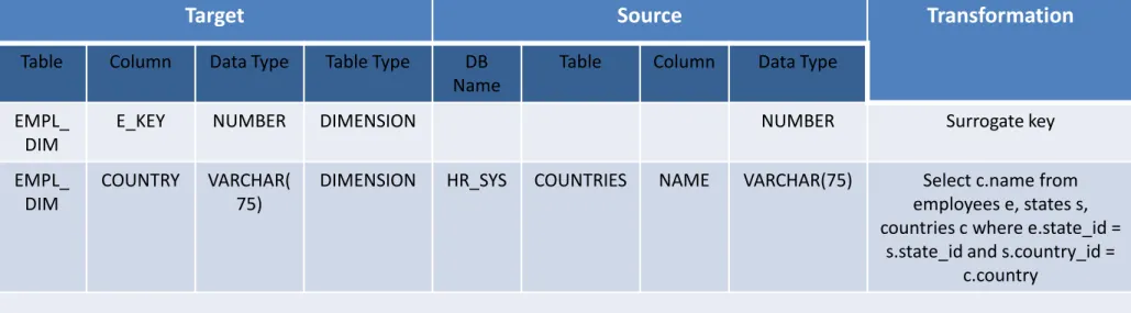
• Logical map connects the original source data to the final data
– Most important part is the description of the transformation rules
8.2 Data Extraction
Target Source Transformation
Table Column Data Type Table Type DB Name
Table Column Data Type
EMPL_
DIM
E_KEY NUMBER DIMENSION NUMBER Surrogate key
EMPL_
DIM
COUNTRY VARCHAR(
75)
DIMENSION HR_SYS COUNTRIES NAME VARCHAR(75) Select c.name from employees e, states s, countries c where e.state_id =
s.state_id and s.country_id = c.country
• Building the logical map: first identify the data sources
– Data discovery phase
• Collecting and documenting source systems: databases, tables, relations, cardinality, keys, data types, etc.
8.2 Data Extraction
tables, relations, cardinality, keys, data types, etc.
– Anomaly detection phase
• NULL values can destroy any ETL process, e.g., if a foreign key is NULL, joining tables on a NULL column results in data loss, because in RDB NULL ≠ NULL
– If NULL on foreign key then use outer joins
– If NULL on other columns then create a business rule to replace NULLs while loading data in DW
• Data needs to be maintained in the DW also after the initial load
– Extraction is performed on a regular basis
– Only changes are extracted after the first time
8.2 Ongoing Extraction
• Detecting changes (new/changed data)
– Using audit columns
– Database log scraping or sniffing – Process of elimination
8.2 Ongoing Extraction
Process of elimination
• Detecting changes (new/changed data)
– Using audit columns
• Store date and time a record has been added or modified
• Detect changes based on date stamps higher than the last extraction date
8.2 Ongoing Extraction
extraction date
– Log scraping
• Takes a snapshot of the database redo log at a certain time (e.g., midnight) and finds the transactions affecting the tables ETL is interested
• It can be problematic when the redo log
8.2 Detecting changes
• It can be problematic when the redo log gets full and is emptied by the DBA
– Log Sniffing
• Pooling the redo log capturing the transactions on the fly
• The better choice: suitable also for real-time ETL
– Process of Elimination
• Preserves exactly one copy of each previous extraction
• During next run, it compares the entire source tables against the extraction copy
• Only differences are sent to the DW
8.2 Detecting changes
• Only differences are sent to the DW
• Advantages
– Because the process makes row by row comparisons, it is impossible to miss data
– It can also detect deleted rows
• Detecting deleted or overwritten fact records
– If records or incorrect values are inserted by mistake, records in ODS get deleted or overwritten
– If the mistakes have already been loaded in the DW, corrections have to be made
8.2 Detecting changes
corrections have to be made
– In such cases the solution is not to modify or delete data in the DW, but inserting an additional record which corrects or even cancels the mistake by negating it
• Data transformation
– Uses rules or lookup tables, or creating combinations with other data, to convert source data to the desired state
• 2 major steps
8.2 Data Transformation
• 2 major steps
– Data Cleaning
• Mostly involves manual work
• Assisted by artificial intelligence algorithms and pattern recognition
– Data Integration
• Extracted data can be dirty. How does clean data look like?
• Data Quality characteristics:
– Correct: values and descriptions in data represent
8.2 Data Cleaning
– Correct: values and descriptions in data represent their associated objects truthfully
• E.g., if the city in which store 1 is located is Braunschweig, then the address should not report Paris.
– Unambiguous: the values and descriptions in data can be taken to have only one meaning
– Consistent: values and descriptions in data use one constant notational convention
• E.g., Braunschweig can be expressed as BS or Brunswick, by our employees in USA. Consistency means using just BS in all our data
8.2 Data Cleaning
all our data
– Complete
• Individual values and descriptors in data have a value (not null)
• Aggregate number of records is complete
• The data cleaning engine produces 3 main deliverables:
– Data-profiling results:
• Meta-data repository describing schema definitions, business objects, domains, data sources, table definitions, data rules,
8.2 Data Cleaning
objects, domains, data sources, table definitions, data rules, value rules, etc.
• Represents a quantitative assessment of original data sources
– Error event table
• Structured as a dimensional star schema
• Each data quality error identified by the cleaning subsystem is inserted as a
row in the error
8.2 Cleaning Deliverables
row in the error event fact table
Data Quality Screen:
- Status report on data quality
- Gateway which lets only clean data
– Audit dimension
• Describes the data-quality context of a fact table record being loaded into the DW
• Attached to each fact record
• Aggregates the information from the error event table on a
8.2 Cleaning Deliverables
• Aggregates the information from the error event table on a per record basis
Audit key (PK)
Completeness category (text) Completeness score (integer)
Number screens failed Max severity score
Extract timestamp Clean timestamp
• Core of the data cleaning engine
– Break data into atomic units
• E.g., breaking the address into street, number, city, zip and country
– Standardizing
8.2 Cleaning Engine
– Standardizing
• E.g., encoding of the sex: 0/1, M/F, m/f, male/female
– Verification
• E.g., does zip code 38106 belong to Braunschweig?
– Matching
• Types of enforcement
– Column property enforcement
• Ensures that incoming data contains expected values
• NULL values in required columns
• Numeric values outside the expected high/low ranges
8.2 Data quality checks
• Numeric values outside the expected high/low ranges
• Columns whose lengths are unexpectedly short or long
• Columns that contain values outside of valid value sets
• Adherence to a required pattern
• Hits against a list of known wrong values (if the list of acceptable values is to long)
• Structure enforcement
– Focus on the relationship of columns to each other – Proper primary and foreign keys
– Explicit and implicit hierarchies and relationships
8.2 Data quality checks
Explicit and implicit hierarchies and relationships among group of fields e.g., valid postal address
• Data and Value rule enforcement
– E.g., a commercial customer cannot simultaneously be a limited and a corporation
– Value rules can also provide probabilistic warnings that the data might be incorrect
8.2 Data quality checks
that the data might be incorrect
• E.g., boy named ‘Sue’ might be correct, but most probably it is a gender or name error and such a record should be
flagged for inspection
• Overall Process Flow
8.2 Data cleaning
• Sometimes data is just garbage
– We shouldn’t load garbage in the DW
8.2 Data Quality
• Cleaning data manually
takes just…forever!!!
• Use tools to clean data semi-automatic
– Open source tools
• E.g., Eobjects DataCleaner, Talend Open Profiler
– Non-open source
8.2 Data Quality
• Firstlogic both by Business Objects (now SAP)
• Vality both by Ascential (now IBM)
• Oracle Data Quality and Oracle Data Profiling
• Data cleaning process
– Use of regular expressions
8.2 Data Quality
• Regular expressions for date/time data
8.2 Data Quality
• Core of the data cleaning engine
– Anomaly detection phase:
• Data anomaly is a piece of data which doesn’t fit into the domain of the rest of the data it
8.2 Cleaning Engine
domain of the rest of the data it is stored with
• “What is wrong with this picture?”
• Anomaly detection
– Count the rows in a table while grouping on the column in question e.g.,
• SELECT city, count(*) FROM order_detail GROUP BY city
8.2 Anomaly detection
City Count(*)
Bremen 2
Berlin 3
WOB 4,500
BS 12,000
HAN 46,000
…
• What if our table has 100 million rows with 250,000 distinct values?
– Use data sampling e.g.,
• Divide the whole data into 1000 pieces, and choose 1 record from each
8.2 Anomaly detection
record from each
• Add a random number column to the data, sort it an take the first 1000 records
• Etc.
– Common mistake is to select a range of dates
• Most anomalies happen temporarily
• Data profiling
– E.g., observe name anomalies
8.2 Data Quality
• Data profiling
– Pay closer look to strange values – Observe data distribution pattern
• Gaussian distribution
8.2 Data Quality
SELECT AVERAGE(sales_value) – 3 * STDDEV(sales_value), AVERAGE(sales_value) + 3 * STDDEV(sales_value) INTO Min_resonable, Max_resonable FROM …
• Data distribution
– Flat distribution
• Identifiers distributions (keys)
– Zipfian distribution
8.2 Data Quality
• Word ranking by frequency
• Web page hits follow this distribution
– Home page many hits
• Some values appear more often than others
– In sales, more cheap goods are sold than expensive ones
• Data distribution
– Pareto, Poisson, S distribution
• Distribution Discovery
– Statistical software: SPSS, StatSoft, R, etc.
8.2 Data Quality
– Statistical software: SPSS, StatSoft, R, etc.
• Data integration
– Several conceptual schemas need to be combined into a unified global schema
– All differences in perspective and terminology have to be resolved
8.2 Data Integration
terminology have to be resolved – All redundancy has to be
removed
schema 2
schema schema 4 schema 3
schema 3 schema 1 schema 1
• There are four basic steps needed for conceptual schema integration
1. Preintegration analysis 2. Comparison of schemas 3. Conformation of schemas
8.2 Schema integration
3. Conformation of schemas 4. Merging and restructuring
of schemas
• The integration process needs continual refinement and
reevaluation
8.2 Schema integration
schemas with conflicts
list of conflicts
identify conflicts
Preintegration analysis Comparison of schemas
modified schemas
integrated
resolve conflicts
integrate schemas
Conformation of schemas
Merging and restructuring
• Preintegration analysis needs a close look on the individual conceptual schemas to decide for an adequate integration strategy
– The larger the number of constructs, the more important is modularization
8.2 Schema integration
more important is modularization – Is it really sensible/possible
to integrate all schemas?
8.2 Schema integration
Integration strategy
Binary approach n-ary approach
Sequential Balanced
integration
One-shot integration
Iterative integration
• Schema conflicts
– Table/Table conflicts
• Table naming e.g., synonyms, homonyms
• Structure conflicts e.g., missing attributes
• Conflicting integrity conditions
8.2 Schema integration
• Conflicting integrity conditions
– Attribute/Attribute conflicts
• Naming e.g., synonyms, homonyms
• Default value conflicts
• Conflicting integrity conditions e.g., different data types or boundary limitations
– Table/Attribute conflicts
• The basic goal is to make schemas compatible for integration
• Conformation usually needs manual interaction
– Conflicts need to be resolved semantically
8.2 Schema integration
– Conflicts need to be resolved semantically – Rename entities/attributes
– Convert differing types, e.g., convert an entity to an attribute or a relationship
– Align cardinalities/functionalities – Align different datatypes
• Schema integration is a semantic process
– This usually means a lot of manual work
– Computers can support the process by matching some (parts of) schemas
8.2 Schema integration
• There have been some approaches towards (semi-)automatic matching of schemas
– Matching is a complex process and usually only
focuses on simple constructs like ‘Are two entities semantically equivalent?’
• Schema Matching
– Label-based matching
• For each label in one schema consider all labels of the other schema and every time gauge their semantic similarity
– Instance-based matching
• Looking at the instances (of entities or relationships) one can e.g.,
8.2 Schema integration
• Looking at the instances (of entities or relationships) one can e.g., find correlations between attributes like ‘Are there duplicate
tuples?’ or ‘Are the data distributions in their respective domains similar?’
– Structure-based matching
• Abstracting from the actual labels, only the structure of the schema is evaluated, e.g., regarding element types, depths in hierarchies, number and type of relationships, etc.
• If integration is query-driven only Schema Mapping is needed
– Mapping from one or more source schemas to a target schema
8.2 Schema integration
High-level mapping
Data Source schema S
Correspondence
Target schema T
Correspondence
Mapping compiler
Low-level mapping High-level mapping
• Schema Mapping
– Abstracting from the actual labels, regarding element types, depths in hierarchies, number and type of
relationships, etc.
8.2 Schema integration
Product
ProdID: Decimal Product: VARCHAR(50)
Group: VARCHAR(50) Categ: VARCHAR(50) Product
ID: Decimal Product: VARCHAR(50)
GroupID:Decimal
• Schema mapping automation
– Complex problem, based on heuristics – Idea:
• Based on given schemas and a high level mapping between them
8.2 Schema integration
them
• Generate a set of queries that transform and integrate data from the sources to conform to the target schema
– Problems
• Generation of the correct query considering the schemas and the mappings
• Guarantee that the transformed data correspond to the target schema
• Schema integration in praxis
– BEA AquaLogic Data Services
• Special Feature: easy-to-use modeling: “Mappings and transformations can be designed in an easy-to-use GUI tool using a library of over 200 functions. For
8.2 Schema integration
www.bea.com
tool using a library of over 200 functions. For complex mappings and
transformations, architects and developers can bypass the GUI tool and use an Xquery source code editor to define or edit services. “
• What tools are actually given to support integration?
– Data Translation Tool
• Transforms binary data into XML
• Transforms XML to binary data
8.2 Schema integration
• Transforms XML to binary data
– Data Transformation Tool
• Transforms an XML to another XML
– Base Idea
• Transform data to application specific XML →Transform to XML specific to other application / general schema →
Transform back to binary
• “I can’t afford expensive BEA consultants and the AquaLogic Integration Suite, what now??”
– Do it completely yourself
• Most used technologies can be found as Open Source projects (data mappers, XSL engines, XSL editors, etc)
8.2 Schema integration
projects (data mappers, XSL engines, XSL editors, etc)
– Do it yourself with specialized tools
• Many companies and open source projects are specialized in developing data integration and transformation tools
– CloverETL
– Altova MapForce
– BusinessObjects Data Integrator – etc…
• Altova MapForce
– Same idea than BEA Integrator
• Also based on XSLT and a data description language
– Editors for binary/DB to XML mapping
8.2 Schema integration
XML mapping – Editor for XSL
transformation
– Automatic generation of data sources, web- services, and
transformation modules in Java, C#, C++
• The loading process can be broken down into 2 different types:
– Initial load
– Continuous load (loading over time)
8.2 Loading
over time)
• Issues
– Huge volumes of data to be loaded
– Small time window available when warehouse can be taken off line (usually nights)
8.2 Loading
– When to build index and summary tables
– Allow system administrators to monitor, cancel, resume, change load rates
– Recover gracefully -- restart after failure from where you were and without loss of data integrity
• Initial Load
– Deliver dimensions tables
• Create and assign surrogate keys, each time a new cleaned and conformed dimension record has to be loaded
• Write dimensions to disk as physical tables, in the proper dimensional format
8.2 Loading
dimensional format
– Deliver fact tables
• Utilize bulk-load utilities
• Load in parallel
– Tools
• DTS – Data Transformation Services
• bcp utility – batch copy
• Continuous load (loading over time)
– Must be scheduled and processed in a specific order to maintain integrity, completeness, and a satisfactory level of trust
– Should be the most carefully planned step in data
8.2 Loading
– Should be the most carefully planned step in data warehousing or can lead to:
• Error duplication
• Exaggeration of inconsistencies in data
• Continuous load of facts
– Separate updates from inserts
– Drop any indexes not required to support updates – Load updates
8.2 Loading
Load updates
– Drop all remaining indexes
– Load inserts through bulk loaders – Rebuild indexes
• Metadata - data about data
– In DW, metadata describe the contents of a data warehouse and how to use it
• What information exists in a data warehouse, what the information means, how it was derived, from what source
8.3 Metadata
information means, how it was derived, from what source systems it comes, when it was created, what pre-built
reports and analyses exist for manipulating the information, etc.
• Types of metadata in DW
– Source system metadata – Data staging metadata – DBMS metadata
8.3 Metadata
• Source system metadata
– Source specifications
• E.g., repositories, and source logical schemas
– Source descriptive information
8.3 Metadata
• E.g., ownership descriptions, update frequencies and access methods
– Process information
• E.g., job schedules and extraction code
• Data staging metadata
– Data acquisition information, such as data
transmission scheduling and results, and file usage – Dimension table management, such as definitions of
dimensions, and surrogate key assignments
8.3 Metadata
dimensions, and surrogate key assignments – Transformation and aggregation, such as data
enhancement and mapping, DBMS load scripts, and aggregate definitions
– Audit, job logs and documentation, such as data lineage records, data transform logs
– E.g., Cube description metadata
8.3 Metadata
• Business Intelligence (BI)
– Principles of Data Mining – Association Rule Mining