Colloidal Microswimmers driven by Thermophoresis

(1)

Colloidal Microswimmers driven by Thermophoresis

Inaugural-Dissertation

Erlangung des Doktorgrades zur

der Mathematisch-Naturwissenschaftlichen Fakultät der Universität zu Köln

vorgelegt von

Martin Wagner aus Düsseldorf

Köln 2017

(2)

Berichterstatter: Prof. Dr. Gerhard Gompper (Gutachter) Prof. Dr. Ulrich K. Deiters

Dr. Marisol Ripoll

Tag der mündlichen Prüfung: 8. November 2017

(3)

Abstract

Synthetic colloidal microswimmers have received increasing scientific interest over the past years due to their potential applications in micro-fluidics and medicine.

The dynamics of such swimmers depend on many factors such as confinement, hydrodynamics, surface interactions, or external fields. The driving mechanism of phoretic colloidal swimmers is based on an asymmetric structure. One part of the swimmer will steadily produce a local gradient (temperature, concentration, or charge) in the surrounding fluid. A different part of the swimmer will be exposed to that gradient, decaying along its surface, and thereby experiences a phoretic driving force. Since many effects are simultaneously present in real-world applications, computer simulations offer a versatile tool to understand the dynamics of microswimmers, especially through the possibility of turning specific interactions or effects off and hence understanding how they affect the behavior.

In this thesis, thermal microswimmers, especially those with a dimeric type of construction, are studied using a mesoscopic computer simulation method, multi- particle collision dynamics, which correctly describes the major features required for thermophoresis, i.e. heat transport and hydrodynamics. After a general introduction to the subject matter and methods, the general microscopic, hydrodynamic framework of phoretic effects is extended to model colloidal thermophoresis as the combined effect of a temperature and corresponding density gradient, with application to single colloid thermophoresis. The obtained results match simulation measurements well and make it possible to easily predict the response of colloids modeled with arbitrary interactions to a temperature gradient. Single swimmer dynamics are studied for two reference models, the Janus particle and the dimer type of construction. Their construction parameters determine their behavior, both in terms of propulsion velocity as well as hydrodynamic flow fields. The latter may qualitatively change, especially in case of the dimer which shows a prominent change between lateral hydrodynamic repulsion and attraction as a function of its geometric construction. Pairs of dimers are studied as well, showing a variety of depletion-induced bound states. Comparison between chemically and thermally driven swimmers shows their qualitative behavior to not depend on the phoretic mechanism employed for propulsion, neither for single swimmers nor pairs. An examination of depletion interactions is undertaken, which arise as a simulation ar- tifact in the simulation method. On this basis, parameters are chosen to physically correct employ the simulation method in the context of many-particle systems, without spurious depletion interactions. Ensembles of thermophoretic dimers are studied in large-scale simulations. Phoretic attraction is shown to lead to crystal- lization dynamics, with microswimmers forming large and long-time stable, ordered

(4)

aggregates. In case of phoretic repulsion, when combined with hydrodynamic lateral attraction stemming from the choice of appropriate construction parameters, a unique kind of dynamic, front-like swarming behavior emerges at intermediate swimmer densities. This phenomenology may offer more versatility and new possibilities in the design of applications based on active matter systems.

(5)

Kurzzusammenfassung

Aufgrund ihrer vielfältigen möglichen Anwendungspotentiale in Bereichen wie Mi- krofluidik und Medizin haben synthetische, kolloidale Mikroschwimmer in den letz- ten Jahren an wissenschaftlicher Bedeutung gewonnen. Das Verhalten dieser Schwim- mer hängt von vielen Faktoren ab, unter anderem von ihren spezifischen Oberflä- chenwechselwirkungen, ihrem hydrodynamischem Verhalten, räumlicher Beschrän- kung und eventuellen externen Feldern. Der Antriebsmechanismus phoretischer kol- loidaler Schwimmer basiert auf ihrer asymmetrischen Struktur. Ein Teil des Kollo- ids produziert stetig einen lokalen (Temperatur-, Konzentrations- oder elektrischen) Gradienten in der umgebenden Flüssigkeit. Ein anderer Teil des Kolloids ist die- sem Gradienten ausgesetzt und erfährt hierdurch eine phoretische Kraft, die den Schwimmer antreibt. Aufgrund der Komplexität dieser Systeme bieten sich Compu- tersimulationen als geeignete Methode an, um die Dynamik von Mikroschwimmern zu untersuchen und zu verstehen, insbesondere da einzelne physikalische Wechsel- wirkungen kontrolliert zu- und abgeschaltet werden können, was eine Abschätzung ihres spezifischen Einflusses auf das System ermöglicht.

Die vorliegende Arbeit beschäftigt sich mit thermischen Mikroschwimmern, insbesondere einer Dimer-artigen Konstruktion. Zur Untersuchung wird die meso- skopische Simulationsmethode multi-particle collision dynamics benutzt, die die für Thermophorese notwendigen physikalischen Prozesse, vornehmlich Hydrodyna- mik und Wärmetransport, korrekt beschreibt. Nach einer allgemeinen Einführung in Thema und Methoden wird eine Erweiterung der grundlegenden Beschreibung phoretischer Effekte auf Thermophorese vorgestellt, in deren Rahmen der thermo- phoretische Effekt als Kombination der Einflüsse eines Temperaturgradienten und des daraus resultierenden Dichtegradienten interpretiert wird. Diese Beschreibung wird im Rahmen der Thermophorese einzelner Kolloide getestet und zeigt gute Übereinstimmung mit Simulationsergebnissen. Sie ermöglicht eine leichte Vorher- sage der Reaktion durch beliebige Wechselwirkungspotentiale modellierter Kolloide auf einen Temperaturgradienten. Die Dynamik einzelner Mikroschwimmer wird für die Referenzmodelle der Janus- und der Dimer-Konstruktion untersucht. Neben der Antriebsgeschwindigkeit zeigt deren geometrische Konstruktion entscheiden- den Einfluss auf ihre hydrodynamischen Strömungsfelder. Letztere können sich als Funktion der geometrischen Konstruktion des Schwimmers qualitativ ändern, insbesondere im Sinne eines ausgeprägten Wechsels von lateraler Anziehung zu Ab- stoßung im Falle des Dimers. Die Untersuchung von Paaren von Dimeren zeigt die Bildung einiger gebundener Zustände auf, die durchdepletion-Wechselwirkungen in- duziert werden. Der Vergleich zu chemisch angetriebenen Mikroschwimmern zeigt, dass das qualitative Verhalten phoretischer Mikroschwimmer nicht von der Art

(6)

des phoretischen Antriebs abhängt. Die depletion-Wechselwirkung tritt artifiziell in mesoskopischen Simulationen auf. Eine genauere Untersuchung ermöglicht es, durch Auswahl geeigneter Parameter Mikroschwimmer ohnedepletion zu modellie- ren. Darauf aufbauend wird der Fall großer Systeme von Dimeren untersucht. Im Falle phoretischer Anziehung stellt ebendiese den wesentlichsten Einfluss auf die Dynamik der Schwimmer dar und führt zur Bildung stabiler, kristalliner Struktu- ren. Der entgegengesetzte Fall phoretischer Abstoßung resultiert, im Zusammen- spiel mit lateraler hydrodynamischer Anziehung und bei mittleren Dichten, in der Bildung einzigartiger Schwärme von Dimeren mit ausgeprägter Tendenz zur geord- neten Bewegung in planaren Schichten. Dieses Schicht-artige Schwarmverhalten von Kolloiden hat Anwendungspotential in Bereichen der weichen Materie und könnte dort neue Konstruktionsmöglichkeiten eröffnen.

(7)

List of Figures

1.1 Microscope images of several biological microswimmers. . . 1

1.2 Several examples of collective motion of micro- and macroorganisms. 2 1.3 Examples of artificial microswimmers. . . 4

1.4 Examples of dimeric microswimmers. . . 5

1.5 Experimental results on the Soret coefficient. . . 13

2.1 Schematics showing the MPC algorithm. . . 19

2.2 Scaling results of the MPC-MD implementation. . . 25

3.1 Local coordinate system attached to the colloidal surface. . . 28

3.2 Fluid temperature and density distribution in the scenario of thermal gradients. . . 32

3.3 Flow field and backflow of a fixed colloid in a temperature gradient. 36 3.4 Temperature dependence of the Soret coefficient. . . 43

3.5 Analysis of conributions to the slip velocity. . . 43

3.6 Size dependence of the Soret coefficient for hard spheres with radius B. . . 45

4.1 Snapshots of synthesized dimers. . . 47

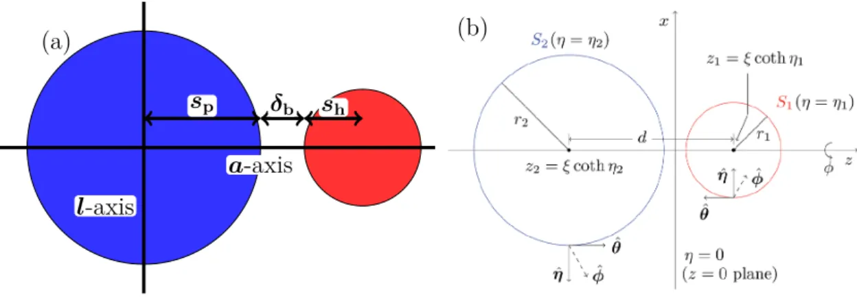
4.2 Schematic of a dimer and corresponding bispherical coordinate system. 49 4.3 Finite size effect on the propulsion velocity of a dimer swimmer. . . 54

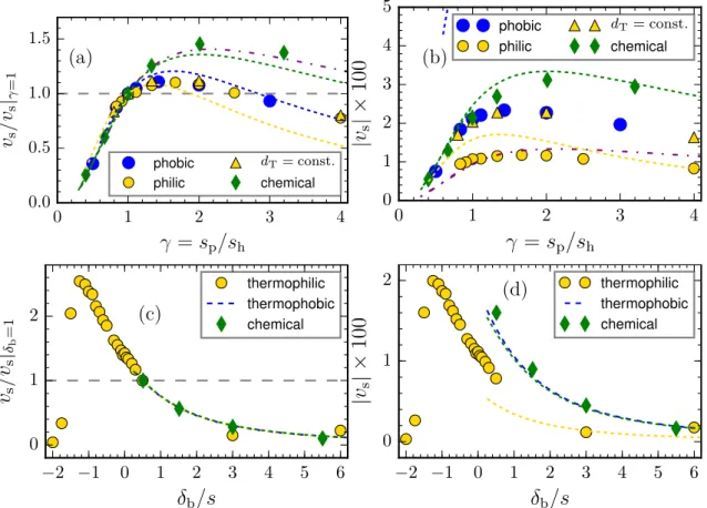
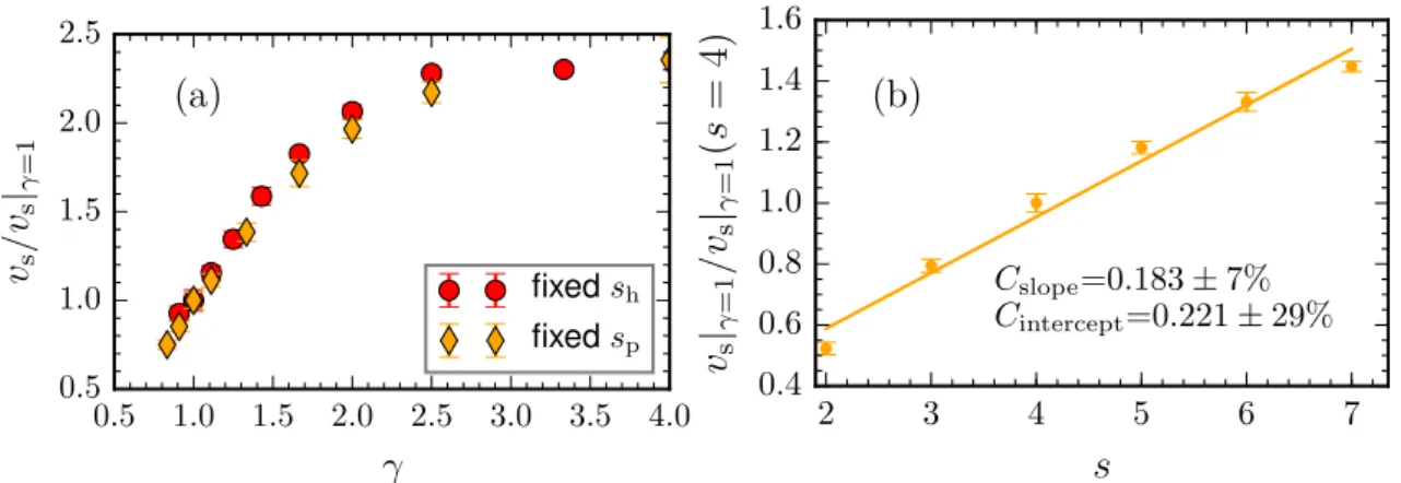
4.4 Dimer swimming velocities as a function of geometric construction. 56 4.5 Dimer propulsion velocity as a function ofγ when the size of the hot bead is fixed and size dependence of the symmetric dimer’s velocity. 58 4.6 Flow fields of thermally driven dimers. . . 60

4.7 Flow field characterization for thermophobic dimers. . . 62

4.8 Propulsion velocities and flow fields of a thermally driven Janus colloid and their dependence on the coating angle. . . 67

5.1 Schematic of quantitative descriptors for bound states of two dimers. 72 5.2 Bound states of thermophilic dimers. . . 73

5.3 Bound states of thermophobic dimers. . . 73

5.4 Structural features of the Brownian Pair bound states. . . 74

5.5 Structural features of the Moving Pair and Swimming-Together Pair bound states. . . 75

5.6 Structural features of the Rotating Pair and Reverse Brownian Pair bound states. . . 75

5.7 Phase diagrams for bound state formation of pairs of dimers. . . 76

(12)

List of Figures

6.1 Depletion-induced clustering of polystyrene spheres. . . 81

6.2 Sketch of depletion mechanism. . . 82

6.3 Depletion forces for different simulation parameters. . . 85

6.4 Examples of depletion potentials. . . 88

6.5 Depletion forces when displacements are used. . . 89

7.1 Structures of ensembles of self-propelled rods. . . 92

7.2 Influence of displacements on dimer properties. . . 94

7.3 Flow fields of thermally driven dimers used in simulations of bigger ensembles. . . 96

7.4 Snapshots of ensembles of thermophilic dimers. . . 100

7.5 Properties of ensembles of thermophilic dimers. . . 102

7.6 Bigger ensemble of thermophilic dimers. . . 104

7.7 Snapshots of ensembles of thermophobic dimers. . . 105

7.8 Cluster properties of ensembles of thermophobic dimers. . . 106

7.9 Snapshots of swarms of asymmetric thermophobic dimers. . . 108

7.10 Structural features of collectives of thermophobic dimers. . . 109

7.11 Percolated formation of asymmetric dimers. . . 111

7.12 Cluster properties of ensembles of asymmetric thermophobic dimers at different volume fractions. . . 113

7.13 Phase diagram of thermophobic dimers. . . 114

7.14 Snapshots of ensembles of depleted thermophobic dimers. . . 116

7.15 Cluster properties of ensembles of asymmetric, depleted, thermophobic dimers. . . 117

vi

(13)

List of Tables

2.1 Analytic predicitions for MPC fluid properties. . . 22 3.1 Theoretical and simulation results on the thermal diffusion factor. . 35 3.2 Theoretical and simulation results on the size dependence of the

thermal diffusion factor. . . 40 7.1 Single dimer properties for the two reference constructions of ther-

mophobic and thermophilic dimers. . . 97

(14)

(15)

Acronyms

AO Asakura-Oosawa. 82 BD Brownian Dynamics. 18 BP Brownian Pair. 72–74, 77, 78 IP Independent Pair. 72, 73, 77

LD Langevin Dynamics. 18, 98, 99, 102, 103, 106, 107, 109, 110, 113, 115, 119 LJ Lennard-Jones. 17

MD Molecular Dynamics. 15, 16, 18, 22, 24, 25

MIPS Motility-Induced Phase Separation. 2, 64, 91, 93, 118 MP Moving Pair. 72–75, 77, 78

MPC Multi-Particle Collision Dynamics. 15, 19–25, 30–32, 36, 39, 64, 65, 71, 83–86, 98, 119

MPC-MD Multi-Particle Collision Dynamics coupled to Molecular Dynamics. 22, 24, 25, 30, 31, 34, 45, 46, 48, 68, 71, 78, 79, 81, 83–85, 90, 93, 98, 99, 102, 103, 106, 107, 109, 110, 112, 114–116, 119–122

MSD Mean Squared Displacement. 7, 95 RBP Reverse Brownian Pair. 73–75, 77 RP Rotating Pair. 73–75, 77

SPTA Single-Particle Thermal Diffusion Algorithm. 34–36, 44 ST Swimming-Together Pair. 73–75, 77, 78, 122

WCA Weeks-Chandler-Andersen. 17, 18, 87, 89

(16)

(17)

Symbols

ω Angular velocity

kB Boltzmann constant

B Boundary layer width

c Concentration

ρ Density

D Diffusion coefficient

d Dimensionality

γ Dimer bead size ratio

δ_b Dimer bond length parameter

r Distance

µ_d Dynamic viscosity

Ξ Eigenvalue of gyration tensor

W External potential

δ Extra separation distance

G Fluctuation strength

D_f Fluid diffusion coefficient

ζ Fluid friction coefficient

J Flux

f,f, F,F Force

q Heat flux

I Identity matrix

U Interaction potential

r_c Interaction potential cutoff

∆ Interaction potential displacement

s Interaction potential effective range

n Interaction potential exponent

σ Interaction potential range parameter

C Interaction potential shift parameter

ε Interaction potential strength parameter

θ_c Janus coating angle

ν Kinematic viscosity

Ma Mach number

m, M Mass

µ Mobility

p Momentum exchange

Ψ MPC Bin

(18)

Symbols

a MPC cell side length

h MPC collision time

α MPC rotation angle

R MPC rotation matrix

n_ρ Number density

N Number of swimmers

e Orientation

Pe Peclet number

r,R Position vector

E Potential energy

Pr Prandtl number

p Pressure

P Probability density

R Radius

ξ Random force

τ Relaxation time

r/a repulsive/attractive

Re Reynolds number

D_r Rotational diffusion coefficient

Sc Schmidt number

L_x,y,z Simulation box dimensions

S_T Soret coefficient

T Temperature

k_T Thermal conductivity

D_T Thermal diffusion coefficient

α_T Thermal diffusion factor

β_T Thermal expansion coefficient

t Time

v, v Velocity

V Volume

φ Volume fraction

xii

(19)

1 Introduction

The motion of biological organisms at the microscale, such as bacteria, viruses or sperm cells, shows unique features. These organisms move in a fluid environment, and in a region where the Reynolds number Re, a hydrodynamic number character- izing the ratio of inertial to viscous forces, is low. Therefore their motion is nearly inertia-free, and swimming strategies different from what one is intuitively used to from the macroscopic world are employed to achieve directed motion in these en- vironments. Most biological swimmers feature some form of flagella, short or long filaments that stick out from the cell body, whose motion can be controlled by a cellular motor. To achieve self-propulsion, sperm cells employ a wiggling motion of one long flagellum. E.coli bacteria and Salmonella on the other hand use a helical rotation of a bundle of elongated flagella. Other types of cells, such as paramecium, are covered with many short filaments, called cilia, that perform coordinated strokes to induce motion of the whole cell body. Figure 1.1 shows microscope images of these microorganisms.

(a)

(b)

(c) (d)

Figure 1.1: Microscope images of several biological microswimmers. a) Parame- cium bacterium as a whole. b) Metachronal wave of cilia on the paramecium’s surface; their wave-like motion induces propulsion of the whole bacterium. Both taken from [1]. c)Wiggling motion of a sea urchin sperm cell. From [2]. d) E. coli cell with several flagellar filaments, one undergoing a polymorphic transformation.

This leads to their typical run-and-tumble trajectories. From [3].

Common to all these organisms is that the motion is active. Active in this context refers to the fact that these organisms convert some form of energy, either stored internally or taken up from the environment, into directed motion [4, 5].

This stands in contrast to passive particles, which only move through Brownian

(20)

1 Introduction

random motion [6]. Due to the motion being active, there is a constant uptake and conversion of energy such that these systems are inherently far from equilibrium.

The research field of active matter has received great interest, increasingly so in the past years [7].

Though the propulsion mechanisms may be vastly different on the micro- to nanoscale from those used by animals on the macroscale, similarities especially concerning their collective motion emerge. The non-equilibrium collective phenom- ena that occur in groups of actively moving organisms or particles, both on the micro- as well as on the macroscale, include the emergence of swarming behavior, Motility-Induced Phase Separation (MIPS), lane formation, or schooling among others. The observed patterns are similar for both bacterial organisms and macroscopic animals such as birds, fish or sheep. Figure 1.2 illustrates examples of the diverse kinds of collective motion in both microscopic and macroscopic as well as biological and synthetic systems.

(a) Electron microscope image of a vortex formed by the bacterium P. vor- tex.¹

(b) Vortex formation in a simulation of active colloids. From [8].

(c) Motility-Induced Phase Separation (MIPS) in simulations of active colloids.

From [9].

(d) Vortex formation in a swarm of fish. From [5].

(e) Swarming behavior of fish. From [5].

(f) MIPS of Janus colloids.

From [10].

Figure 1.2: Several examples of collective motion of micro- and macroorganisms.

1This picture is taken from https://en.wikipedia.org/wiki/Paenibacillus_vortex#

/media/File:Vortex_fig_2.tif.

The study of the motion of bacteria belongs to the field ofsoft matter. This term also encompasses systems such as gels, polymers, colloidal suspensions, foams, cell

2

(21)

networks etc., often as a suspension of larger particles or organisms in a solvent.

Typically, the relevant length scale of these systems lies in the mesoscopic range, i.e.

nm to µm, and the relevant energy scales are of order kBT, such that these systems are to a high degree influenced by thermal fluctuations. For suspended particles, solvent-mediated hydrodynamic effects often play a crucial role in determining their dynamics.

In more recent years, there have been efforts to develop artificial synthetic con- structs that also show self-propelled behavior on the microscale. The construction of microscale objects with active and controllable motion would offer valuable possibilities in a variety of applications. Targeted cargo transport in microchan- nels could offer the possibility to precisely distribute drugs to designated areas.

Microswimmers could analogously remove harmful substances from fluid environ- ments. Systems with active components may be used to construct materials with controllable properties.

The first microswimmer constructed to mimic a biological mechanism was the one of Dreyfus et al. [11]. They constructed an artificial sperm by attaching a linear chain of magnetic colloidal particles to a red blood cell. With an oscillating magnetic field, they were able to induce a wiggling motion of the artificial filament, making it swim as illustrated in fig. 1.3a. One of the first microswimmers that does not mimic a biological propulsion mechanism was constructed by Paxton et al. [12].

These authors used a bimetallic nano-rod, consisting half of platinum, half of gold, which upon immersion in a solution of hydrogen peroxide showed self-propulsion.

The decomposition of hydrogen peroxide is catalyzed by platinum and the resulting interaction of reactants with the gold half is responsible for the propulsion, though the precise details of how this takes place do still have open questions [7].

For spherical particles, a similar type of construction is called a Janus particle, and it is being widely investigated. This term describes colloidal, spherical particles whose one half is covered with or consists of a different material than the other.

Catalytic Janus particles employing also the platinum-catalyzed decomposition of hydrogen peroxide have been realized by Howse et al. [13], based on theoretical considerations by Golestanian et al. [14]. Examples for the discussed types of artificial microswimmers are shown in fig. 1.3.

Propulsion based, among others, on the decomposition of hydrogen peroxide takes advantage of what is called a phoretic effect. Phoresis ("migration") refers to the fact that colloidal particles react to a gradient of a field of some sort by migrating on average either up (in the philic case) or down (in the phobic case) this gradient.

The gradient can for example be an electric, concentration, thermal or magnetic field gradient. In the case of catalytic Janus particles, the gradient may just be a concentration gradient, which by itself is sufficient to produce self-propulsion [16].

Phoresis based solely on a concentration gradient is termed diffusiophoresis. How- ever, other effects due to electrostatics, bulk chemical reactions etc. will also influence the behavior of these particles [17]. A dimeric type of construction, in spirit similar to the Janus particle, was suggested in simulation studies by Rückner and Kapral [18]. This swimmer consists of two closely connected spherical particles,

(22)

1 Introduction

(a)

(b) (c)

Figure 1.3: Examples of artificial microswimmers. a)An artificial microswimmer constructed by attaching a flexible magnetic filament to a red blood cell, mimicking the propulsion of sperm. From [11]. b) A colloidal Janus swimmer made of latex, coated half with platinum. From [15]. c) Top: Schematic of the bimetallic nano- rod. Bottom: Typical trajectory, showing enhanced diffusion due to self-propulsion.

From [12].

one of which is phoretically active. An experimental realization of this construction was performed later on by Valadares et al. [19]. Typical velocities reached by phoretically driven microswimmers are in the µm/s range [20].

The focus of this thesis lies on artificial colloidal microswimmers driven by the thermophoretic mechanism. Utilizing thermal gradients, i.e. by heating suitable colloids through laser illumination to propel microswimmers, can be advantageous in real-world applications. Laser sources allow for a very precise control of the applied heating both in space and in time. Furthermore, the mechanism does not require a specific solvent chemistry, i.e. no toxic chemicals are necessary for it to work. Thermophoresis, or the Soret effect, is commonly characterized by the so-called Soret coefficient S_T, describing how a colloid reacts to a surrounding temperature gradient. It may have a positive value, in case of the colloid being thermophobic, i.e. it moves to the cold region, or a negative value when the colloid reacts thermophilic and moves to the warm. More commonly, colloidal particles react thermophobic to temperature gradients. The magnitude, as well as the sign, of the Soret coefficient depend on a multitude of factors, among them the particle’s mass, size, charge, moment of inertia as well as the particular interaction details of the particle with the solvent [21]. Furthermore, it is influenced by factors like

4

(23)

the salt concentration in the solvent and the precise details of the particle-particle interactions on the molecular level. The combination of all these factors makes a theoretical description of thermophoresis very complex, and a detailed microscopic description of thermophoresis is still a matter of ongoing research. On the other hand, the multitude of influences also implies that a system making use of the thermophoretic mechanism is highly tunable [22]. For example, the Soret coefficient might change sign when the average temperature is changed, which allows reverting the migration of colloids by heating or cooling the complete sample.

The first application of thermophoresis to microswimmers was done by Jiang et al. [23], who build a Janus particle by depositing gold on polystyrene as well as silica particles. Illumination with a laser lead to a local heating of the gold-coated cap, which in turn induces self-thermophoresis. Simulation studies on thermophoretic microswimmers were performed by Yang and Ripoll on a dimer type of construction [24] as well as on Janus particles by Yang et al. [25].

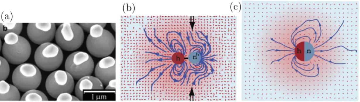
The dimer type of construction is of considerable interest, as it has an increased inherent complexity in comparison to the Janus particle due to the additional degrees of freedom in construction. Its collective dynamics will be determined by a complex interplay of phoretic effects, steric interactions, hydrodynamics and thermal fluctuations. The temperature field around a hot particle obeys the Fourier law, decaying with distance like 1/r. For the phoretic effect, that is proportional to the gradient of the field, implying a decay proportional to 1/r². It has been shown in simulation studies that the hydrodynamic flow field of Janus particles decays like 1/r³, such that for these particles hydrodynamic effects are likely less important than phoretic effects [25]. In case of the dimer however, hydrodynamic interactions decay with 1/r², i.e. the same as the phoretic effect, such that interesting combined effects may result in the dynamics of swimmer ensembles. The experimental realization of chemical dimers and the simulated flow fields of a thermophoretic dimer and a thermophilic Janus swimmer are shown in fig. 1.4.

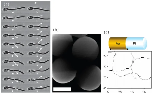
(a) (b) (c)

Figure 1.4: Examples of dimeric microswimmers. a) Experimental realization of a chemically driven dimeric colloidal swimmer. From [19]. b) Simulated flow field of a thermophilic dimer swimmer. c)Simulated flow field of a thermophobic Janus swimmer. Both simulated flow fields are taken from [25].

After this general introduction to the subject matter, the following sections will

(24)

1 Introduction

discuss prerequisites of specific importance to this work in more detail.

1.1 Hydrodynamics

The motion of an incompressible Newtonian fluid is governed by the Navier-Stokes equation

ρ(

∂v

∂t + (v⋅ ∇)v) = −∇p+µ_d∇²v+f (1.1) with the incompressibility condition

∇ ⋅v =0. (1.2)

The velocity field v, the pressure field p and the external forces f all depend on position r and timet. The fluid’s dynamic viscosity is denotedµ_d and its density ρ. An adimensionalization of the Navier-Stokes equation is possible by choosing a characteristic length scale l_c, and a characteristic velocity v_c. For flow past a sphere for example, l_c might correspond to the spheres radius or diameter, while v_c could correspond to the fluid velocity at infinity [26]. This choice then leads to a characteristic timescale t_c = l_c/v_c. The variables in the Navier-Stokes equation can then be rescaled. Choosing v^′=v/v_c, t^′ =t/t_c, p^′=t_cp/µ_d, f^′=l_c²/(µ_dv_c)f and

∇^′=l_c∇, one obtains ρv_cl_c

µ_d (

∂v^′

∂t^′ + (v^′⋅ ∇^′)v^′) = −∇^′p^′+ ∇^′2v^′+f^′ (1.3) for the Navier-Stokes equation. The incompressibility condition reads the same in non-dimensional form, i.e. ∇^′⋅v^′ = 0. The prefactor in eq. (1.3) is the Reynolds number

Re= ρv_cl_c

µ_d . (1.4)

For low Reynolds numbers Re ≪ 1, which is characteristic for many soft matter systems, especially microswimmers, this allows neglecting the l.h.s. of eq. (1.3).

Then, the fluid dynamics are described by the Stokes equation

∇p−µ_d∇²v =f (1.5)

with the same incompressibility condition ∇ ⋅v = 0. Interestingly, in the Stokes equation, the variables are no longer dependent on time. Solutions of the Stokes equation depend on the chosen boundary conditions. A discussion for phoretic processes at colloidal surfaces will be given in chapter 3.

6

(25)

1.2 Colloidal Dynamics

The term colloid is commonly used to describe particles with dimensions in the range of roughly 1 nm up to 10 µm, though these limits are not sharp [27]. The lower limit is set by the requirement that the particle should be larger than the surrounding solvent molecules, whereas the upper limit stems from the idea that colloids should be measurably influenced by Brownian motion. Even for the small- est colloid, the difference in length scales with respect to the solvent (ca. one order of magnitude) is large enough that it should be possible to capture the solvent’s influence on the colloid by a continuum description. For this to be feasible, the typical time scales of solvent and colloid should also be well separated. Experi- mentally measured solvent relaxation times are of the order 10⁻¹⁴ s, whereas the relevant time scales for colloidal motion start at ca. 10⁻⁹ s [27], ensuring a large enough separation to account for solvent effects in an averaged way. A (spherical) colloidal particle of mass M immersed in a fluid will then, due to the separation in time and length scales, experience the averaged interaction with the fluid in two ways. For one, it will feel a random force ξ(t), accounting for the random "kicks"

it gets through thermal fluctuations of the fluid. Then, it will experience a friction force opposite to its direction of movement and proportional to its velocityv, with friction coefficient ζ. Together, the resulting equation of motion for the colloid’s position r reads as

¨

r= −ζv+ξ+ F

M (1.6)

This is the so-called Langevin equation. F describes an external force, but in the following discussion it is assumed that none is present. Since the random force should model thermal noise of the solvent, which has no preferred direction, its average should be zero. Due to the large separation in length and time scales between solvent and colloid, the noise is assumed to be Gaussian white noise, which is delta correlated in time, such that

⟨ξ(t)⟩ =0 (1.7)

⟨ξ(t)ξ(t^′)⟩ =Gδ(t−t^′) (1.8) whereGdescribes the fluctuation strength, which can be shown, using the equipar- tition theorem, to be given by

G=2kBT ζI (1.9)

with I being the identity matrix. Equation (1.6) and eq. (1.8) then determine the motion of a colloidal particle in random solvent and several characteristic properties may be derived from these equations. The Mean Squared Displacement (MSD) is

(26)

1 Introduction

given for small times by

⟨∣r(t) −r(0)∣²⟩ =v(0)v(0)t² (1.10) and for longer times by

⟨∣r(t) −r(0)∣²⟩ =I2kBT

ζ t=I2Dt (1.11)

whereDis the diffusion coefficient. Such a relation between a diffusion and friction coefficient, D=kBT/ζ, is called the Einstein relation.

In the overdamped limit, it is assumed that inertial effects do not play a role, therefore the acceleration term drops out of eq. (1.6). The resulting equation of motion is then given by

v= ξ

ζ . (1.12)

This implies that the vanishing of the average velocity is fully determined by the system temperature and realization of the noise. Since most of the systems investigated in this thesis happen to be in the low Reynolds number regime, this is also a reasonable approximation in the description of these.

1.2.1 Active Colloids

For a Brownian colloid at low Reynolds number, the average velocity is zero according to eq. (1.12). However, a driving force F may act on it, leading to its persistent propulsion. If such driving force is locally produced by the colloid itself, as op- posed to an external field like gravity, the colloid is referred to as self-propelled.

For self-propelled colloids, the propulsion will typically have an inherent direction- ality. Therefore, also the orientation of the colloid, along which the self-propulsion force acts, has to be considered in its description. For the reference case of an active Brownian sphere with fixed propulsion velocity v₀ along its orientation vector e, the Langevin equations describing position and orientation are given by [9]

v=v₀e+

√2Dξ (1.13)

˙ e=

√2D_rξ_r×e (1.14)

with D_r the rotational diffusion coefficient and ξ_r the orientational noise, which is also taken to be Gaussian white noise. The orientational autocorrelation of such a particle decays with

⟨e(t) ⋅e(0)⟩ =exp[

−t

τ_r] (1.15)

8

(27)

1.3 Thermophoresis where τ_r describes a characteristic persistence time. For active Brownian spheres, the MSD also takes on a modified form due to the self-propulsion, given by

⟨∣r(t) −r(0)∣²⟩ =2dDt−2v_o²τ_r²t−2v₀²τ_r²(1−e^−t/τ^r) (1.16) with d the dimensionality. For small times t≪τr this takes the form

⟨∣r(t) −r(0)∣²⟩ =v₀²t²+2dDt . (1.17) The rotational diffusion coefficient D_r can be obtained through the rotational mean squared displacement, which is given by [27]

⟨∣e(t) −e(0)∣²⟩ =2(1−exp[−2D_rt]) (1.18) which for small times 2D_rt≪1 can be approximated by

⟨∣e(t) −e(0)∣²⟩ =4D_rt . (1.19)

1.3 Thermophoresis

Thermophoresis in general describes the effect of an applied temperature gradient on the particle motion of a suspension [28]. Its analogue at the molecular level is thermal diffusion, also called the Ludwig-Soret effect, that refers to the partial segregation of the compounds of a liquid mixture upon application of a temperature gradient. It is a non-equilibrium effect, involving a constant flux of mass in response to the temperature gradient. A colloid immersed in a fluid with a temperature gradient will experience a force due the non-uniform distribution of temperature in the surrounding medium, which leads to a non-vanishing average drift velocity.

Non-uniform distributions of temperature may also induce further non-uniformities, for example in the fluid density distribution, which may also affect force the colloid experiences.

1.3.1 Theoretical Description

Van Kampen obtained a general description for the diffusion of a Brownian particle in an inhomogeneous environment [29], which can be connected to thermophoresis of dilute colloidal suspensions [30] leading to an expression for the colloidal drift velocity v_d. The diffusion equation for the probability density P(r, t)of a particle in a homogeneous medium, including an external potential W(r) that acts on it, is given by

∂P

∂t = ∇ ⋅ [(µ∇W)P +D∇P] (1.20)

(28)

1 Introduction

where µ is the mobility and the diffusion coefficient D is given by the Einstein relation D=µT. In the scenario of an inhomogeneous medium considered by van Kampen, µ, D and T can depend on the spatial coordinate r. Then, a possible generalization reads as

∂P

∂t = ∇ ⋅ [(µ∇W)P + ∇DP] (1.21)

which is the same as

∂P

∂t = ∇ ⋅ [(µ∇W + ∇D)P +D∇P]. (1.22)

Here, the inhomogeneities lead to an additional term ∇DP, referred to as "extra drift". Van Kampen did propose a generalized framework based on consideration of three cases for which the diffusion equation is derived specifically. One of these cases is the diffusion of a Brownian particle in an inhomogeneous surrounding.

This can be applied as a model for a colloid situated in a temperature gradient.

The Kramers’ equation for a Brownian particle describes its dynamics through the evolution of the joint probability of position and velocity g(x, v, t)by

∂g

∂t = −v∂g

∂x +W^′(x)∂g

∂v+ζ(

∂

∂vvg+T∂²g

∂v²) (1.23)

where W^′ = −f denotes the derivative of the potential, i.e. the force f. For high values of ζ, the last term is dominant. Then, one may expand the equation in powers of ζ⁻¹ in the spirit of the Chapman-Enskog procedure [31]. To lowest non- vanishing order, with µ(x) =1/ζ(x)and D(x) =T(x)/ζ(x), the resulting equation is given by

∂P

∂t =

∂

∂x[µW^′P +µ ∂

∂xT P]. (1.24)

This can be reformulated in terms of a continuity equation with flux J as in [29]

∂P(r, t)

∂t = −∇J(r, t). (1.25)

The flux would then be given by [30]

J(r) =nρµ(r)f−µ(r)∇[nρ(r)kBT(r)] (1.26) wherein the notation has been switched from P to particle number density n_ρ and potential V to force f = −V^′. Assuming validity of local equilibrium and the Einstein relation to hold, one may add and subtract kBT(r)∇µ(r)to arrive at [30]

J(r) =n_ρ(r)v_d− ∇[n(r)D(r)] (1.27)

10

(29)

1.3 Thermophoresis

where the drift velocity of the particle is given by

v_d=µf +kBT∇µ. (1.28)

For a more detailed discussion on interpretation of the involved terms and assump- tions see [29] and [30]. Equation (1.27) relates the drift velocity of a particle to its inhomogeneous surrounding given by a spatially inhomogeneous density and value of the diffusion coefficient and/or mobility.

It is interesting to make the connection to the phenomenological expression of thermophoresis. To do so, the phenomenological expression for the mass flux is required. In the framework of non-equilibrium thermodynamics, the entropy pro- ductionς in a binary system showing a diffusive mass fluxJ_k and heat flux J_q can be written as [32, 33]

ς = − 1

T²J_q⋅ ∇T − 1 T

2

∑

k=1

J_k⋅ ∇_Tµ_k. (1.29)

Here, ∇T is the thermal gradient, ∇_Tµ_k is the chemical potential gradient of component k at constant temperature and J_k the mass flux for component k. The phenomenological equations describing thermophoresis in a binary mixture follow from this as [32]

J_q= −L_qq∇T

T² −L_q1∇_T(µ₁−µ₂) (1.30) J₁ = −L_1q∇T

T² −L₁₁∇_T(µ₁−µ₂)

T (1.31)

where Lαβ are phenomenological coefficients fulfilling Onsager reciprocal relations.

A complete derivation can be found in [33]. Taking the solute as species 1, express- ing the mass flux in terms of the solute mole fraction x=n_ρ,1/n˜_ρ and the number densities of the two species as nρ,1 andnρ,2 with ˜nρ=nρ,1+nρ,2, the mass flux reads as [28, 30]

J₁ = −n˜_ρD_m∇x−n˜_ρx(1−x)D_T∇T . (1.32) HereD_T is the thermal diffusion coefficient andD_mthe mutual diffusion coefficient.

These are related to the phenomenological coefficients by [33, 34]

D_m=L₁₁∇_T(µ₁−µ₂)

˜

n_ρT∇x =

L₁₁

˜

n_ρ(1−x)T

∂µ₁

∂x (1.33)

D_T = 1

˜

n_ρT²x(1−x)L_1q. (1.34)

(30)

1 Introduction

In the steady state, the mass flux will vanish: J₁ =0. From this, one obtains S_T =

D_T

D_m = − 1 n_ρ,1n_ρ,2

∇n_ρ,1

∇T = − 1

x(1−x)

∇x

∇T (1.35)

as the ratio of thermal diffusion and mutual diffusion coefficient, which is called the Soret coefficient S_T. The Soret coefficient may take on both positive and negative signs, where a positive value of S_T refers to the more commonly observed thermophobic behavior, while a negative sign indicates thermophilic behavior.

In the case when the solute density n_ρ,1 is low compared to the solvent density n_ρ,2, the mutual diffusion coefficient D_m is equal to the solute diffusion coefficient D and the mass flux of eq. (1.32) may be compared to eq. (1.27), obtaining [30]

vd= ∇D−DβT∇T −DT∇T (1.36) with the thermal expansion coefficient β_T = −(1/n_ρ,2)∂n_ρ,2/∂T.

More commonly used is the expression

vT = −DT∇T (1.37)

to express the thermophoretic velocity. This is only equal to the derived drift velocity if the thermal diffusion coefficient is the dominant term in eq. (1.36), such that ∣D_T∣ >> ∣dD/dT −Dβ_T∣. The validity of this approximation for colloids in complex fluids has been confirmed in simulation studies on thermal diffusion [35].

Instead of the colloid’s velocity, the force acting on it through the temperature gradient may also be used to describe thermophoresis. This thermophoretic force is also linearly related to the temperature gradient through [24]

f_T = −α_T∇kBT , (1.38)

where α_T is the thermal diffusion factor.

The characteristic values used to describe colloidal thermophoresis are the Soret coefficient S_T or the related thermal diffusion factor, which is related to the Soret coefficient by [24]

α_T =T S_T. (1.39)

The Soret coefficient or thermal diffusion factor provides the linear proportionality constant relating the gradients to the response of the colloid.

1.3.2 Experimental and Simulation Results

The thermal diffusion factorα_T is a quantity conveniently used in the description of simulation results, as the forces and temperature gradients are known and directly accessible. More commonly used in experiments to characterize the behavior of colloids is the Soret coefficientS_T of eq. (1.35). As pointed out in the introduction,

12

(31)

1.3 Thermophoresis

S_T depends on a multitude of factors. Notably, it has a complex dependence on temperature and particle size. Experimental results on both temperature and size dependence are shown in fig. 1.5.

(a) (b)

Figure 1.5: Experimental results on the Soret coefficient. a) Temperature dependence of the Soret coefficient for polystyrene particles in a dilute aqueous solution. Taken from [36]. b) Experimental results on the particle size dependence of the Soret coefficient. Taken from [28]. Experimental data for polystyrene beads from [37] (filled squares), [36] (filled circles), [38] (open circles). Data for water-in- oil microemulsions from [39] (open squares).

Braibanti et al. measured the temperature dependence of the Soret coefficient experimentally [36], obtaining good agreement with the following empirical relation

ST(T) =S_T^∞(1−exp[T^∗−T

T₀ ]). (1.40)

This expression relies on three material-dependent, adjustable parameters T^∗, T₀, and S_T^∞. Its functional form describes a particular type of behavior. In the typical case, for low temperatures,S_T is predicted to have a negative sign. Then, the value ofS_Twill increase with rising temperature as a function of the ratioT/T₀, eventually becoming positive afterT^∗. T₀ is a kind of material constant, describing how strong this temperature dependence is. Finally, the Soret coefficient is expected to reach a saturation value ofS_T^∞ for high temperatures. The coefficientS_T^∞ may take on both signs. In most cases, it is positive, as in all examples shown in fig. 1.5a, which also corresponds to an always positive slope. But there are systems in which it takes on negative values, which implies that the switching at T^∗ is from thermophobic to thermophilic behavior instead and the slope is negative throughout [40].

The Soret coefficient of a specific colloid also depends on the particle radius.

Two types of dependence have been found, a quadratic and a linear one. It is so

(32)

1 Introduction

far unclear where this deviation stems from [41].

It is worthwhile to mention here that many colloids carry charges, and that electrostatics have shown to significantly influence colloidal thermophoresis [42].

Still, this thesis will deal with electrically neutral colloids and solvents as a simpler model system of reduced complexity.

14

(33)

2 Simulation Methods

To describe systems of colloidal microswimmers driven by thermophoresis in computer simulations, the complex interplay of swimmer geometry, hydrodynamics, phoresis, molecular-level interactions, and thermal fluctuations has to be accounted for. The dynamics of colloidal systems take place on mesoscopic time and length scales. Atomistic Molecular Dynamics (MD) is suitable mostly for processes on the nanoscale, both in time and space. A full atomistic description of colloidal systems is computationally therefore very expensive and outside the reach of this method.

To circumvent these limitations, coarse-grained methods have been developed, aim- ing at averaging out fast degrees of freedom while maintaining a description of physical interactions precise enough to study mesoscale problems. For colloidal systems, both hydrodynamics and thermal fluctuations are of considerable relevance and a suitable simulation method needs to account for both of these. Simulation studies in this thesis will use Multi-Particle Collision Dynamics (MPC) [43], a mesoscopic simulation method naturally including both hydrodynamic and thermal effects. In MPC, the fluid is described as a collection of point-like particles that only interact through coarse-grained collisions, which due to its efficiency enables simulation on the necessary time and length scales while still describing correct hydrodynamic interactions [44]. MPC includes thermal fluctuations and heat transport by construction, such that in order to study phoretic effects for colloids in a fluid described by MPC, only a suitable way of thermostatting is necessary. The resulting temperature fields, hydrodynamic flow fields and thereby phoretic effects are not imposed but develop naturally, such that one expects to obtain a precise and complete description of phoretically driven swimmers and their mutual interactions, especially as compared to methods in which driving forces are imposed. This chapter will introduce the prerequisites necessary to perform such computer simulation studies on thermophoretic microswimmers.

2.1 Molecular Dynamics

MD simulations are intended to provide a description of the time-resolved properties of many-particle systems. In MD, it is assumed that the many-particle system under consideration obeys the laws of classical mechanics and the corresponding equations of motion are solved numerically to obtain the system dynamics. Each particle i with mass m_i in the system is defined by its position r_i and velocity v_i. Then,

(34)

2 Simulation Methods

Newton’s equation of motion reads as

m_ir¨_i=f_i (2.1)

with the force given as the derivative of the potential energy E

fi= −∇_r_iE . (2.2)

The potential energy E is given by the sum of position-dependent individual contributions of the particles in the system as [45]

E= ∑

i

u₁(r_i) + ∑

i

∑

j>i

u₂(r_i,r_j) + ∑

i

∑

j>i

∑

k>j>i

u₃(r_i,r_j,r_k) +... (2.3) where u₁ accounts for the effect of an external field and the other terms for two- body- (u₂), three-body- (u₃), and eventually also higher order interactions. The most important contributions stem from the external fields and the pair-wise interactions u₂, and in many situations it is sufficient to only consider those. When the pair-wise interaction is modeled by some empiric potential adapted to repro- duce reference values, it may be regarded as an effective potential that implicitly accounts for higher-order interactions. The choice of a suitable pair-wise interaction potential is a crucial step in performing MD simulations. With one at hand, the equations of motion are then solved numerically. In principle, any numeri- cal method to solve differential equations can be used to this aim. The so-called

"velocity-Verlet" algorithm has shown to be an efficient method, suitable both in performance and precision for MD, and it is the one also used in this work. With this algorithm, positions and velocities are updated according to

r_i(t+δt) =r_i(t) +δtv_i(t) + 1 2mi

δt²f_i(t) (2.4)

v_i(t+δt) =v_i(t) + 1

2m_iδt[f_i(t) +f_i(t+δt)]. (2.5) Besides accuracy and performance, a relevant criterion for the choice of integration algorithm is energy conservation. Though many higher-order algorithms show much better short-time energy conservation, their long-term drifts are in fact higher than those of the simpler Verlet-type algorithms, which feature only moderate short-time energy conservation but not much long-term drift [46].

2.2 Interaction Potentials

Suspended colloids interact both with each other as well as with the solvent particles [27]. Experimentally, colloid and solvent interact through interaction potentials on the molecular level. These may be, depending on the precise type of atoms or molecules, repulsive (poor solvent) or attractive (good solvent). Always present in

16

(35)

2.2 Interaction Potentials colloid-colloid interactions is a repulsive hard core type of interaction, which describes that the centers of two colloids can not overlap. For deformable colloids, this repulsion might be softer. Another type of repulsion in between colloids oc- curs when they carry surface charges, these are though frequently screened by the solvent, such that this colloid-colloid interaction is short-ranged repulsive as well.

There can also be attractive interactions in between colloids, for example due to coating with polymer brushes in a poor solvent, which makes their overlap favor- able and induces a short-ranged attraction. Another way to induce short-range attraction in between colloids is through addition of smaller particles, like short polymers. This will induce a so-called depletion interaction.

Atomistic simulations aim at a very precise and complete reproduction of the physical properties of particular substances at specific conditions, and their predic- tive capability hinges on the quality of the interaction potentials. In contrast, in a mesoscopic simulation scenario, the precise choice of colloid-colloid and colloid-fluid interaction does not aim to have a unique mapping to physical quantities. It merely has to capture the essential physics of a colloidal system, such that there is a certain degree of freedom in its choice. The main requirement it has to fulfill always is that it needs to capture a repulsive core, while the details of surface interactions will depend on the system of interest.

In this work, colloid-colloid interactions are modeled as steeply repulsive interactions. One might use hard-sphere interactions to achieve this, however, it is in a molecular dynamics context more desirable to use a steeply repulsive hard-sphere like potential that can still be numerically integrated. The main requirement of colloid-solvent interactions is to have a repulsive core as well. They are chosen likewise, though not only as purely repulsive but also including short-ranged attraction. In every case, a Lennard-Jones (LJ) type of potential is used. The most commonly used LJ potential reads

ULJ,standard(r) =4ε((

σ r)

12

− ( σ r)

6

) +C, r<r_c (2.6) where r is the pairwise distance,ε describes the strength of the interaction, σ the range,r_cis a cutoff beyond which the interaction is zero andCis a shift. The cutoff r_ccould in principle be∞, but is chosen such that the relevant part of the interaction is maintained while saving computational effort by not calculating the potential in between far-away particles, where their mutual interaction is vanishing. A typical value for the cutoff eq. (2.6) is r_c=2.5σ. Choosing r_c=2^1/6σ, the attractive part of eq. (2.6) is cut off and one obtains a purely repulsive interaction potential, referred to as the Weeks-Chandler-Andersen (WCA) potential. C is usually chosen such that the potential is zero at r_c to avoid discontinuities in the calculated energies when two particles approach each other from beyond r_c. This is done for every potential interaction used in this work and will from here on not be mentioned explicitly.

To obtain more flexibility in the interactions, one can also tune the exponents in

(36)

2 Simulation Methods

eq. (2.6) and introduce displacements ∆, arriving at

U(r) =

⎧⎪

⎪⎪

⎪

⎨

⎪⎪

⎩

∞, r≤∆

4ε[( ^σ

r−∆)

2n

− ( ^σ

r−∆)

n

] +C ∆<r<r_c

0, r_c≤r

(2.7)

where the exponentn now allows to tune softness and steepness, while∆allows to enlarge the pairwise distance without modifying the form of the potential. Purely repulsive interactions (WCA) are now obtained with r_c =2^1/nσ+∆. When using displacements∆>0, the effective diameter of a particle iss=σ+∆and a parameter set is given as (s, ∆, ε, n,r/a) where in the last entry "r" indicates a cutoff leading to a purely repulsive interaction while "a" indicates a choice of cutoff giving the full potential including the attractive part. In the latter case it is cut at the value where the energy equals that of eq. (2.6) with ε=1 at r=2.5σ. The precise value of r_c in this case is given by

r_c=∆+ ( 1 2ε(ε−

√

ε(ε+U_LJ,ε=1(2.5σ))))

−¹

n

σ , (2.8)

which is used in this work for every interaction including the attractive part and will not be explicitly mentioned from this point on. The subsets "cf" will be used to denote colloid-fluid interactions, while "cc" will denote colloid-colloid interactions.

2.3 Mesoscale Simulation Techniques

There are several approaches to describe colloidal mesoscale dynamics in computer simulations. Langevin Dynamics (LD) solve the Langevin equation numerically. A distinction is made to Brownian Dynamics (BD), which also solve the Langevin equation, but in the inertia-free limit [47]. LD and BD are in a sense very similar to classic MD simulations, but including a noise and a friction force. For that reason, LD is also used as a thermostat in MD simulations [48]. Since the solvent is treated implicitly, hydrodynamics do not emerge naturally, but may be included through additional forces based on, for example, the Oseen or Rotne-Prager tensor.

When hydrodynamic interactions are included, the method is termed Stokesian Dynamics [49].

Instead of the continuum description of the fluid used in these methods, another approach to treat the problem of the large separation in length and time scales between solvent and solute is to consider the solvent not as atomistically resolved, but to treat larger groups or clusters of fluids as units which move on comparable scales as the solute. These coarsened chunks of fluid are then called "dissipative" particles, and their motion is resolved with the method of dissipative particle dynamics (DPD) [50].

Another approach to resolve mesoscale dynamics of polymers or colloidal suspensions is to employ lattice-based methods. Among these, Lattice Boltzmann (LB)

18

(37)

2.4 Multi-Particle Collision Dynamics methods are prominently used. These work by solving the Boltzmann equation on a lattice, employing specific models to treat the collision terms [50].

Multi-Particle Collision Dynamics (MPC) [43], which has also been called stochas- tic rotation dynamics (SRD) [51] and real-coded lattice gas [52], employs an off- lattice description of coarsened fluid particles which interact through effective collision rules. It has the advantage of including thermal fluctuations by construction in its simplest formulation already, which are crucial in the description of colloidal systems. Due to the method conserving energy locally, thermophoretic effects emerge naturally from it. These features make it a suitable method to describe the fluid in the systems treated in this work.

2.4 Multi-Particle Collision Dynamics

MPC was developed in 1999 by Malevanets and Kapral [43]. The method describes a fluid as a collection of point particles i defined by their positions ri, velocities vi

and mass m_i that do not interact with each other through direct potentials. Fluid particle interactions are instead accounted for in a statistical fashion by coarsening them into multi-particle collisions. At its core, the algorithm consists of two steps, which are illustrated in fig. 2.1. In the streaming step, all particles propagate

(a) (b)

Figure 2.1: Schematics showing the MPC algorithm. In the streaming step a), all particles propagate ballistically. Then, in the collision step b), they are sorted into bins in which multi-particle collisions are performed.

according to their instantaneous velocity for a time h, called the collision time, according to

r_i(t+h) =r_i(t) +hv_i(t). (2.9) Then, collisions takes place. To perform these, the particles are sorted into bins Ψ of a regular grid of side length a. For each bin, the bin-wise center-of-mass velocity