Towards the Contact and Impact Modeling in Finite Element Simulations of High Speed Forming

Towards the Contact and Impact Modeling in Finite El- ement Simulations of High Speed Forming ^*

M. Schwarze

, C. Rickelt

, S. Reese

1Institute of Solid Mechanics, TU Braunschweig, Germany

Abstract

In finite element simulations of high speed sheet metal forming processes the contact between workpiece and forming tools has to be modeled very carefully. Several important aspects have to be taken into account. Robust and locking-free finite element formulations are required to model the sheet forming process, the die has to be considered as a deformable component, and the description of the contact constraints between workpiece and forming tools is a sig- nificant source of shortcomings in modeling. The contact and impact simulation makes high demands on the robustness of finite element formulations. For this reason finite elements with low order ansatz functions are preferred. Furthermore, they prove to be advantageous when automatic meshing tools are applied. To overcome the undesired effects of locking we work with an improved version of the innovative solid-shell concept proposed by [11]. It is based on the concept of reduced integration with hourglass stabilization. The use of this solid-shell finite element allows us to test the influence of the modeling of the die and the contact constraints in a very efficient way.

An overview of so-called macro and micro deformations of forming tools in sheet metal forming simulations can be found in [8]. We show that the deformation of the die has a no- ticeable influence in electromagnetic sheet metal forming. However, in most commercial finite element codes taking into account elastically deformable forming tools requires a full finite el- ement discretization of the die which leads to very high computational effort. Therefore users often assume the tools as being rigid and apply node-based spring-dashpot systems to im- prove the modeling of the interaction between sheet metal and die. But also in this case local interactions cannot be taken into account realistically. As a possible remedy we investigate a fully elastic description of the forming tools in combination with model reduction techniques.

These significantly reduce the number of degrees-of-freedom in the finite element simulation.

For this reason we present different alternatives of this technique.

Keywords:

High speed forming, Solid-shell formulation, Contact modeling, Model reduction techniques

*This work is based on the results of the research group FOR 443. The authors wish to thank the German Research Foundation – DFG for its financial support.

1 Introduction

The development of shell theories, which take the three-dimensional geometry correctly into account, has been a topic of recent research in the field of finite element technology. The goal is to modify classical three-dimensional solid elements with only displacement degrees- of-freedom in such a way, that the undesired effects of locking are eliminated and only one element over the sheet thickness is sufficient for a physically correct result. From the viewpoint of industrial users two further aspects play an important role: the element has to be numerically efficient and robust in the case of large mesh distortions and contact computations. That is why many solid-shell formulations are based on the eight-node hexahedral solid element.

In the development of solid-shells the techniques of finite element technology have to be applied to avoid the undesired effect of locking. One important strategy is the method of incom- patible modes. It is the basis of the enhanced assumed strain (EAS) concept, developed by Simo and co-workers [16, 14, 15]. Based on a mixed variational principle additional ”enhanced”

strains are introduced to avoid non-physical constraints caused by the low order ansatz func- tions. In problems under compression numerical instabilities might arise [20]. In solid-shell finite element formulations this concept is often applied to avoid volumetric, thickness and membrane locking [6, 18, 1, 11]. Keeping in mind, that the number of EAS degrees-of-freedom might in- fluence the robustness of the finite element analysis, i.e. increase the danger of hourglass instability, especially in the case of forming simulations with contact, we strive to work with a minimum number of enhanced degrees-of-freedom.

In high speed forming simulations the elasticity of the die influences the numerical re- sults noticeably. To increase numerical efficiency we apply projection-based model reduction.

Here we consider the methods of modal truncation [3, 4], load-dependent Ritz vectors (LDRV) [5, 4, 10], and proper orthogonal decomposition (POD) [2, 7, 17]. The fundamental idea is to substitute the physical model by a set of modes which well approximate the principal dynamical behaviour. This model reduction does not only reduce the size of our linear components but also preserves the sparsity of the linear part of the Schur complement.

2 Treatment of Locking in Hexahedral Finite Elements

In finite element formulations the undesired effect of locking occurs in different forms. An overview of locking in solid-shell elements with linear and quadratic ansatz functions can be found in [6]. Important strategies to cure locking are the reduced integration concept with hour- glass stabilization, the assumed natural strain method, and the EAS concept. To develop a robust solid-shell formulation which allows large time increments in sheet metal forming simu- lations, we seek to reduce the number of EAS degrees-of-freedom to a minimum.

In sheet metal forming the structure is subject to strong bending. During plastification the material shows nearly incompressible behavior. That is why the transverse shear locking, the thickness locking, and the volumetric locking play the main role. In order to develop a robust

finite element formulation with a minimum number of EAS degrees-of-freedom we investigate here in particular thickness and volumetric locking.

2.1 Thickness Locking

Thickness locking is caused by the linear interpolation of the displacements in thickness direc- tion. Let us consider a bending situation with respect to theη-axis. In this case the termH_ξξof the local displacement gradient tensor has to be constant within the shell plane, but linear over the thickness. The same demand is required forH_ζζ. Unfortunately the linear ansatz functions inζ lead to a constant value forH_ζζ and therefore to a non-physical constraint. To avoid thick- ness locking it is necessary to introduce a linear strain interpolation in thickness direction. This will be done by an EAS ansatz forH_ζζ.

2.2 Volumetric Locking

Volumetric locking in finite element formulations with linear ansatz functions occurs, when the material approaches incompressibility. The fulfillment of the incompressibility condition

detF= 1 (1)

is not possible without artificial constraints. To demonstrate this, let us consider the compatible deformation gradient

Fcomp⋆=Hcomp⋆+1 (2)

evaluated at the shell director. The first two columns of the compatible displacement gradient tensor evaluated at the shell director Hcomp⋆ are linear in ζ. The lack of a linear term in ζ in the third column of H_comp⋆ leads to a constrained solution for the incompressibility condition and, consequently, to volumetric locking. So curing the volumetric locking effect means here to ensure the same order of polynoms in Hcomp⋆. One way is to compute the volumetric part of the element stiffness only in the center of the element. So all terms are constant in the considered point. However, in this case we restrict ourselves to material models with a volume- tric-deviatoric split. The second possibility is to enrich the ansatz functions of the appropriate strain terms. This leads to an EAS ansatz with three enhanced degrees-of-freedom at the shell director. However, in this case we introduce artificial strain components atH_ξζ andH_ηζ, which we attempt to avoid in the treatment of transverse shear locking. For this reason we modify the Q1SPs solid-shell element formulation and enrich onlyH_ζζ.

3 Solid-shell Concept

Starting point of the solid-shell formulation is the two-field functional g1(u^h,H^h_enh) =

B^h₀

P(H˜ ^h) : Gradδu^hdV + gext= 0 (3)

g2(u^h,H^h_enh) =

B^h₀

P(H˜ ^h) :δH^h_enhdV = 0 (4)

in which the displacement vectoru^h and the tensor of enhanced strainsH^h_enhare the indepen- dent variables. The term gext includes the virtual work of the external forces. P^h is the first Piola-Kirchhoff stress tensor. The total strainH^h is additively decomposed into the compatible strainH^h_comp := Grad uand the enhanced partH^h_enh, the interpolation of which is chosen ac- cording to the EAS concept [16, 14, 15]. The index h denotes the finite element discretization of the domain. In the following all values are given in Voigt notation. The interpolation of the total strainH^h does not differ from the one chosen for the hexahedral element formulation proposed by [12]:

H^h= B₀+

j¹₀L¹_hg+j²₀L²_hg M_hg

Ue

:=H^h_comp

+j¹₀L_enhWe

H^h_enh

(5)

For a detailed definition of the variables used in this section see [11]. In contrast to classical finite element formulations the Jacobian matrix is always evaluated in the center of the element.L¹_hgandL_enh are linear inξ, ηandζ, whereasL²_hgdepends bi-linearly on the local co-ordinates. The vectorWe = [W1,W2, ...,W9]^Tincludes the enhanced degrees-of-freedom.

Tacitly we assume thatζ is directed along the thickness direction of the reference ele- ment. In this case the normal through the center of the reference element is given by the vector of local co-ordinatesξ_⋆ :={ξ= 0, η= 0, ζ}. We call it shell director. The element with the shell director is depicted in Figure 1. In the following we split the displacement gradient tensor into

Figure 1: Shell director on solid-shell element

H^h=H^h_⋆ + H^h_△ (6)

in which

H^h_⋆:=H^h(ξ_⋆) (7)

is evaluated on the shell director. The two summands of Equation 6 are given by H^h_⋆ =

B0+j¹₀L¹_hg^ζM_hg Ue

:=H^h_comp⋆

+ j¹₀Lˆ^ζ_enhW^ζ_e

:=H^h_enh⋆

(8)

and

H^h_△=

j¹₀L¹_hg^ξη+j²₀L²_hg

M_hgUe

:=H^h_comp△

+ j¹₀Lˆ^ξη_enhW^ξη_e

:=H^h_enh△

(9)

Following our conclusions in the previous section, we modifyH^h_enh⋆by reducing the num- ber of enhanced degrees-of-freedom from three to one. Therefore the enhanced displacement gradient tensor, evaluated at the shell-director, simplifies to

H˜^h_enh⋆=j¹₀L˜^ζ_enhW₉ (10) in which W9 is the only enhanced degree-of-freedom. FurthermoreL^ζ_enh reduces to

L˜^ζ_enh= 0 0 0 0 0 0 0 0 ζ T

(11) and becomes a vector. Consequently, if we work with an implicit time integration scheme, the consistent linearization of the two field variational functional simplifies noticeably. Instead of solving an three-dimensional equation system to update W^ζ_e, we work now with a scalar equation for W9, which leads to a faster and more robust element formulation. The element requires a smaller memory to store the EAS variables.

A good description of the stress state over the thickness is the main point of interest for the development of the solid-shell element. For this reason a Taylor expansion with respect to the shell director is carried out, finally leading to the relation

P^h ≈P^h_⋆+A^h_⋆

Hˆ^h_comp△+H^h_enh△

(12) In this way the non-linear dependence onζis retained in the constitutive qualities, namely the stressP^h_⋆ :=P

H^h_⋆

and the tangentA^h_⋆:=∂P^h_⋆/∂H^h_⋆. Note, that Hˆ^h_comp△=

j¹₀L¹_hg^ξη+j²₀L²_hg^ζ

M_hgU_e (13)

holds. The analysis of the enhanced degrees-of-freedom is performed at the element level.

They are determined separately by the non-linear scalar equation Rw =

ζ=+1 ζ=−1

L˜^ζTj^1T₀ P^h_⋆dζ 4J₀ (14)

for W9at the shell director, and by the linear equation

W^ξη_e =−KwwKwuUe (15)

for W^ξη_e inside the hourglass stabilization. Due to the linearity of the last equation, only the single value W₉ has to be saved as history variable.

4 Simulation of Electromagnetic Forming (EMF) with Contact

In this chapter we examine the influence of the contact parameters and the die modeling on the simulation results in EMF. Therefore we expand the three-dimensional example considered in [13] by a die made of steel. The thickness is 10 mm and the gap between the undeformed sheet metal and the die is 12 mm. The die is clamped at the upper side. In the finite element simulation of the problem we benefit from the proposed solid-shell formulation which allows us

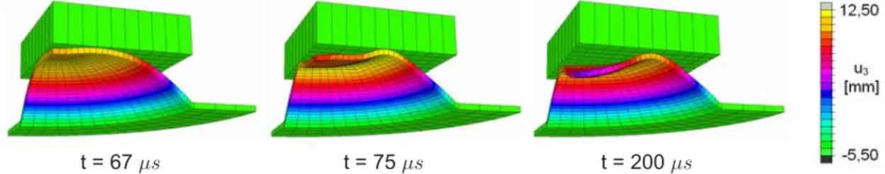
to discretize the sheet metal with only one element over the thickness and 448 elements in the sheet plane. Further we model the contact problem by the use of the three-dimensional version of the classical node-to-segment approach in combination with the penalty method. The elastic material parameters of the die are represented by the Young’s modulus E = 210.000 N/mm² and the Poisson’s ratioν = 0.3. Figure 2 shows the state of deformation before, during, and after the sheet impact. The simulation result of the sheet rebound depends strongly on the

t = 67µs t = 75µs t = 200µs

Figure 2:Impact of the sheet metal at the die

chosen penalty coefficientǫ(Figure 3). By the use of small penalty coefficients the work piece penetrates the die deeply and remains there for few time increments. Due to this fact un- physically high restoring forces are introduced between sheet metal and die which lead to an overestimation of the rebound. However, if we work with an adequate value for the penalty coefficient we are able to simulate a nearly converged solution. This allows us to circumvent the application of the numerically more expensive Langrangian method of contact formulation.

The second point of investigation is the die modeling. For this reason we optionally model the

-8 -6 -4 -2 0 2 4 6 8 10 12 14

0 50 100 150 200 250 300

Displacement [mm]

Time [µs]

ε = 1e3 1e4 1e5 1e6 1e7

Figure 3:Influence of pealty coefficient

-8 -6 -4 -2 0 2 4 6 8 10 12 14

0 50 100 150 200 250 300

Displacement [mm]

Time [µs]

rigid vertically deformable fully deformable

Figure 4: Influence of die modeling

tool as rigid, vertically deformable, and fully deformable structure. Comparing in Figure 4 the converged results of the simulated rebound the dependence of the numerical results on the die modeling becomes obvious. If we assume the tool as being rigid the entire kinetic energy of the sheet metal is reflected at the die and remains in the work piece. An overestimated rebound results. If we the die model as being vertically deformable or fully deformable we analyze a noticeable different result which seems to be more physical. However, this procedure is nu- merically much more expensive and let us consider the application of model reduction on the linearly elastically modeled die.

5 Model Reduction Techniques

In this section we consider model reduction techniques for linear dynamic systems. We start with the ansatz

U=W Q (16)

in whichU is the displacement vector,Qis the vector of the reduced system andWa rectan- gular projection matrix. This approach is inserted into the linear equation of motion

K U+MU¨ =P_ext (17)

in which K denotes the stiffness, M the mass matrix and P_ext the external load vector. This leads to a set of linear equations

W^TK W

K˜

Q+W^TM W

M˜

Q¨ =W^TP_ext

P˜ext

(18)

of reduced order. In the following three different projection-based model reduction methods are summarized. These methods are the modal truncation, the load-dependent Ritz vectors (LDRV) and the proper orthogonal decomposition (POD). They differ in the computation of the projection matrixW.

5.1 Modal Truncation

Modal truncation, also known as modal reduction, is the most simple and popular model re- duction method. The idea is to solve a subset of the generalised eigenproblem in whichWis the reduced modal matrix and Eis the reduced diagonal eigenvalue matrix. After the mass normalization procedure

W^TK W=E, W^TM W=I (19)

the reduced decoupled differential equation system

E Q+IQ¨ = ˜Pext (20)

is obtained.

5.2 Load-dependet Ritz Vectors (LDRV)

The method of load-dependent Ritz vectors is based on the Lanczos algorithm in combiation with a special start vector. Here the static deflection is used as the first Ritz vector so that all following Ritz vectors may be regarded as the balancing of this initial deflection (see [19]).

The advantage of this method is, that no eigenproblem has to be solved. According to [10] the method delivers the reduced coupled differential equation system

TQ¨ +I Q={β1,0,· · · ,0}^Tf(t) (21)

wherein the stiffness matrix and the mass matrix are degenerated to an identity matrixI and a tridiagonal matrix T in generalised coordinates, respectively. If we assume that the load distribution on the structure is constant during the simulation, the projected external load vector P_ext reduces to{β1, 0,· · · ,0}^Tf(t). The scalar valueβ1 =

w^T₁ M w₁ is given by the first not mass normalised Ritz vectorw₁.

5.3 Proper Orthogonal Decomposition (POD)

A third possibility is the POD method. This method is also known as empirical eigenvectors, Karhunen-Lo `eve expansion, principle component analysis, empirical orthogonal eigenvectors, etc. An overview of nomenclatures used in the literature and areas of application are given e.g. in [2]. The mathematical basis for the POD method is the spectral theory of compact, selfadjoint operators which is explained e.g. in the standard text book of [7]. One problem of this ansatz is that even for small systems the eigenvectors of a large spatial covariance matrix have to be calculated. One approach to lower the computational costs is known as the ”method of snapshots”. In this case each POD basis vector

w= m

J=1

βJvˆ_J (22)

is generated out ofmuncorrelated zero-mean snapshots ˆv_J = ˆu_J −u¯ˆ which describe the de- viation from their temporal mean ¯u.ˆ βJ are unknown coefficients which have to be determined.

After some derivations and using the assumption that the investigated process is ergodic (see e.g. [9], [7]) only a reduced eigenproblem of dimensionm

Bβ =λβ B= 1

mVˆ^TVˆ Vˆ = [ ˆv₁,· · · ,vˆ_m] (23) in which ˆVcontains themsnapshots, has to be solved. Finally the empirical eigenvectors w result from

w= ˆVβ. (24)

Consequently the POD vectors are defined as a linear combination of the snapshots.

6 Conclusions

In this paper a new tree-dimensional solid-shell element has been presented to simulate the contact problem of an electromagnetic sheet metal forming process. The element formulation is free of locking and behaves numerically robustly in contact problems. This allows us to work with a strongly decreased number of elements in comparison to a discretization of the sheet metal with the classical Q1 element formulation.

The tree-dimensional contact problem was analyzed by applying the penalty method in the contact formulation. We have shown that a careful choice of the penalty coefficient allows us to circumvent the numerically more expensive Lagrangian method. An further important conclusion is the fact, that the die should be modeled as an elastically deformable structure.

To reduce the numerical effort arising from this point, we present as remedy the techniques of model reduction. The application of these methods in combination with contact problems is a topic of current research.

References

[1] R.J. Alves de Sousa, R.P.R. Cardoso, R.A.F. Valente, R.W. Yoon, J.J. Grcio, and R.M.

Natal Jorge. A new one-point quadtrature enhanced assumed strain (eas) solid-shell el- ement with multiple integration points along thickness - part ii: Nonlinear applications.

International Journal for Numerical Methods in Engineering, 67:160–188, 2006.

[2] R.A. Bialecki, A.J. Kassab, and A. Fic. Proper orthogonal decomposition and modal analy- sis for acceleration of transient fem thermal analysis.Int. J. Numer. Meth. Engng., 62:774–

797, 2005.

[3] A.K. Chopra.Dynamics of structures: Theory and applications to earthquake engineering.

Prentice Hall, 2001.

[4] R.W. Clough and J. Penzien. Dynamics of structures. McGraw-Hill, 1993.

[5] Jianmin Gu, Zheng-Dong Ma, and Gregory M. Hulbert. A new load-dependent Ritz vector method for structural dynamics analyses: quasi-static Ritz vectors. Finite Elements in Analysis and Design, 36:261–278, 2000.

[6] R. Hauptmann, S. Doll, M. Harnau, and K. Schweizerhof. ’solid shell’ elements with linear and quadratic shape functions at large deformations with nearly incompressible materials.

Computer and Structures, 79:1671–1685, 2001.

[7] P. Holmes, John l. Lumley, and Gal Berkooz. Turbulence, coherent structures, dynamical systems and symmetry. Cambridge Monographs on Mechanics, 1996.

[8] R. A. Lingbeek and T. Meinders. Towards efficient modelling of macro and micro tool defor- mations in sheet metal forming. Materials Processing and Design: Modeling, Simulation and Applications, Proceedings of the 9th International Conference on Industrial Forming Processes, pages 723–728, 2007.

[9] M. Meyer and H.G. Matthies. Efficient model reduction in non-linear dynamics using the Karhunen-Lo `eve expansion and dual-weighted-residual methods.Computational Mechan- ics, 31:179–191, 2003.

[10] B. Nour-Omid and R.W. Clough. Dynamic analysis of structures using Lanczos co- ordinates.Earthquake Engineering and Structural Dynamics, 12:565–577, 1984.

[11] S. Reese. A large deformation solid-shell concept based on reduced integration with hour- glass stabilization. International Journal for Numerical Methods in Engineering, 69:1671–

1716, 2007.

[12] S. Reese, P. Wriggers, and B. D. Reddy. A new locking-free brick element technique for large deforamtion problems in elasticity. Computers and structures, 75:291–304, 2000.

[13] M. Schwarze, A. Brosius, S. Reese, and M. Kleiner. Efficient finite element and contact procedures for the simulation of high speed sheet metal forming processes. InProceed- ings of the 2nd International Conference on High Speed Forming, Dortmund, Germany, 2006.

[14] J. C. Simo and F. Armero. Geometrically non-linear enhanced strain mixed methods and the method of incompatible modes. International Journal for Numerical Methods in Engi- neering, 33:1413–1449, 1992.

[15] J. C. Simo, F. Armero, and R. L. Taylor. Improved versions of assumed enhanced strain tri-linear elements for 3d finite deformation problems. Computer Methods in Applied Me- chanics and Engineering, 110:359–386, 1993.

[16] J. C. Simo and M. S. Rifai. A class of mixed assumed strain methods and the method of in- compatible modes. International Journal for Numerical Methods in Engineering, 29:1595–

1638, 1990.

[17] L. Sirovitch. Turbulence and the dynamics of coherent structures part I-III. Quarterly of Applied Mathematics, 45:561–590, 1987.

[18] L. Vu-Quoc and X. G. Tan. Optimal solid shells for non-linear analyses of multilayer com- posites. i. statics. Computer Methods in Applied Mechanics and Engineering, 192:975–

1016, 2003.

[19] E.L. Wilson, M. Yuan, and J.M. Dickens. Dynamic analysis by direct superposition of Ritz vectors. Earthquake Engineering and Structural Dynamics, 10:813–821, 1982.

[20] P. Wriggers and S. Reese. A note on enhanced strain methods for large deformations.

Computer Methods in Applied Mechanics and Engineering, 135:201–209, 1996.